PIO I-II tendencies case study. Part 1. Mathematical modeling



PIO I-II tendencies case study.

Part 1. Mathematical modeling

Adrian TOADER, Ioan URSU



atoader@incas.ro iursu@incas.ro

“Elie Carafoli” National Institute for Aerospace Research

Abstract

In the paper, a study is performed from the perspective of giving a method to reduce the conservatism of the well known PIO (Pilot-Induced Oscillation) criteria in predicting the susceptibility of an aircraft to this very harmful phenomenon. There are three interacting components of a PIO – the pilot, the vehicle, and the trigger (in fact, the hazard). The study, conceived in two parts, aims to underline the importance of human pilot model involved in analysis. In this first part, it is shown, following classical sources, how the LQG theory of control and estimation is used to obtain a complex model of human pilot. The approach is based on the argument, experimentally proved, that the human behaves “optimally” in some sense, subject to his inherent psychophysical limitations. The validation of such model is accomplished based on the experimental model of a VTOL-type aircraft. Then, the procedure of inserting typical saturation nonlinearities in the open loop transfer function is presented. A second part of the paper will illustrate PIO tendencies evaluation by means of a grapho-analytic method.

1. Introduction

From the Wright Flyer to fly-by-wire, the phenomenon of pilot-induced oscillation (PIO) has been observed on almost every aircraft, either prototype, experimental or operational, military or commercial. Thus, PIO remains a permanent challenge for the aircrafts designers. PIO is a phenomenon usually due to adverse aircraft-pilot coupling during some tasks in which “tight closed loop control of the aircraft is required from the pilot, with the aircraft not responding to pilot commands as expected by the pilot himself” [1]. “Tight closed loop control” concerns as a rule takeoff, landing, aerial refueling, and formation flying. PIO supposes to have the pilot in the closed loop, but it should be emphasized that there is no blame placed on the pilot for the resulting oscillation (therefore other designations, such as:

pilot-in-the loop oscillation or aircraft-pilot coupling have been suggested instead ofPIO).

Indeed, PIO is homologated as factual if there is at least one measurable aircraft state that is 180 degrees out of phase with at least one measurable pilot control input [2]. In other words, PIO is triggered as an aircraft motion totally adverse to pilot intentions and efforts (the third interacting component of the PIO is “a trigger” [2], i.e., in fact, the hazard).

PIOs have caused numerous accidents with results ranging from minor damage to total loss of the aircraft and pilot.

Predicting PIO is difficult and becomes even more difficult with the advent of new technologies such as active control and fly-by-wire flight control systems. This has been demonstrated by recent events involving Boeing 767 & 777, YF- 22A, YF-16, JAS-39, X-5, X-15, Shuttle, Falcon 900 and the list can continue [2]. Theoretical studies and flight test methods lead, however, to recommended practices exposing PIO tendencies, if they exist, so that the catastrophic events can be minimized or eliminated.

According to common references (see, for example, [3]), PIOs are categorized depending essentially on the degree of nonlinearity in the event:

• Category PIO I: linear oscillations resulting mainly from excessive input or state time delay

• Category PIO II: quasi-linear oscillations resulting mainly from some nonlinear dynamics such as rate or position saturation.

• Category PIO III: enough evasive defined as completely nonlinear oscillations. This classification is rather theoretical, didactic, physical events being ever more complex and pretty difficult to decipher.

The analysis of the aircraft dynamics with mathematical models of the pilot-in-the-loop, understudied by simulations of these models, make up in helpful tools in predicting PIOs. As a mathematical model of the human pilot, a static gain [1]is often considered.

Attempts to describe the behavior of the human pilot in the loop are given in [4], in frequency domain, and in [5], [6], in the time domain of the optimal control.

This paper is a first part of a study of PIO I-II tendencies using as object of application the longitudinal channel of a hovering VTOL-type aircraft [7], represented by a five-dimensional system. Firstly, in Section 2, a model of the human pilot is deduced as Modified Optimal Control Pilot (MOCM), nearly following [8]. The pilot’s effective time delay is assimilated to a second order linear system by means of a Pade approximation. Then, in Section 3, position and rate saturation blocks are inserted in the closed loop scheme in order to expose Category II PIO tendencies of the aircraft dynamics. Describing function in the case of position saturation is inferred and a general equation susceptible toprovidethe limit cycle as PIO paradigm is presented. In Section 4, the dynamic model of pilot is validated by comparison with an experimental model [8]. A conclusive Section 5 underlines the interest of the proposed method in the prominence of PIOs.

2. Dynamic human pilot model synthesis in terms of optimal control

Starting from the aircraft dynamics written in the well known invariant linear system

,

x Ax  B Ew y Cx D (1)

MOCM [8] (see block diagram given in Fig. 1) substitutes the neuromuscular pilot pure

delay

e

s [4] by a second order dynamics derived from a second order Pade approximation

, ,

d d d d p d d d p : d

x  A x B u u C x u  u (2)

The two dynamics (1), (2) are thus concatenated as an extended plant dynamics

,

s s s s p s s s s p

x A x B u E w y C x D u (3)

where





T

T T

0 0

, d , , , ,

s d s s s s d s

d d

A BC B E

x x x A B E C C DC D D

A B

     

 

_{ }  _{ } _{ } _{ } 

 

     (3′)

In the second step, a control law which minimizes the performance index



T 2 2



E , 0

p y y

J  _ y Q y   r  f Q      r f (4)

will be performed. By defining a new state vector   xT_s uT_p_T, the system (3) is

,

o o p o o o

A B u E w y C v_y

         (5)

where v_yis the observation zero mean Gaussian white noise with intensity V_y 0 and





0

0 0 0

0 0 0 1 0

, , ,

d

o d d o o o d

A BC B E

A A B B E C C DC

     

     

_{ } _{ } _{ } 

     

     

D (5′)

Fig. 1. Conceptual block diagram of the human pilot dynamic model

Optimal control technique LQG is applied and the result is a full state feedback law

1 T 0

* _{ˆ ˆ}

p p

u     g f B K ₍₆₎

where ˆ is the estimate of the  and K is the solution of the Riccati equation

T T

T 1 T

T T

0, s y s s y s

o o o o c o

s y s s y s

C Q C C Q D

A K KA Q KB f Bo K Q

D Q C D Q D r

 _ _

     

 _ 

 

(7)

In the third step of synthesis, the structure of neuro-motor lag block, Fig. 1, is determined



1



1 1 1



1



* _{, , ˆ} *_{, : , , , , : ˆ}

p n s n p n p n c p s

u   g  g x g _u  _ g _ l  _ g  g u  l x ₍₈₎

and one thus obtains

* *

p p c

u u u



    ₍₉₎

A simple way to model the physical limitation of the human pilot is to add a Gaussian noise to the control (this maneuver reduces the solution (6) to a suboptimal control law)

u

v u_c

p p c u

u  u  _ u  _ v _ (9′)

Given the coupled systems (5), (9′)

control noise

y

v

obs

y

c

u

p

u



d

u

optimal estimator

observation noise observation

w

aircraft

neuromotor lag gain

u

v

delay

displays

1 1 c 1 1, 0 1 y

A B u E w y C v

        (10)





1 1 1 1

0 0

0 0 0 0

0 0 1 1 0 1

: , , : , : , :

/ / /

d

d d d

u

A BC B E

w

A A B B E C C DC D w

v                  _{ }  _{ } _{ }  _{ }    _{ }   _   _        1  p p

the fourth step of synthesis consists in deriving of the associated Kalman estimator









T 1 T T 1

1 1 1 1 1 1 1 1 1 1 1 1 1 1 1

1

0

diag , 0 0

ˆ ˆ , ,

: , ,

c y y y

u u

A FC FC B u Fv F C V A A W C V C

W W V W V

 

                  

    



(11)

The resulting system (10) will be extended with the estimator dynamics (11)



0



,



0 1



0 0 0 ˆ 0 0 , 0 0 ˆ ˆ 1 1 1 0 1 1 1 1 1 1 1 1 1 1 d p y y C C l l v w I C C u y v w F E FC l B A FC l B A                                                                                (12)

This is the closed loop system pilot-aircraft; the model of the pilot dynamics simply follows from (11), (9′), (2)





1 1 1 1

1

T

T T T

0 0 0

1 0 0 0 1

0

0 0 0

0 1

/ / / :

ˆ

: : , :

y y

p p p p

u u

d d

d p p p p p d

A FC B l F F

v v

x l x y A x B y E

v v

B A

u C x C x x u x

          _{  }       _     _ _{ } _  _{ }    _ _           _{ } _ _           _{ }   ₍₁₃₎

The step five of the synthesis, represented by the explicit determination of the matrices in (12), (13), supposes an attentive trial and error procedure for the selection of the noise intensities W V₁, _y in order to obtain the signal noise ratios 2 0 003.

i i

u u

V   and

2 0 01.

i i

y y

V   , which correspond to normalized control noise and normalized observation noise of −25 dB and −20 dB [5], [6], [7], respectively. With that end in view, covariance value Pof the state vector in (12), given by the Lyapunov equation

0

T

T _{ }

 _{cl cl cl}

clP PA B QB

A , Qdiag



W₁,V_y



(14)

will be used to calculate the covariance of the vector yT 



y₀ u



T

T T

cl cl cl cl

T

E yy_  _ C PC D QD (14′)

          1 1 1 1 1 1 1 1 FC l B A FC l B A

Acl 

      F E B_cl 0 0 1         0 0 1 C C

C_{cl }

      I D_cl 0 0

0 _(14′′)

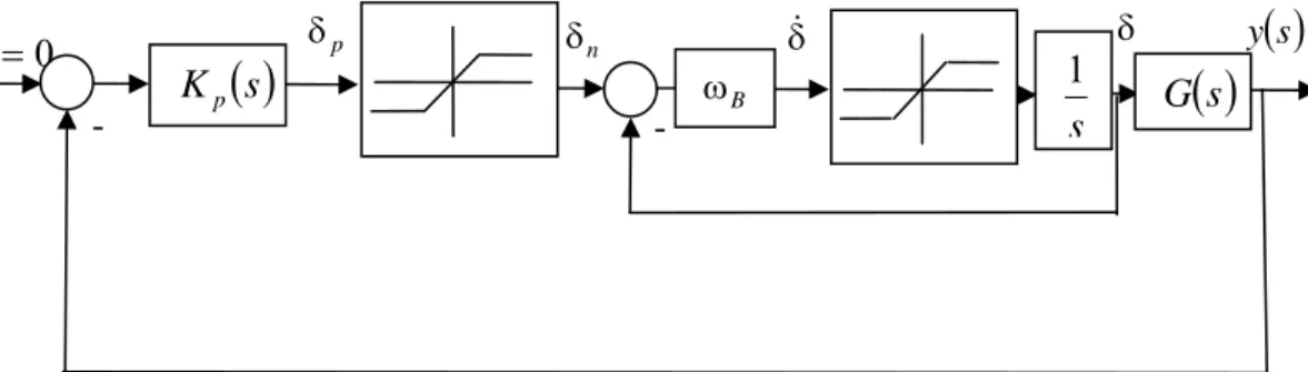
3. Linearization of the saturation type nonlinearities. Describing function method A typical block diagram for the study of Category PIO I-II is shown in Fig. 2. Herein, two basic nonlinearities, usual in flight control, are involved: a position saturation, related to control stick displacement limits (corresponding to flight control surface rotation limits) and a rate saturation, mainly related to flow rate limits of the hydraulic servoactuator). In figure, specifically to the auto-oscillation searching, r0 is the null reference. is the model of pilot (a constant will correspond to the static model),

 

s K_p

p

K _p is the control signal

elaborated by pilot, _n is the control signal to the output of position saturation element,  is the effective control, G

 

s is the model of aircraft, y

 

s is the output. The angular frequency

is in connection with the time constant of the servoactuator.

B 



 y

 

s

p

 _

n 0



r

-

- 

s

K

_p _B

1

_G

 

_s

s

Fig. 2. Block diagram of the system with position and rate saturations

.

0

r _u y

a) general nonlinearity b) position saturation nonlinearity Fig. 3. Schemes for the deduction of the describing function

In order to develop a specific PIO paradigm of limit cycle analysis, the first harmonic

linearization, also called the describing function method, [9] will be applied to the saturation

nonlinearities. This procedure will give the describing function of the nonlinearity, an equivalent gain depending on both amplitude and frequency of the harmonic auto-oscillation (limit cycle), susceptible to propagation in the control loop shown in Fig. 2. The procedure is legitimate if some basic conditions are fulfilled: a) the system is autonomous



r0



; b) at any point in the system there will be a periodic signal; c) L s

 

is a system that is a low pass filter (filter hypothesis).

To specialize, if the input signal to the nonlinear element is a sinusoid

 

sin 2



0



y t a  t , the output surely is not a sinusoid (for a ideal relay, for instance, the -

 

L s

0

r _u y

 

L s

-

output is +A, when input is positive, and –A, when the input is negative; A is some constant). Thus, the output is in fact a square wave. This periodic signal can be described by a Fourier series (the symmetry of the signal above also ensures that only odd harmonics are present)

 



0



1 odd

4 sin 2 ,

k

n n

A

N t n

n



  

t

  





When this wave goes through the linear system, the transfer function L s

 

will selectively filter out the higher frequencies in the Fourier series, and will selectively pass the lower frequencies (in large, only the basic frequency   _{ }).

Let’s define the describing function of a nonlinear element as the complex ratio of the

fundamental component of the nonlinear element by the input sinusoid. To illustrate the

ideas, the case of position saturation is shortly treated. Consider the nonlinearity in Fig. 3b)

 





 

 

 

 

if

sat if

if ,

, ,

L L

L L

L L

P y t P

y t y t P y t P

P y t P

   



_    

    



and the Fourier series development

 





 

 

 





 



 



   



 



  

0

1

2 2 2

0 _{0 0 0}

sat cos sin

2

1 1 1

sat d , sat cos d , sat sin d

n n

n

n n

a

y t a n t b n t

a y t t a y t n t t b y t n t t





  

 

   _    _

           

  













The saturation nonlinearity is an odd function, thus by virtue of the filter hypothesis only the coefficient needs to be calculated. Associating the position saturation value and the corresponding argument

1

b P_L

1

 , one obtains

 

1 1

1 1

sin sin L sin , : L

L

P P

P a

a a

   

     _{ }   

 

therefore the describing function of the nonlinearity sat

 

y is given by the ratio





 

 

 









 

1

1

2

2 1

1 1

0

1 1

1 1

1 1

2 4

4 4 2

; sin sin sin 2 c

2 2

cos sin cos sin

2

sin cos sin :

/ _L

L L

L L L L

P

N a P a d P d

a a a

P P P P

a a a a

N

 



 

 



         

    

  

     

 _   _{   } _{  }

       

      











os 

(15)

In the case of rate saturation, the gain N, having a more complicate structure, depending of

: RL

a  

, RL– rate saturation value, will be used directly in part II of the paper. So far, let’s

collect the linear parts of the system pilot-aircraft, Fig. 2, into the transfer function

.

The nonlinearities are then represented by the describing function

 

s

G

p 



_{ }

p K G s

 

 N

0



r

-



, 0; L, L



N a  P R

K

_p

   

s

G

s



, ; _L, _L



N a  P R

, see Fig. 4. Note that

K

_p

   

s

G

s

is a function only of frequency, while N

0

,

a

is a function of amplitude and frequency. Opening the feedback loop, the stability of the loop transfer functions is assessed by a system of two equations with two unknowns



, 0; L, L

    

p 1

N a  P R K s G s  0 (16)

Fig. 4. Block diagrams showing the insertion of the describing function in the scheme of Fig. 2

4. Validation of the human pilot dynamic model

Let’snow consider the case of human pilot performing the hovering control of a VTOL-type aircraft [101], [11] and [7]. Briefly, the pilot’s task was to minimize longitudinal position errors while hovering in turbulent air. The aircraft model and the displayed outputs for the experiment deployment were

0 095 0 0 0 0 0 1

0 0 0 0

0 1 0 0 0 0 0 :

0 0 0

0 0

0 0 0 1 0

.

g g

u u

h h

u u q

u u

X X g

u u

w Ax B Ew

x x

M M M M

q q 



         

   _       

         

            

         

         

  _    _{ } _  _{ }

     

  

 

(17)

     

 

     

 

 

 



0 1 0 0 0

0 3 0 068 . 0 068 . 0

0 0 0 1 0

81 . 9 0 0 1 . 0 1 . 0

0 0 0 0 095 . 0

A

,

     

 

     

 



0 017 . 0

0 0 0

B

(17′)

0 1 0 0 0

0 0 1 0 0

i.e. 0

0 0 0 1 0

0 0 0 0

, , ,

g

h

h

u u

u x

y Cx D D

x q

q  

     

     

           

     

  _   

   _{  }

  

(18)

where u_g − longitudinal component of the gust velocity [m/s]; u − velocity perturbation

h

stick input [mm]; − speed stability parameter [rad/m-sec]; − pitch rate damping [1/sec]; − control sensitivity [rad/sec2/mm]; − longitudinal drag parameter [1/sec];

u

M M_q



M X_u

g− gravitational constant, 9.81 [m/sec2]; u and q are the first derivatives of x_h, and , respectively.



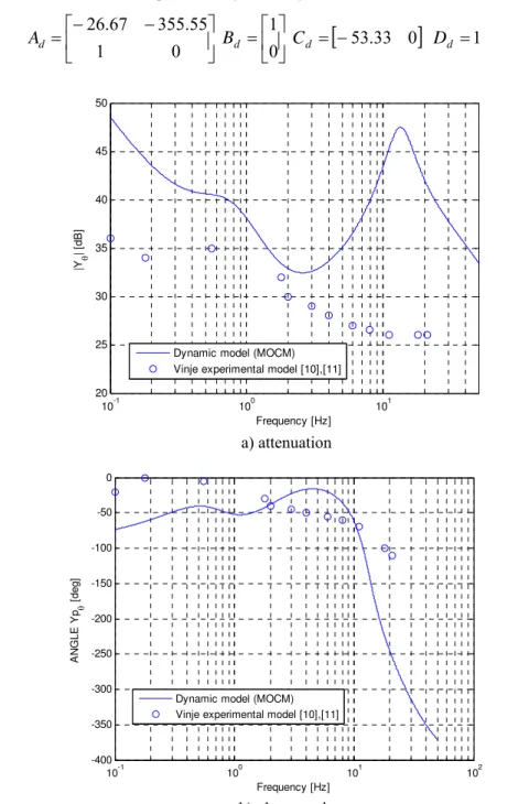
Using a second order Pade approximation of the pilot pure time delay (see Fig. 1), the matrices of the equivalent dynamic system (2) are

s 15

0.

   



 



0 55 . 355 1

67 . 26

d

A _

   d

B _

 

0

1

_

_

0 33 . 53

  d

C D_d 1 (2′)

10-1 50

45

40

35

100 101

20 25 30

Frequency [

|Y 

| [

d

B

]

Dynamic model (MOCM) Vinje experimental model [10],[11]

Hz] a) attenuation

10-1 100 101 102

-400 -350 -300 -250 -200 -150 -100 -50 0

Frequency [Hz]

AN

G

L

E Yp



[d

e

g

]

Dynamic model (MOCM) Vinje experimental model [10],[11]

b) phase angle

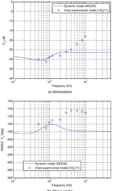
The validation of the dynamic model (13) was performed by a trial and error procedure, having as comparison terms the experimental results given in [10], [11], [7].

10-1 100 101

-40 -35 -30 -25 -20 -15 -10 -5 0

Frequency [Hz]

|Yx

| d

B

Dynamic model (MOCM) Vinje experimental model [10],[11]

a) attenuation

10-1 100 101

-300 -280 -260 -240 -220 -200 -180 -160 -140 -120 -100

Frequency [Hz]

AN

G

L

E

Yx

[d

e

g

]

Dynamic model (MOCM) Vinje experimental model [10],[11]

b) phase angle

Fig. 6. Validation of the pilot dynamic model. Bode diagrams of the transfer function Y_x

A suitable covariance matrix, ensuring the prescribed normalized noises, was found



4 3 3 5



diag 14 46. 6 62 10. 2 53 10. 4 11 10. 1 31 10. 6 1 10.

Q          6 (19)

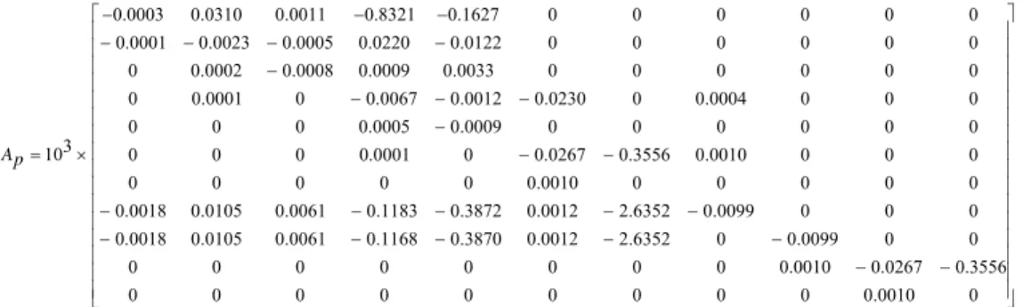
realize a series loop composed by an inner feedback loop and an outer  x_hfeedback loop. Thus, the machinery of dynamic pilot design is testified. The resulting numerical values of the pilot matrices are (see (13))

                                                             0 0 0 0 0 0 0 0 0 0 3556 . 0 0010 . 0 0 0 0 0 0 0 0 0 0 0099 . 0 0 6352 . 2 0012 . 0 3870 . 0 1168 . 0 0061 . 0 0105 . 0 0018 . 0 0 0 0099 . 0 6352 . 2 0012 . 0 3872 . 0 1183 . 0 0061 . 0 0105 . 0 0018 . 0 0 0 0 0 0010 . 0 0 0 0 0 0 0 0 0010 . 0 3556 . 0 0267 . 0 0 0001 . 0 0 0 0 0 0 0 0 0 0009 . 0 0005 . 0 0 0 0 0 0 0004 . 0 0 0230 . 0 0012 . 0 0067 . 0 0 0001 . 0 0 0 0 0 0 0 0033 . 0 0009 . 0 0008 . 0 0002 . 0 0 0 0 0 0 0 0122 . 0 0220 . 0 0005 . 0 0023 . 0 0001 . 0 0 0 0 0 0 1627 . 0 8321 . 0 0011 . 0 0310 . 0 0003 . 0 3 10 p A  0010 . 0 0267 . 0 0 0 0 0 0 0 0 0 0  

These numerical data will serve now to evaluate the robustness of the system with the designed dynamic pilot. The plant-pilot equations (1) and (13) are such resumed

, _{p p p p} , , _{p p p}

xAxBx  A x B y y Cx u C x ₍₂₀₎

and then concatenated

0

δ: δ, 0

0 e e d e e: p

p p p p p p

x A x B x

A B u C x C x

x B C A x

         _               _{ }              x    x    _  (21)

in order to get the transfer u_d, in other words, the open loop transfer function G_ol

 

s

 

_{ }

 





1

: d

ol Ce

Bo

equen

e e

u s

G s sI A B

s



  

 (22)

de Diagram

Fr cy (rad/sec)

10-1 100 101

-630 -540 -450 -360 -270 -180 -90 System: dinami 100 c deg) ec): 0 rad/sec able? Y

Phase Margin ( : 20.1

Delay Margin (s .0946

At frequency ( ): 3.71

Closed Loop St es

P has e ( d eg ) -50 0

50 System: dinamic

Gain Margin (dB): 3.69 At frequency (rad/sec): 6.67 Closed Loop Stable? Yes

M agn itud e ( dB )

The transfer function G_ol

 

s is in fact the product K_p

   

s G s , where

 





1

 





1

,

p p p p

K s C sIA  B G s C sIA  B (23)

but from calculus reasons, the variant (22) is preferable.

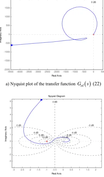
The open loop transfer function G_ol

 

s provides stability margins of the system, in terms of the classical Bode characteristics, see Fig. 7.

The application of the robust stability analysis criterion for PIO prediction [12] leads to the results shown in Fig. 8. The criterion uses the MOCM of the pilot, as defined in Section 2, and is based on the so-called vector stability margin. Accordingly to the criterion, the vector margin is the minimum distance of the open loop pilot-vehicle transfer function from the critical point,  1 j0, in the Nyquist plane.

-4500 -4000 -3500 -3000 -2500 -2000 -1500 -1000 -500 0 500 -2000

-1500 -1000 -500 0 500 1000 1500 2000

0 dB

Nyquist Diagram

Real Axis

Im

agi

nar

y

A

x

is

a) Nyquist plot of the transfer function G_ol

 

s (22)

-3 -2.5 -2 -1.5 -1 -0.5 0 0.5 1 1.5 2 -3

-2 -1 0 1 2 3 4 5

6 0 dB

-10 dB-6 dB -4 dB

-2 dB

10 dB 6 dB 4 dB 2 dB

Nyquist Diagram

Real Axis

Im

agi

nar

y

A

x

is

b) zoom on a)

5. Conclusion

An approach of PIO I-II tendencies is sketched. The first part of the paper proposes a mathematical modeling based on a dynamic model of the pilot. An application is made considering the concrete case of a hovering VTOL-type aircraft. Part two of the paper will illustrate PIO tendencies evaluation by means of a grapho-analytic method.

REFERENCES

[1] F. AMATO, R. IERVOLINO, S. SCALA, L. VERDE, Actuator design for aircraft robustness versus category PIO, Proc. of the 7th Mediterranean Conference on Control and Automation [MED 99] Haifa, Israel, June 28-30, 1999.

[2] D. G. MITCHELL, D. M. KLYDE, Recommended practices for exposing pilot-induced oscillations or tendencies in the development process, USAF Developmental test and Evaluation Summit, November 16-18 2004, Woodland Hills, California, AIAA 2004-6810.

[3] D. M. KLYDE, D. G. MITCHELL, A PIO Case study – Lessons learned through analysis, AIAA Atmosphere Flight Mechanics Conference and Exhibit, August 15-18, 2005, San Francisco, California, AIAA 2005-5813.

[4] R.A.HESSTheory for aircraft handling qualities based upon a structural pilot model, Journal of

Guidance, Control, and Dynamics, 12, 6, 792-797, 1989.

[5] D. L. KLEINMAN, S. BARON, W. H. LEVISON, An optimal control model of human response, Part 1: Theory and validation, Automatica, 6, 3, 357-369, 1970.

[6] S. BARON, D. L. KLEINMAN, W. H. LEVISON, An optimal control model of human Response, Part

II: Prediction of human performance in a complex task. Automatica, 6, 3, 371-383, 1970 [7] D. L. KLEINMAN, S. BARON, Manned vehicle systems analysis by means of modern control theory,

NASA CR-1753, Washington, D.C., June 1971 (DECLASSIFIED).

[8] J. B. DAVISON, D. K. SCHMIDT, Modified optimal control pilot model for computer-aided design

and analysis, NASA-TM-4384, 1992.

[9] H. K. KHALIL, Nonlinear systems, 3rd Edition, Prentice Hall, 2002.

[10] E. W. VINJE, D. P. MILLER, Interpretation of pilot opinion by application of multiloop

models to a VTOL flight simulator task, NASA SP-144, March, 1967.

[11] E. W. VINJE, D. P. MILLER, An analysis of pilot adaptation in a simulated multiloop

VTOL hovering task, NASA SP-192, March, 1968.