Secondary calcification and dissolution respond differently to future ocean conditions

(1)

BGD

11, 12799–12831, 2014

Secondary calcification and

dissolution

N. J. Silbiger and M. J. Donahue

Title Page

Abstract Introduction

Conclusions References

Tables Figures

◭ ◮

Back Close

Full Screen / Esc

Printer-friendly Version Interactive Discussion

Discussion

P

a

per

|

Discus

sion

P

a

per

|

Discussion

P

a

per

|

Discussion

P

a

per

|

Biogeosciences Discuss., 11, 12799–12831, 2014 www.biogeosciences-discuss.net/11/12799/2014/ doi:10.5194/bgd-11-12799-2014

This discussion paper is/has been under review for the journal Biogeosciences (BG). Please refer to the corresponding final paper in BG if available.

Secondary calcification and dissolution

respond di

_ff

erently to future ocean

conditions

N. J. Silbiger and M. J. Donahue

University of Hawai’i at M ¯anoa, Hawai’i Institute of Marine Biology, P.O. Box 1346, K ¯ane’ohe, Hawai’i, 96744, USA

Received: 8 August 2014 – Accepted: 13 August 2014 – Published: 2 September 2014

Correspondence to: N. J. Silbiger (silbiger@hawaii.edu)

(2)

BGD

11, 12799–12831, 2014

dissolution

Title Page

Tables Figures

◭ ◮

Back Close

Full Screen / Esc

Discussion

P

a

per

|

Discus

sion

P

a

per

|

Discussion

P

a

per

|

Discussion

P

a

per

Abstract

Climate change threatens both the accretion and erosion processes that sustain coral reefs. Secondary calcification, bioerosion, and reef dissolution are integral to the struc-tural complexity and long-term persistence of coral reefs, yet these processes have received less research attention than reef accretion by corals. In this study, we use

5

climate scenarios from RCP8.5 to examine the combined effects of rising ocean acidity and SST on both secondary calcification and dissolution rates of a natural coral rub-ble community using a flow-through aquarium system. We found that secondary reef calcification and dissolution responded differently to the combined effect of pCO2and temperature. Calcification had a non-linear response to the combined effect ofpCO₂

-10

temperature: the highest calcification rate occurred slightly above ambient conditions and the lowest calcification rate was in the highest pCO2-temperature condition. In contrast, dissolution increased linearly withpCO₂-temperature. The rubble community switched from net calcification to net dissolution at+272 µatmpCO2and 0.84

◦

C above ambient conditions, suggesting that rubble reefs may shift from net calcification to net

15

dissolution before the end of the century. Our results indicate that dissolution may be more sensitive to climate change than calcification, and that calcification and dissolu-tion have different functional responses to climate stressors, highlighting the need to study the effects of climate stressors on both calcification and dissolution to predict future changes in coral reefs.

20

1 Introduction

In 2013, atmospheric carbon dioxide (CO₂(atm)) reached an unprecedented milestone of 400 ppm (Tans and Keeling, 2013), and this rising CO2(atm)is increasing sea-surface temperature (SST) and ocean acidity (Caldeira and Wickett, 2003; Cubasch et al., 2013; Feely et al., 2004). Global SST has increased by 0.78◦C since pre-industrial

25

(3)

BGD

11, 12799–12831, 2014

dissolution

Title Page

Tables Figures

◭ ◮

Back Close

Full Screen / Esc

Discussion

P

a

per

|

Discus

sion

P

a

per

|

Discussion

P

a

per

|

Discussion

P

a

per

|

the end of this century (Meinshausen et al., 2011; Van Vuuren et al., 2008; Rogelj et al., 2012). The Hawai‘i Ocean Time-series detected a 0.075 decrease in mean annual pH at Station ALOHA over the past 20 yr (Doney et al., 2009) and there have been similar trends at stations around the world including the Bermuda Atlantic Time-series and the European Station for Time-series Observations in the ocean (Drupp et al., 2013).

5

pH is expected to drop by an additional 0.14–0.35 pH units by the end of the 21st century (Bopp et al., 2013). All marine ecosystems are at risk from rising SST and decreasing pH (Doney et al., 2009; Hoegh-Guldberg et al., 2007; Hoegh-Guldberg and Bruno, 2010), but coral reefs are particularly vulnerable to these stressors (reviewed in Hoegh-Guldberg et al., 2007).

10

Corals create the structurally complex calcium carbonate (CaCO₃) foundation of coral reef ecosystems. This structural complexity is at risk from climate-driven shifts from high-complexity, branched coral species to mounding and encrusting growth forms (Fabricius et al., 2011) and from increases in the natural processes of reef destruction, including bioerosion and dissolution (Wisshak et al., 2012, 2013; Tribollet et al., 2006).

15

While substantial research attention has focused on the response of reef-building corals to climate change (reviewed in Hoegh-Guldberg et al., 2007; Fabricius, 2005; Pandolfi et al., 2011), secondary calcification (calcification by non-coral invertebrates and calcareous algae), bioerosion, and reef dissolution that are integral to maintaining the structural complexity and net growth of coral reefs has received less attention

(An-20

dersson and Gledhill, 2013; Andersson et al., 2011; Andersson and Mackenzie, 2012). Coral reefs will only persist if constructive reef processes (growth by corals and sec-ondary calcifiers) exceed destructive reef processes (bioerosion and dissolution). In this study, we examine the combined effects of rising ocean acidity and SST on both calcification and dissolution rates of a natural community of secondary calcifiers and

25

bioeroders.

(4)

bioero-BGD

11, 12799–12831, 2014

dissolution

Title Page

Tables Figures

◭ ◮

Back Close

Full Screen / Esc

Discussion

P

a

per

|

Discus

sion

P

a

per

|

Discussion

P

a

per

|

Discussion

P

a

per

sion by aClionid sponge (Wisshak et al., 2012, 2013; Fang et al., 2013) and a commu-nity of photosynthesizing microborers (Tribollet et al., 2009; Reyes-Nivia et al., 2013). These studies found that bioerosion increased under future climate change scenarios. Several studies have focused on tropical calcifying algae and have found decreased calcification (Semesi et al., 2009; Johnson et al., 2014; Comeau et al., 2013; Jokiel

5

et al., 2008; Kleypas and Langdon, 2006) and increased dissolution (Diaz-Pulido et al., 2012) with increasing ocean acidity and/or SST. However, the bioeroding community is extremely diverse and can interact with the surrounding community of secondary calcifiers: for example, crustose coralline algae (CCA) can inhibit internal bioerosion (White, 1980; Tribollet and Payri, 2001). To understand the combined response of

bio-10

eroders and secondary calcifiers, we take a community perspective. We examine the synergistic effects of rising SST and ocean acidity, modeled after the Representative Concentration Pathway (RCP) 8.5 climate scenario (Van Vuuren et al., 2011; Mein-shausen et al., 2011), on a natural community of secondary calcifiers and bioeroders. Using the total alkalinity anomaly technique, we test for net changes in calcification

15

during the day and dissolution (most of which is caused by bioeroders; Andersson and Gledhill, 2013), at night. RCP scenarios are the emissions scenarios that were used in the most recent Intergovernmental Panel on Climate Change (IPCC) report (Cubasch et al., 2013). The RCP8.5 scenario predicts that temperature will likely increase by 3.8–5.7◦C (Rogelj et al., 2012) and atmospheric CO₂will increase by 557 ppm the year

20

2100 (Meinshausen et al., 2011). We chose to use the RCP8.5 scenario because the current CO2 concentrations are tracking just above what this scenario predicts (San-ford et al., 2014). While prior studies have focused on the contributions of individual community members, here, we test the community response to the predicted RCP8.5 climate scenario and measure both calcification and dissolution rates.

(5)

BGD

11, 12799–12831, 2014

dissolution

Title Page

Tables Figures

◭ ◮

Back Close

Full Screen / Esc

Discussion

P

a

per

|

Discus

sion

P

a

per

|

Discussion

P

a

per

|

Discussion

P

a

per

|

2 Materials and methods

2.1 Collection site

All collections were made on the windward side of Moku o Lo’e (Coconut Island) in K ¯ane‘ohe Bay, Hawai‘i adjacent to the Hawai‘i Institute of Marine Biology. This fring-ing reef is dominated byPorites compressa and Montipora capitata, with occasional

5

colonies ofPocillopora damicornis,Fungia scutaria, andPorites lobata. K ¯ane‘ohe Bay is a protected, semi-enclosed embayment; the residence time can be>1 month long in the protected southern portion of the Bay (Lowe et al., 2009a,b) that is coupled with a high daily variance in pH (Guadayol et al., 2014). The wave action is minimal (Smith et al., 1981; Lowe et al., 2009a,b) and currents are relatively slow (5 cm s−1maximum)

10

and wind-driven (Lowe et al., 2009a,b).

2.2 Sample collection

We collected pieces of deadPorites compressa coral skeleton (hereafter, referred to as rubble) as representative communities of bioeroders and secondary calcifiers. Rub-ble was collected with a hammer and chisel from a shallow reef flat (∼1 m depth) in

15

November 2012. Only pieces of rubble without any live coral were collected. The aver-age (±SE) skeletal density of the rubble was 1.53±0.012 g cm−3(n=85). The rubble community in K ¯ane‘ohe Bay is comprised of secondary calcifiers, including CCA from the generaHydrolithon,Sporolithon, andPeyssonneliaand non-coral calcifying inver-tebrates (e.g. boring bivalves (Lithophaga fasciola and Barbatia divaricate), oysters

20

(Crassostrea gigas), and small crustaceans); filamentous and turf algae; and internal bioeroders, including boring bivalves (L. fasciola and B.divaricate), sipunculids (Aspi-dosiphon elegans,Lithacrosiphon cristatus,Phascolosoma perlucens, and Phascolo-soma stephensoni), phoronids (Phoronis ovalis), sponges (Clionaspp.) and a diverse assemblage of polychaetes (White, 1980). All rubble was combined after collection and

(6)

BGD

11, 12799–12831, 2014

dissolution

Title Page

Tables Figures

◭ ◮

Back Close

Full Screen / Esc

Discussion

P

a

per

|

Discus

sion

P

a

per

|

Discussion

P

a

per

|

Discussion

P

a

per

maintained in a 100 L flow-through tank with ambient seawater from K ¯ane‘ohe Bay until random assignment to treatments.

2.3 Experimental design

The Hawai‘i Institute of Marine Biology (HIMB) hosts a mesocosm facility with flow-through seawater from K ¯ane‘ohe Bay and controls for light, temperature,pCO₂, and

5

flow rate. The facility is comprised of 24 experimental aquaria split between four racks; each rack has a 150 L header tank which feeds 6 experimental aquaria, each 50 L in volume (Fig. 1).

Before adding rubble to the experimental aquaria, we collected pH, total alkalinity (TA), temperature, and salinity from each aquarium during light and dark conditions to

10

demonstrate the stability of the system without any rubble present (Table 1). We then conducted “control” and “treatment” experiments to determine how RCP8.5 predictions affect daytime calcification and nighttime dissolution rates in a natural rubble commu-nity. The first “control experiment” characterized baseline calcification and dissolution in each aquarium caused by differences in rubble communities. In the second “treatment

15

experiment”, we manipulatedpCO2and temperature to simulate four climate scenarios (pre-industrial, present day, 2050, and 2100) and tested the response of calcification and dissolution.

Approximately 1.2 L of rubble (4–5 pieces of approximately equal size) were placed in each of the 24 experimental aquaria and acclimated to tank conditions in ambient

20

seawater for three days. On the fourth day, we performed the control experiment, calcu-lating daytime calcification and nighttime dissolution for rubble in the ambient seawater using the TA anomaly technique (Smith and Key, 1975). The next day we manipulated seawaterpCO₂ and temperature to replicate four climate scenarios for the treatment experiment (Table 1): pre-industrial (−1±0.057◦C and−205±11.9 µatm), present day

25

(7)

BGD

11, 12799–12831, 2014

dissolution

Title Page

Tables Figures

◭ ◮

Back Close

Full Screen / Esc

Discussion

P

a

per

|

Discus

sion

P

a

per

|

Discussion

P

a

per

|

Discussion

P

a

per

|

ter conditions:pCO₂ in K ¯ane‘ohe Bay is consistently high relative to the open ocean and can range from 196–976 µatm in southern K ¯ane‘ohe bay depending on conditions (Drupp et al., 2013). The yearly averagepCO2at our collection site ranged from 565– 675 µatm (Silbiger et al., 2014). After an acclimation time of seven days, we sampled the treatment experiment, calculating daytime calcification and nighttime dissolution

5

over a 24 h period.

During both experiments, TA, pH, salinity, temperature, and dissolved inorganic nu-trient (DIN) samples were collected every 12 h over a 24 h period (total of three times): just before lights-on in the morning (time 1) and just before lights-offat night (time 2) to capture light conditions, and then again before lights-on the next morning (time 3) to

10

capture dark conditions. Flow into each aquarium was monitored and adjusted every three hours to ensure a consistent flow rate over the 24 h experiment. We calculated net ecosystem calcification and dissolution using a simple box model (Andersson et al., 2009) and normalized all our calculations to the surface area of the rubble in each tank. Surface area of the rubble was calculated using the wax dipping technique (Stimson

15

and Kinzie III, 1991) at the end of the experiment.

2.4 Laboratory Set-up

The mesocosm facility (Fig. 1) is supplied with ambient seawater from K ¯ane‘ohe Bay, which is filtered through a sand filter, passed through a water chiller (Aqualogic Multi Temp MT-1 Model # 2TTB3024A1000AA), and then fed into one of the four header

20

tanks. pCO₂ was manipulated using a CO₂ gas blending system (see Fangue et al., 2010; Johnson and Carpenter, 2012). Each targetpCO2concentration was created by mixing CO2-free atmospheric air with pure CO2 using mass flow controllers (C100L Sierra Instruments). Output pCO₂ was analyzed using a calibrated infrared CO₂ an-alyzer (A151, Qubit Systems). CO2 mixtures were then bubbled into one of the four

25

(8)

BGD

11, 12799–12831, 2014

dissolution

Title Page

Tables Figures

◭ ◮

Back Close

Full Screen / Esc

Discussion

P

a

per

|

Discus

sion

P

a

per

|

Discussion

P

a

per

|

Discussion

P

a

per

Temperature was manipulated in each treatment aquarium using dual-stage temper-ature controllers (Aqualogic TR115DN). The tempertemper-ature was continuously monitored with temperature loggers (TidbiT v2 Water Temperature Data Logger, sampling ev-ery 20 min) and point measurements were taken during evev-ery sampling period with a handheld digital thermometer (Traceable Digital Thermometer, Thermo Fisher

Scien-5

tific; precision =0.001◦C). Light was controlled by positioning an oscillating pendant metal-halide light (250 W) over a set of three aquaria and was programmed to emit an equal amount of light to each tank (∼500 µE of light). Lights were set to a 12 : 12 h photoperiod and were monitored using a LI-COR spherical quantum PAR sensor. Flow rate was maintained at 115±1 mL min−1, resulting in a residence time of 7.3±0.07 h

10

per tank. Each aquarium was equipped with a submersible powerhead pump (Sedra KSP-7000 powerhead) to ensure that the tank was well-mixed.

2.5 Seawater chemistry

All sample collection and storage vials were cleaned in a 10 % HCl bath for 24 h and rinsed three times with MilliQ water before use and rinsed three times with sample

15

water during sample collection and processing.

2.5.1 Total alkalinity

Duplicate TA samples were collected in 300 mL borosilicate sample containers with glass stoppers. Each sample was preserved with 100 µL of 50 % saturated HgCl₂and analyzed within 3 days using open cell potentiometric titrations on a Mettler T50

autoti-20

trator (Dickson et al., 2007). A Certified Reference Material (CRM – Reference Material for Oceanic CO2Measurements, A. Dickson, Scripps Institution of Oceanography) was run at the beginning of each sample set to ensure the accuracy of the titrator. Our accu-racy was better than±0.8 %, and our precision was 3.55 µ Eq (measured as standard deviation of the duplicate water samples).

(9)

BGD

11, 12799–12831, 2014

dissolution

Title Page

Tables Figures

◭ ◮

Back Close

Full Screen / Esc

Discussion

P

a

per

|

Discus

sion

P

a

per

|

Discussion

P

a

per

|

Discussion

P

a

per

|

2.5.2 pHt(total scale)

Duplicate pH_t samples were collected in 20 mL borosilicate glass vials, brought to a constant temperature of 25◦C in a water bath, and immediately analyzed using an m-cresol dye addition spectrophotometric technique. Accuracy of the pH was tested against a Tris buffer of known pH_t from the Dickson Lab at Scripps Institution of

5

Oceanography (Dickson et al., 2007). Our accuracy was better than ±0.04 % and the precision was 0.004 pH units (measured as standard deviation of the duplicate water samples). In situ pH and the remaining carbonate parameters were calculated using CO2SYS (Van Heuven et al., 2009) with the following measured parameters: pH_t, TA, temperature, and salinity. The K1K2 apparent equilibrium constants were from

10

Mehrbach (1973) and refit by Dickson and Millero (1987) and HSO4 dissociation con-stants were taken from Uppström (1974) and Dickson (1990).

2.5.3 Salinity

Duplicate salinity samples were analyzed on a Portasal 8410 portable salinometer which was calibrated with an OSIL IAPSO standard (accuracy = ±0.003 psu,

preci-15

sion=±0.0003 psu).

2.5.4 Nutrients

Nutrient samples were collected with 60 mL plastic syringes and immediately filtered through combusted 25 mm glass fiber filters (GF/F 0.7 µm) and transferred into 50 mL plastic centrifuge tubes. Nutrient samples were frozen and later analyzed for Si(OH)4,

20

(10)

BGD

11, 12799–12831, 2014

dissolution

Title Page

Tables Figures

◭ ◮

Back Close

Full Screen / Esc

Discussion

P

a

per

|

Discus

sion

P

a

per

|

Discussion

P

a

per

|

Discussion

P

a

per

2.6 Measuring net ecosystem calcification

We assumed that the mesocosms were well mixed systems; thus, we calculated net ecosystem calcification and net communtity photosynthesis following the simple box model presented in Andersson et al. (2009). TA was first normalized to a constant salinity (35 psu) and to (DIN) to account for changes in TA due to evaporation and

pho-5

tosynthesis/respiration, respectively. Net ecosystem calcification, or G, was calculated using the following equation:

G=

FTAin−FTAout− dTA

dt

/2 (1)

FTAin is the rate of TA flowing into the aquaria, FTAout is the rate of TA flowing out of

10

the aquaria, and, dTA_d_t is the change in TA in the aquaria per unit time in mmol CaCO₃ m−2h−1. The equation is divided by two because one mole of CaCO3is precipitated or dissolved for every two moles of TA removed or added to the water column. Here, G represents the sum of all the calcification processes minus the sum of all the dissolution processes in mmol CaCO3m−

2

h−1; thus, all positive numbers are net calcification and

15

all negative numbers are negative net calcification (i.e., net dissolution). Net daytime calcification (Gday) is calculated from the first 12 h sampling period in the light, net nightime dissolution (Gnight) is calculated from the second 12 h sampling period in the dark, and total net calcification (G_net) is calculated from the full 24 h cycle (G_day +

Gnight). All rates are presented as mmol CaCO3m− 2

d−1.

20

2.7 Measuring net community production and respiration

(11)

BGD

11, 12799–12831, 2014

dissolution

Title Page

Tables Figures

◭ ◮

Back Close

Full Screen / Esc

Discussion

P

a

per

|

Discus

sion

P

a

per

|

Discussion

P

a

per

|

Discussion

P

a

per

|

evaporation over the 24 h period. We used a simple box model to calculate NCP:

NCP=

FDICin−FDICout− dDIC

dt

−G (2)

FDICin,FDICout, and dDICdt are the rates of DIC flowing into the aquaria, flowing out of the

aquaria, and the change in DIC in the aquaria per unit time in mmol C m−2h−1,

respec-5

tively. To measure NCP, we subtractGto remove any change in carbon due to inorganic processes. NCP represents the sum of all the photynthetic processes minus the sum of all the respiration processes, thus all positive numbers are net photosynthesis and all negative numbers are negative net photosynthesis (i.e., net respiration). All rates are presented as mmol C m−2d−1.

10

2.8 Statistical analysis

Each aquarium contained a slightly different rubble community because of the ran-domization of rubble pieces to each treatment. To ensure there were no systematic differences in rubble communities between racks (rack effects) before the experimental treatments were applied, we tested for differences in Gday, Gnight, and Gnet between

15

racks in the control experiment using an ANOVA.

In the treatment experiment, we first tested for feedbacks in carbonate chemistry due to the presence of rubble: using a pairedttest, we compared the day–night diff er-ence in measuredpCO2in each aquarium with rubble, (pCO2, day−pCO2, night)rubble, and without rubble, (pCO₂, day−pCO₂, night)_{no rubble}. Because of the near-continuous

20

variation in pCO2 and temperature across treatments and the significant feedbacks in the water chemistry due to the presence of rubble (Figs. 2 and A1), a regression using the actual seawater condition was more informative than an ANOVA using the imposed seawater condition in testing relationships between net calcification (G) and treatment. Therefore, we used a regression to test for linear and non-linear

relation-25

(12)

BGD

11, 12799–12831, 2014

dissolution

Title Page

Tables Figures

◭ ◮

Back Close

Full Screen / Esc

Discussion

P

a

per

|

Discus

sion

P

a

per

|

Discussion

P

a

per

|

Discussion

P

a

per

(hereafter, referred to as Standardized Climate Change). (Results using an ANOVA design are included as Supplement Fig. A2, Table A1). Standardized Climate Change was calculated as (Treatment ExperimentpCO2,i × Temperaturei) – (Control

Exper-iment pCO_2,_i × Temperature_i), where i represents an individual aquarium. A simple product was used becausepCO2increased linearly with temperature (Fig. 2). We

cen-5

tered the data around the ambient conditions such that a value of 0 in the independent variable (Standardized Climate Change) corresponds to present day K ¯ane‘ohe Bay conditions, a negative value corresponds to water that is colder and less acidic (pre-industrial) and a positive value corresponds to water that is warmer and more acidic (future conditions) compared to background seawater. For a simple test of nonlinearity

10

response of calcification to standardized climate change, we included a quadratic term ((Standardized Climate Change)2) in the model. For Gday, we used weighted regres-sion (Fair, 1974) weight function:wi =1/(1+|ri|), wherewi =weight andri=residual to

account for heteroscedasticity. All other data met assumptions for a linear regression. Lastly, we used a linear regression to test the relationship between G and NCP.

15

3 Results

3.1 Control experiment

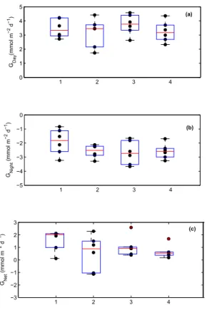
For rubble in ambient seawater conditions, the average G_day, G_night, and G_net in the control experiment were 3.4±0.16 mmol m−2d−1,−2.4±0.15 mmol m−2d−1, and 0.96± 0.20 mmol m−2d−1, respectively. There was no significant difference in Gday (F3,23=

20

(13)

BGD

11, 12799–12831, 2014

dissolution

Title Page

Tables Figures

◭ ◮

Back Close

Full Screen / Esc

Discussion

P

a

per

|

Discus

sion

P

a

per

|

Discussion

P

a

per

|

Discussion

P

a

per

|

3.2 Treatment experiment

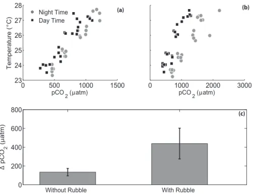
The rubble communities significantly altered the seawater chemistry, with higherpCO2 than the appliedpCO2manipulation, particularly at night (Fig. A1). The mean difference between day and nightpCO₂for all treatments was 134.4±39 µatm without rubble and was 438.5±163.9 µatm when rubble was present (t23=−7.23,p <0.0001; Fig. 2).

5

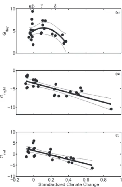
Standardized Climate Change was a significant predictor for Gday, Gnight, and Gnet (Table 2; Fig. 3). G_dayhad a non-linear relationship with Standardized Climate Change (Table 2, Fig. 3a), increasing to a threshold and then rapidly declining. Gnight, however, had a strong linear relationship with Standardized Climate Change (Table 2; Fig. 3b), suggesting that joint increases in ocean pCO₂ and temperature will increase night

10

time dissolution of coral rubble. Lastly, Gnet had a strong negative relationship with Standardized Climate Change (Table 2; Fig. 3c) and the rubble community switched from net calcification to net dissolution at an increase in pCO₂ and temperature of 271.6 µatm and 0.84◦C, respectively.

G and NCP were significantly correlated (p <0.0001, R2=0.85; Figs. 4 and A3).

15

In general, rubble that was net photosynthesizing was also net calcifying and rubble that was net respiring was also net dissolving. The exception was rubble experiencing the most extreme temperature-pCO2treatment, which was net respiring during the day while still holding a positive, yet very low, calcification rate.

4 Discussion

20

4.1 Carbonate chemistry feedbacks

The rubble communities in the aquaria significantly altered the seawater chemistry, particularly at night (t23=−7.23,p <0.0001; Fig. 2, Fig. A1). This day-night difference in seawater chemistry increased under more extreme climate scenarios, as predicted by Jury et al. (2013). This large diel swing inpCO2 is not uncommon on shallow coral

(14)

BGD

11, 12799–12831, 2014

dissolution

Title Page

Tables Figures

◭ ◮

Back Close

Full Screen / Esc

Discussion

P

a

per

|

Discus

sion

P

a

per

|

Discussion

P

a

per

|

Discussion

P

a

per

reef environments.pCO₂ranged from 480 to 975 µatm over 24 h on a shallow reef flat adjacent to our collection site (Silbiger et al., 2014), and pCO2 ranged from 450 to 742 µatm on a Moloka‘i reef flat dominated by coral rubble (Yates and Halley, 2006). Here,pCO₂had an average difference of 438 µatm between day and night with a range of 412 µatm in the pre-industrial treatment to 854 µatm in the most extremepCO2 ×

5

temperature treatments (Fig. 2). In our study, we incorporated these feedbacks into the statistical analysis by using the actual, sampledpCO₂ (and temperature) in each aquaria (Fig. 3) rather than using the intendedpCO2 (and temperature) treatments in an ANOVA (Table A1, Fig. A4), better reflecting thepCO2experienced by organisms in each aquarium.

10

4.2 Calcification and dissolution in a high CO2and temperature environment

Our results suggest that as pCO2 and temperature increase over time, rubble reefs may shift from net calcification to net dissolution. In our study, this tipping point oc-curred at apCO₂ and temperature increase of 271.6 µatm and 0.84◦C. Further, our results showed that Gday and Gnight in a natural coral rubble community have diff

er-15

ent functional responses to changingpCO2 and temperature (Fig. 3). The ranges in G_day and G_night in our aquaria were similar to in situ rates on Hawaiian rubble reefs. Yates and Halley (2006) saw Gday values between 0.26 to 0.98 mmol CaCO3m−

2 h−1 and Gnight values between −0.2 to −3.0 mmol CaCO3 m−

2

h−1 on a Moloka‘i reef flat with only coral rubble. Gdayand Gnightin our experiment ranged from 0.16 to 0.78 and

20

−0.10 to −0.87 mmol CaCO3 m− 2

h−1, respectively, across all treatment conditions. The higher dissolution rates in the in situ study by Yates and Halley (2006) are likely due to dissolution in the sediment, which was not present in our study.

Gday had a non-linear response to Standardized Climate Change. Gday increased withpCO₂×temperature until slightly above ambient conditions, and then decreased

25

(15)

BGD

11, 12799–12831, 2014

dissolution

Title Page

Tables Figures

◭ ◮

Back Close

Full Screen / Esc

Discussion

P

a

per

|

Discus

sion

P

a

per

|

Discussion

P

a

per

|

Discussion

P

a

per

|

We suggest two possible mechanisms to explain why calcification increases in slightly higher pCO2 × temperature than ambient conditions. (1) Some calcifiers can main-tain and even increase their calcification rates in acidic conditions (Kamenos et al., 2013; Findlay et al., 2011; Rodolfo-Metalpa et al., 2011; Martin et al., 2013) by ei-ther modifying their local pH environment (Hurd et al., 2011) or partitioning their

en-5

ergetic resources towards calcification (Kamenos et al., 2013). For example, in low, stable pH conditions the coralline algae,Lithothamnion glaciale, increased its calcifi-cation rate relative to a control treatment but did not concurrently increase its rate of photosynthesis (Kamenos et al., 2013). Kamenos et al. (2013) suggest that the up-regulation of calcification may limit photosynthetic efficiency. In the present study, the

10

increase in G_day coincided with a decrease in net photosynthesis. Photosynthesizing calcifiers in the community may be partitioning their energetic resources more towards calcification and away from photosynthesis in order to maintain a positive calcification rate (Kamenos et al., 2013). (2) An alternative hypothesis is that the calcifiers may be adapted or acclimatized to highpCO2 conditions (Johnson et al., 2014) and have not

15

yet reached their threshold because the rubble was collected from a naturally high and variablepCO₂environment (Guadayol et al., 2014).

We saw a decline in calcification and photosynthesis in the extremepCO2× temper-ature condition. In prior studies, calcification has been shown to decline with climate stressors and the magnitude of decline differs across species (Kroeker et al., 2010;

20

Pandolfi et al., 2011; Ries et al., 2009; Kroeker et al., 2013). The concurrent decline in photosynthesis and calcification (Figs. 3a and 4) suggests that non-photosynthesizing invertebrates in the community (such as bivalves) might be dominating the calcification signal in these conditions. This hypothesis would explain the pattern that we see in Fig. 4, where communities in the most extremepCO2 and temperature conditions are

25

(16)

BGD

11, 12799–12831, 2014

dissolution

Title Page

Tables Figures

◭ ◮

Back Close

Full Screen / Esc

Discussion

P

a

per

|

Discus

sion

P

a

per

|

Discussion

P

a

per

|

Discussion

P

a

per

individual bioeroder taxa have also found higher rates of bioerosion or dissolution in more acidic, higher temperature conditions (Wisshak et al., 2013; Fang et al., 2013; Reyes-Nivia et al., 2013; Tribollet et al., 2009; Wisshak et al., 2012). Studies, including the present one, that focused on community-level responses have consistently found that ocean acidification will increase dissolution rates on coral reefs (Andersson and

5

Gledhill, 2013).

Dissolution was more strongly affected by Standardized Climate Change than calci-fication: this result is not surprising. Bioerosion, an important driver of dissolution, may be more sensitive to changes in ocean acidity than calcification, leading to net dissolu-tion in high CO₂waters. Many boring organisms excrete acidic compounds, which may

10

be less metabolically costly in a low pH environmen. Erez et al. (2011) hypothesize that increased dissolution, rather than decreased calcification, maybe be the reason that net coral reef calcification is sensitive to ocean acidification. The results of this study support this hypothesis. Although G_netdeclines linearly withpCO₂-temperature, calcification (Gday) and dissolution (Gnight) have distinct responses to Standardized

Cli-15

mate Change. Our results highlight the need to study the effects of climate stressors on both calcification and dissolution.

Author contribution. Conceived and designed the experiments: NJS MJD. Performed the ex-periments: NJS. Analyzed the data: NJS MJD. Wrote the paper: NJS MJD.

Acknowledgement. Thanks to I. Caldwell, R. Coleman, J. Faith, K. Hurley, J. Miyano, R.

20

Maguire, D. Schar, J. Sziklay, and M. M. Walton for help in field collections and lab analyses and to R. Briggs from UH SOEST Lab for Analytical Chemistry. M. J. Atkinson, R. Gates, C. Jury, H. Putnam, and R. Toonen gave thoughtful advice throughout the project. Comments by F. Mackenzie improved this manuscript. This project was supported by a NOAA Nancy Foster Scholarship to N. J. S., a PADI Foundation Grant to N. J. S., and Hawaii SeaGrant 1847 to MJD.

25

(17)

BGD

11, 12799–12831, 2014

dissolution

Title Page

Tables Figures

◭ ◮

Back Close

Full Screen / Esc

Discussion

P

a

per

|

Discus

sion

P

a

per

|

Discussion

P

a

per

|

Discussion

P

a

per

|

References

Andersson, A. J. and Gledhill, D.: Ocean acidification and coral reefs: effects on breakdown, dissolution, and net ecosystem calcification, Ann. Rev. Mar. Sci., 5, 321–348, 2013.

Andersson, A. J. and Mackenzie, F. T.: Revisiting four scientific debates in ocean acidification research, Biogeosciences, 9, 893–905, doi:10.5194/bg-9-893-2012, 2012.

5

Andersson, A. J., Kuffner, I. B., Mackenzie, F. T., Jokiel, P. L., Rodgers, K. S., and Tan, A.: Net Loss of CaCO₃ from a subtropical calcifying community due to seawater acidification: mesocosm-scale experimental evidence, Biogeosciences, 6, 1811–1823, doi:10.5194/bg-6-1811-2009, 2009.

Andersson, A. J., Mackenzie, F. T., and Gattuso, J.-P.: Effects of ocean acidification on benthic

10

processes, organisms, and ecosystems, in: Ocean Acidification, edited by: Gattuso, J.-P. and Hansson, L., Oxford University Press, Oxford, 122–153, 2011.

Bopp, L., Resplandy, L., Orr, J. C., Doney, S. C., Dunne, J. P., Gehlen, M., Halloran, P., Heinze, C., Ilyina, T., Séférian, R., Tjiputra, J., and Vichi, M.: Multiple stressors of ocean ecosys-tems in the 21st century: projections with CMIP5 models, Biogeosciences, 10, 6225–6245,

15

doi:10.5194/bg-10-6225-2013, 2013.

Caldeira, K. and Wickett, M. E.: Oceanography: anthropogenic carbon and ocean pH, Nature, 425, 365–365, 2003.

Comeau, S., Edmunds, P. J., Spindel, N. B., and Carpenter, R. C.: The responses of eight coral reef calcifiers to increasing partial pressure of CO₂ do not exhibit a tipping point, Limnol.

20

Oceanogr, 58, 388–398, 2013.

Cubasch, U., Wuebbles, D., Chen, D., Facchini, M. C., Frame, D., Mahowald, N., and Winther, J.-G.: Climate Change 2013: The Physical Science Basis. Contribution of Working Group I to the Fifth Assessment Report of the Intergovernmental Panel on Climate Change Cambridge, UK and New York, NY, USA, 2013.

25

Diaz-Pulido, G., Anthony, K., Kline, D. I., Dove, S., and Hoegh-Guldberg, O.: Interactions be-tween ocean acidification and warming on the mortality and dissolution of coralline alge, J. Phycol., 48, 32–39, 2012.

Dickson, A. G.: Standard potential of the reaction: AgCl (s)+12H₂(g)=Ag (s)+HCl (aq), and and the standard acidity constant of the ion HSO−₄ in synthetic sea water from 273.15 to

30

(18)

BGD

11, 12799–12831, 2014

dissolution

Title Page

Tables Figures

◭ ◮

Back Close

Full Screen / Esc

Discussion

P

a

per

|

Discus

sion

P

a

per

|

Discussion

P

a

per

|

Discussion

P

a

per

Dickson, A. G. and Millero, F. J.: A comparison of the equilibrium constants for the dissociation of carbonic acid in seawater media, Deep-Sea Res. Pt.I, 34, 1733–1743, 1987.

Dickson, A. G., Sabine, C. L., and Christian, J. R.: Guide to best practices for ocean CO₂ measurements, PICES Special Publication 3, 191 pp., 2007.

Doney, S. C., Fabry, V. J., Feely, R. A., and Kleypas, J. A.: Ocean acidification: the other CO₂

5

problem, Ann. Rev. Mar. Sci., 1, 169–192, 2009.

Drupp, P. S., De Carlo, E. H., Mackenzie, F. T., Sabine, C. L., Feely, R. A., and Sham-berger, K. E.: Comparison of CO₂dynamics and air–sea gas exchange in differing tropical reef environments, Aquatic Geochem., 19, 371–397, 2013.

Erez, J., Reynaud, S., Silverman, J., Schneider, K., and Allemand, D.: Coral calcification under

10

ocean acidification and global change, in: Coral Reefs: an Ecosystem in Transition, edited by: Dubinski, Z., and Stambler, N., Springer, 151–176, 2011.

Fabricius, K. E.: Effects of terrestrial runoffon the ecology of corals and coral reefs: review and synthesis, Mar. Pollut. Bull., 50, 125–146, 2005.

Fabricius, K., Langdon, C., Uthicke, S., Humphrey, C., Noonan, S., De’ath, G., Okazaki, R.,

15

Muehllehner, N., Glas, M., and Lough, J.: Losers and winners in coral reefs acclimatized to elevated carbon dioxide concentrations, Nature Climate Change, 1, 165–169, 2011.

Fair, R. C.: On the robust estimation of econometric models, Ann. Econ. Soc. Meas., 3, 117– 128, 1974.

Fang, J. K. H., Mello-Athayde, M. A., Schönberg, C. H. L., Kline, D. I., Hoegh-Guldberg, O.,

20

and Dove, S.: Sponge biomass and bioerosion rates increase under ocean warming and acidification, Global Change Biol., 19, 3581–3591, 2013.

Fangue, N. A., O’Donnell, M. J., Sewell, M. A., Matson, P. G., MacPherson, A. C., and Hof-mann, G. E.: A laboratory-based, experimental system for the study of ocean acidification effects on marine invertebrate larvae, Limnol. Oceanogr. Methods, 8, 441–452, 2010.

25

Feely, R. A., Sabine, C. L., Lee, K., Berelson, W., Kleypas, J., Fabry, V. J., and Millero, F. J.: Impact of anthropogenic CO₂on the CaCO₃system in the oceans, Science, 305, 362–366, 2004.

Findlay, H. S., Wood, H. L., Kendall, M. A., Spicer, J. I., Twitchett, R. J., and Widdicombe, S.: Comparing the impact of high CO₂ on calcium carbonate structures in different marine

or-30

(19)

BGD

11, 12799–12831, 2014

dissolution

Title Page

Tables Figures

◭ ◮

Back Close

Full Screen / Esc

Discussion

P

a

per

|

Discus

sion

P

a

per

|

Discussion

P

a

per

|

Discussion

P

a

per

|

Gattuso, J.-P., Frankignoulle, M., and Smith, S. V.: Measurement of community metabolism and significance in the coral reef CO₂ source-sink debate, Proc. Natl. Acad. Sci., 96, 13017– 13022, 1999.

Guadayol, Ò., Silbiger, N. J., Donahue, M. J., and Thomas, F. I. M.: Patterns in temporal vari-ability of temperature, oxygen and pH along an environmental gradient in a coral reef, PloS

5

one, 9, e85213, doi:10.1371/journal.pone.0085213, 2014.

Hoegh-Guldberg, O. and Bruno, J. F.: The impact of climate change on the world’s marine ecosystems, Science, 328, 1523–1528, 2010.

Hoegh-Guldberg, O., Mumby, P. J., Hooten, A. J., Steneck, R. S., Greenfield, P., Gomez, E., Harvell, C. D., Sale, P. F., Edwards, A. J., Caldeira, K., Knowlton, N., Eakin, C. M.,

Iglesias-10

Prieto, R., Muthiga, N., Bradbury, R. H., Dubi, A., and Hatziolos, M. E.: Coral reefs under rapid climate change and ocean acidification, Science, 318, 1737–1742, 2007.

Hurd, C. L., Cornwall, C. E., Currie, K., Hepburn, C. D., McGraw, C. M., Hunter, K. A., and Boyd, P. W.: Metabolically induced pH fluctuations by some coastal calcifiers exceed pro-jected 22nd century ocean acidification: a mechanism for differential susceptibility?, Glob.

15

Change Biol., 17, 3254–3262, 2011.

Johnson, M. D. and Carpenter, R. C.: Ocean acidification and warming decrease calcification in the crustose coralline algaHydrolithon onkodesand increase susceptibility to grazing, J. Exp. Mar. Biol. Ecol., 434, 94–101, 2012.

Johnson, M. D., Moriarty, V. W., and Carpenter, R. C.: Acclimatization of the

crus-20

tose coralline alga Porolithon onkodes to variable pCO₂, PLOS ONE, 9, e87678, doi:10.1371/journal.pone.0087678, 2014.

Jokiel, P. L., Rodgers, K. S., Kuffner, I. B., Andersson, A. J., Cox, E. F., and Mackenzie, F. T.: Ocean acidification and calcifying reef organisms: a mesocosm investigation, Coral Reefs, 27, 473–483, 2008.

25

Jury, C. P., Thomas, F. I. M., Atkinson, M. J., and Toonen, R. J.: Buffer capacity, ecosystem feedbacks, and seawater chemistry under global change, Water, 5, 1303–1325, 2013. Kamenos, N. A., Burdett, H. L., Aloisio, E., Findlay, H. S., Martin, S., Longbone, C., Dunn, J.,

Widdicombe, S., and Calosi, P.: Coralline algal structure is more sensitive to rate, rather than the magnitude, of ocean acidification, Global Change Biology, 19, 3621–3628, 2013.

30

(20)

BGD

11, 12799–12831, 2014

dissolution

Title Page

Tables Figures

◭ ◮

Back Close

Full Screen / Esc

Discussion

P

a

per

|

Discus

sion

P

a

per

|

Discussion

P

a

per

|

Discussion

P

a

per

Kroeker, K. J., Kordas, R. L., Crim, R. N., and Singh, G. G.: Meta-analysis reveals negative yet variable effects of ocean acidification on marine organisms, Ecol. Lett., 13, 1419–1434, 2010.

Kroeker, K. J., Kordas, R. L., Crim, R., Hendriks, I. E., Ramajo, L., Singh, G. S., Duarte, C. M., and Gattuso, J. P.: Impacts of ocean acidification on marine organisms: quantifying

sensitiv-5

ities and interaction with warming, Glob. Change Biol., 19, 1884–1896, 2013.

Lowe, R. J., Falter, J. L., Monismith, S. G., and Atkinson, M. J.: A numerical study of circulation in a coastal reef-lagoon system, J. Geophys. Res.-Oceans, 114, C06022, doi:10.1029/2008JC005081, 2009a.

Lowe, R. J., Falter, J. L., Monismith, S. G., and Atkinson, M. J.: Wave-driven circulation of

10

a coastal reef-lagoon system, J. Phys. Oceanogr., 39, 873–893, 2009b.

Martin, S., Cohu, S., Vignot, C., Zimmerman, G., and Gattuso, J. P.: One-year experiment on the physiological response of the Mediterranean crustose coralline alga, Lithophyllum cabiochae, to elevatedpCO₂and temperature, Ecol. Evol., 3, 676–693, 2013.

Mehrbach, C.: Measurement of the apparent dissociation constants of carbonic acid in seawater

15

at atmospheric pressure, Limnol. Oceanogr., 18, 897–907, 1973.

Meinshausen, M., Smith, S. J., Calvin, K., Daniel, J. S., Kainuma, M. L. T., Lamarque, J. F., Matsumoto, K., Montzka, S. A., Raper, S. C. B., and Riahi, K.: The RCP greenhouse gas concentrations and their extensions from 1765 to 2300, Clim. Change, 109, 213–241, 2011. Pandolfi, J. M., Connolly, S. R., Marshall, D. J., and Cohen, A. L.: Projecting coral reef futures

20

under global warming and ocean acidification, Science, 333, 418–422, 2011.

Reyes-Nivia, C., Diaz-Pulido, G., Kline, D., Guldberg, O.-H., and Dove, S.: Ocean acidification and warming scenarios increase microbioerosion of coral skeletons, Glob. Change Biol., 19, 1919–1929, 2013.

Ries, J. B., Cohen, A. L., and McCorkle, D. C.: Marine calcifiers exhibit mixed responses to

25

CO₂-induced ocean acidification, Geology, 37, 1131–1134, 2009.

Rodolfo-Metalpa, R., Houlbrèque, F., Tambutté, É., Boisson, F., Baggini, C., Patti, F. P., Jef-free, R., Fine, M., Foggo, A., and Gattuso, J. P.: Coral and mollusc resistance to ocean acidification adversely affected by warming, Nature Clim. Change, 1, 308–312, 2011. Rogelj, J., Meinshausen, M., and Knutti, R.: Global warming under old and new scenarios using

30

IPCC climate sensitivity range estimates, Nature Clim. Change, 2, 248–253, 2012.

(21)

dan-BGD

11, 12799–12831, 2014

dissolution

Title Page

Tables Figures

◭ ◮

Back Close

Full Screen / Esc

Discussion

P

a

per

|

Discus

sion

P

a

per

|

Discussion

P

a

per

|

Discussion

P

a

per

|

Semesi, I. S., Kangwe, J., and Björk, M.: Alterations in seawater pH and CO₂affect calcification and photosynthesis in the tropical coralline alga,Hydrolithon sp. (Rhodophyta), Estuarine, Coast. Shelf Sci., 84, 337–341, 2009.

Silbiger, N. J., Guadayol, Ò., Thomas, F. I. M., and Donahue M. J.: Reefs shift from net accretion to net erosion along a natural environmental gradient, Mar. Ecol. Progress Ser., in press,

5

2014.

Smith, S. V. and Key, G. S.: Carbon dioxide and metabolism in marine environments, Limnol. Oceanogr, 20, 493–495, 1975.

Smith, S. V., Kimmerer, W. J., Laws, E. A., Brock, R. E., and Walsh, T. W.: Kaneohe Bay sewage diversion experiment-perspectives on ecosystem responses to nutritional perturbation, Pacif.

10

Sci., 35, 279–402, 1981.

Stimson, J. and Kinzie III, R. A.: The temporal pattern and rate of release of zooxanthellae from the reef coralPocillopora damicornis(Linnaeus) under nitrogen-enrichment and control conditions, J. Exp. Mar. Biol. Ecol., 153, 63–74, 1991.

Tans, P. and Keeling, R.: NOAA/ESRL, available at: www.esrl.noaa.gov/gmd/ccgg/trends/,

15

2013.

Tribollet, A., and Payri, C.: Bioerosion of the coralline algaHydrolithon onkodesby microborers in the coral reefs of Moorea, French Polynesia, Oceanol. Acta, 24, 329–342, 2001.

Tribollet, A., Atkinson, M. J., and Langdon, C.: Effects of elevatedpCO₂ on epilithic and en-dolithic metabolism of reef carbonates, Glob. Change Biol., 12, 2200–2208, 2006.

20

Tribollet, A., Godinot, C., Atkinson, M., and Langdon, C.: Effects of elevatedpCO₂on dissolution of coral carbonates by microbial euendoliths, Global Biogeochem. Cy., 23, GB3008, 2009. Uppström, L. R.: The boron/chlorinity ratio of deep-sea water from the Pacific Ocean, Deep

Sea Research and Oceanographic Abstracts, 1974, 161–162.

Van Heuven, S., Pierrot, D., Lewis, E., and Wallace, D. W. R.: MATLAB Program developed for

25

CO₂system calculations, Rep. ORNL/CDIAC-105b, 2009.

Van Vuuren, D. P., Meinshausen, M., Plattner, G. K., Joos, F., Strassmann, K. M., Smith, S. J., Wigley, T. M. L., Raper, S. C. B., Riahi, K., and De La Chesnaye, F.: Temperature increase of 21st century mitigation scenarios, Proc. Natl. Acad. Sci., 105, 15258–15262, 2008.

Van Vuuren, D. P., Edmonds, J., Kainuma, M., Riahi, K., Thomson, A., Hibbard, K., Hurtt, G. C.,

30

(22)

BGD

11, 12799–12831, 2014

dissolution

Title Page

Tables Figures

◭ ◮

Back Close

Full Screen / Esc

Discussion

P

a

per

|

Discus

sion

P

a

per

|

Discussion

P

a

per

|

Discussion

P

a

per

White, J.: Distribution, recruitment and development of the borer community in dead coral on shallow Hawaiian reefs, Ph. D., Zoology, University of Hawaii at Manoa, Honolulu, 1980. Wisshak, M., Schönberg, C. H. L., Form, A., and Freiwald, A.: Ocean acidification accelerates

reef bioerosion, Plos One, 7, e45124–e45124, 2012.

Wisshak, M., Schönberg, C. H. L., Form, A., and Freiwald, A.: Effects of ocean acidification and

5

global warming on reef bioerosion – lessons from a clionaid sponge, Aq. Biol., 19, 111–127, 2013.

Yates, K. K. and Halley, R. B.: CO₃2− concentration andpCO₂ thresholds for calcification and dissolution on the Molokai reef flat, Hawaii, Biogeosciences, 3, 357–369, doi:10.5194/bg-3-357-2006, 2006.

(23)

BGD

11, 12799–12831, 2014

dissolution

Title Page

Tables Figures

◭ ◮

Back Close

Full Screen / Esc

Discussion

P

a

per

|

Discus

sion

P

a

per

|

Discussion

P

a

per

|

Discussion

P

a

per

|

Table 1.Means and standard errors of all measured parameters by rack.pCO₂, HCO−₃, CO2₃−, DIC, andΩaragwere all calculated from the measured TA and pH samples using CO2SYS. Data are all from the imposed treatment conditions with no rubble inside the aquaria.

Rack Pre-industrial Present Day 2050 prediction 2100 prediction

Temp (◦C) 23.8±0.07 24.8±0.08 26.2±0.06 27.2±0.08 Salinity (psu) 35.65±0.01 35.71±0.02 35.62±0.02 35.71±0.02 Total Alkalinity (µmol kg−1) 2137±1.7 2138±2.3 2139±2.0 2142±1.9 pH_t 8.02±0.02 7.87±0.01 7.74±0.02 7.67±0.02 pCO₂(µatm) 409±20.0 614±15.6 868±33.0 1047±38.7 HCO−₃(µmol kg−1) 1692±16.9 1815±7.3 1894±7.8 1939±6.6 CO2₃−(µmol kg−1) 194.20±6.7 147.08±2.8 113.98±3.8 99.24±3.3 DIC (µmol kg−1) 1898±10.9 1980±5.1 2032±5.0 2067±4.5

Ωarag 3.06±0.1 2.32±0.04 1.80±0.06 1.57±0.05

(24)

BGD

11, 12799–12831, 2014

dissolution

Title Page

Tables Figures

◭ ◮

Back Close

Full Screen / Esc

Discussion

P

a

per

|

Discus

sion

P

a

per

|

Discussion

P

a

per

|

Discussion

P

a

per

Table 2.Regression results for the treatment experiments:G_day,G_night, andG_netversus Stan-dardized Climate Change (Fig. 3).

SS df F p R2

Gday

Standardized Climate Change 5.82 1 1.97 0.17 (Standardized Climate Change)2 18.67 1 6.33 0.02

Error 61.86 21 2.95 0.29

G_night

Standardized Climate Change 73.60 1 50.09 <0.0001

Error 32.32 22 0.70

G_net

Standardized Climate Change 89.79 1 20.25 <0.001

(25)

BGD

11, 12799–12831, 2014

dissolution

Title Page

Tables Figures

◭ ◮

Back Close

Full Screen / Esc

Discussion

P

a

per

|

Discus

sion

P

a

per

|

Discussion

P

a

per

|

Discussion

P

a

per

|

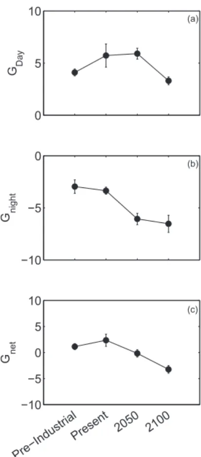
Table A1.Analysis of treatment experiment using an ANOVA design (Appendix Fig. A4).

SS df MS F p

Gday

Groups 28.83 3 9.81 3.65 0.030

Error 52.61 20 2.63 Total 81.45 23

G_night

Groups 60.39 3 20.13 8.84 <0.0001

Error 45.53 20 2.28 Total 105.92 23

Gnet

Groups 104.31 3 34.77 8.37 <0.0001

(26)

BGD

11, 12799–12831, 2014

dissolution

Title Page

Tables Figures

◭ ◮

Back Close

Full Screen / Esc

Discussion

P

a

per

|

Discus

sion

P

a

per

|

Discussion

P

a

per

|

Discussion

P

a

per

Filtered Ambient Seawater

Header Tanks

Individual Aquaria

}

pCO

2

Flow

Temperature

}

Rack

Light

Fig 1

(27)

BGD

11, 12799–12831, 2014

dissolution

Title Page

Tables Figures

◭ ◮

Back Close

Full Screen / Esc

Discussion

P

a

per

|

Discus

sion

P

a

per

|

Discussion

P

a

per

|

Discussion

P

a

per

|

0 500 1000 1500

23 24 25 26 27 28

pCO

2 (µatm)

Temperature (

°

C)

Night Time Day Time

0 1000 2000 3000

pCO

2 (µatm)

Without Rubble With Rubble

0 200 400 600 800

∆

pCO

2

(

µ

atm

)

(a) (b)

(c)

Fig 2

Figure 2.pCO₂and temperature in each aquarium(a)without any rubble present and(b)with rubble present. Daily variability inpCO₂was higher when rubble was present due to feedbacks from the rubble community. (Note the differentxaxis scales in panelsaandb). Panel(c)shows the mean difference between day and nightpCO₂with and without rubble present (error bars are standard error) (t23=−7.23,p <0.0001).

(28)

BGD

11, 12799–12831, 2014

dissolution

Title Page

Tables Figures

◭ ◮

Back Close

Full Screen / Esc

Discussion

P

a

per

|

Discus

sion

P

a

per

|

Discussion

P

a

per

|

Discussion

P

a

per

−0.2 0 0.2 0.4 0.6 0.8 1

−10 −5 0 5 10

Standardized Climate Change Gnet

0 5 10

Gday

αβ γ δ

−10 −5 0

Gnight

(a)

(b)

(c)

Fig. 3

Figure 3. Net ecosystem calcification: (a) Gday, (b) Gnight, and (c) Gnet versus Standardized Climate Change. Each point represents net ecosystem calcification calculated from an indi-vidual aquarium. Standardized Climate Change was centered around background seawater conditions such that a value of 0 indicated that there was no change inpCO₂or temperature. Positive values indicate an elevated pCO₂ and temperature condition relative to background and negative values represent lowerpCO₂and temperature conditions.G_dayhad a non-linear relationship with Standardized Climate Change (y=−1.6×10−8x2+1.4×10−4x+5.5), while

(29)

BGD

11, 12799–12831, 2014

dissolution

Title Page

Tables Figures

◭ ◮

Back Close

Full Screen / Esc

Discussion

P

a

per

|

Discus

sion

P

a

per

|

Discussion

P

a

per

|

Discussion

P

a

per

|

−60 −40 −20 0 20 40 60

−20 −15 −10 −5 0 5 10 15 20

NCP (mmol C m−2 d−1

G (mmol CaCO

3

m

−2 d

−1

Day

)

) Night

Standardized Climate Change

−1 −0.5 0 0.5 1 1.5 2 2.5 3 3.5 4 x 104

Net C

alcifica

tion

Net Photosynthesis

Net Dissolution

Net Respiration

Fig 4

Figure 4.CalculatedG and NCP rates for all treatment aquaria. The color represents Stan-dardized Climate Change. Squares are data collected during the light conditions and circles represent data collected during dark conditions. All negative numbers are either net dissolu-tion or net respiradissolu-tion while positive numbers are net calcificadissolu-tion or net photosynthesis. There is a strong positive relationship betweenGand NCP (y=0.14x+1.9,p <0.0001,R2=0.85). Black and gray lines represent the best-fit line and 95 % confidence intervals, respectively. Sup-plement Fig. A3 is a similar plot with specific aquaria labeled.

(30)

BGD

11, 12799–12831, 2014

dissolution

Title Page

Tables Figures

◭ ◮

Back Close

Full Screen / Esc

Discussion

P

a

per

|

Discus

sion

P

a

per

|

Discussion

P

a

per

|

Discussion

P

a

per

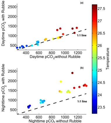
400 600 800 1000 1200

500 1000 1500 2000 2500

Daytime pCO with Rubble

2

Daytime pCO without Rubble₂

400 600 800 1000 1200

500 1000 1500 2000 2500

Nighttime pCO with Rubble

2

Nighttime pCO without Rubble₂

Temperature

23.5 24 24.5 25 25.5 26 26.5 27 27.5

1:1 line

(a)

(b)

(31)

BGD

11, 12799–12831, 2014

dissolution

Title Page

Tables Figures

◭ ◮

Back Close

Full Screen / Esc

Discussion

P

a

per

|

Discus

sion

P

a

per

|

Discussion

P

a

per

|

Discussion

P

a

per

|

0 1 2 3 4 5

1 2 3 4

GDay

(mmol m

−2 d −1)

(a)

−5 −4 −3 −2 −1 0

1 2 3 4

GNight

(mmol m

−2 d

−1) (b)

−3 −2 −1 0 1 2 3

1 2 3 4

(c)

GNet

(mmol m

−2 d −1)

Fig A2

(32)

BGD

11, 12799–12831, 2014

dissolution

Title Page

Tables Figures

◭ ◮

Back Close

Full Screen / Esc

Discussion

P

a

per

|

Discus

sion

P

a

per

|

Discussion

P

a

per

|

Discussion

P

a

per

−50 0 50

−20 −10 0 10 20

1 2 3

4

5 6

7 8 9

10 1112

131415 161718 19 20 21 2422 23

1 2 3 4

5

6

7 ₈

9

10 1112 14 1513 16 1718 19

20 21 2223 24

NCP mmol C m−2 d−1

G (mmol CaCO

3

m

−2 d

−1 Day

)

Night

1900 2000 2100 2200 2300

2100 2150 2200 2250 2300 2350

DIC₃₅µmol kg−1

TA

35

(µ

mol kg

−1

(a)

(b)

Fig A3

(33)

BGD

11, 12799–12831, 2014

dissolution

Title Page

Tables Figures

◭ ◮

Back Close

Full Screen / Esc

Discussion

P

a

per

|

Discus

sion

P

a

per

|

Discussion

P

a

per

|

Discussion

P

a

per

|

0 5 10

G Day

−10 −5

0

G night

−10 −5

0 5 10

G net

Pre−Industrial

Present 2050 2100

(a)

(b)

(c)

Fig A4

Figure A4.Means and standard error bars for(a)G_day,(b)G_night, and(c)G_netin mmol m−2d−1.