www.atmos-meas-tech.net/3/283/2010/
© Author(s) 2010. This work is distributed under the Creative Commons Attribution 3.0 License.
Measurement
Techniques
Retrieval of tropospheric column densities of NO
2
from combined
SCIAMACHY nadir/limb measurements
S. Beirle, S. K ¨uhl, J. Puk¸¯ıte, and T. Wagner
Max-Planck-Institut f¨ur Chemie, Mainz, Germany
Received: 6 November 2009 – Published in Atmos. Meas. Tech. Discuss.: 23 November 2009 Revised: 16 February 2010 – Accepted: 23 February 2010 – Published: 25 February 2010
Abstract. The SCIAMACHY instrument onboard the ESA satellite ENVISAT allows measurements of various atmo-spheric trace gases, such as NO2. A unique feature of SCIA-MACHY is that measurements are made alternately in limb and nadir mode. The limb measurements provide an oppor-tunity for directly determining stratospheric column densities (CDs), which are needed to extract tropospheric CDs from the total CD measurements performed in (quasi simultane-ous) nadir geometry.
Here we discuss the potential and limitations of SCIA-MACHY limb measurements for estimating stratospheric CDs of NO2 in comparison to a simple reference sector method, and the consequences for the resulting tropospheric CDs. A direct, absolute limb correction scheme is presented that improves spatial patterns of tropospheric NO2column densities at high latitudes, but results in artificial zonal stripes at low latitudes. Subsequently, a relative limb correction scheme is introduced that successfully reduces stratospheric artefacts in the tropospheric data product without introducing new ones. This relative limb correction scheme is rather sim-ple, robust, and, in essence, based on measurements alone.
The effects of the different stratospheric estimation schemes on tropospheric CDs are discussed with respect to zonal and temporal dependencies. In addition, we define er-ror quantities from the nadir/limb measurements that indicate remaining systematic errors as a function of latitude and day. Our new suggested stratospheric estimation scheme, the relative limb correction, improves mean tropospheric slant CDs significantly, e.g. from−1×10¹⁵molec/cm2 (using a reference sector method) to≈0 in the Atlantic ocean, and from+1×10¹⁵molec/cm2 to≈0 over Siberia, at 50◦
N in January 2003–2008.
Correspondence to:S. Beirle ([email protected])
1 Introduction
Satellite-borne UV-vis spectrometers, like the Global Ozone Monitoring Experiment (GOME 1 & 2), the SCanning Imag-ing Absorption spectroMeter for Atmospheric CHartogra-phY (SCIAMACHY), or the Ozone Monitoring Instrument (OMI) (e.g. Burrows et al., 1999; Bovensmann et al., 1999; Levelt et al., 2006), originally designed for monitoring stratospheric ozone, are also used for the retrieval of other at-mospheric trace gases like NO2, SO2, H2O, OClO, BrO, IO, HCHO, or CHOCHO, on global scale (e.g. Burrows et al., 1999; Martin et al., 2008; Wagner et al., 2008). In particular the retrieval of tropospheric NO2column densities has been demonstrated and analyzed in several studies with numerous scientific applications in recent years (see for instance Martin et al., 2008, and references therein).
From the spectrally resolved nadir measurements, total slant column densities (SCDs), i.e. concentrations integrated along the effective light path, are derived by differential opti-cal absorption spectroscopy (DOAS) (Platt and Stutz, 2008) or similar techniques. SCDs can be transformed to vertical column densities (VCDs) by accounting for radiative trans-fer in the atmosphere. Note that in the following we use the inspecific term “column densities” (CDs), but define and dis-cuss the matter of vertical versus slant column densities in detail in Sects. 2.4 and 2.5.
In this study, we focus on stratospheric estimation schemes (SES) for NO2. The choice of the SES has significant im-pact on the retrieved tropospheric CDs of NO2and leads to systematic differences between retrieval schemes. Generally, there are three approaches for the estimation of stratospheric CDs, using (1) atmospheric chemistry models, (2) a subset of the satellite measurements which are assumed to be free of tropospheric pollution, and (3) additional (more or less) direct measurements of the stratospheric CD.
(1) Atmospheric chemistry models directly provide infor-mation on stratospheric CDs which can be used for the re-trieval of tropospheric CDs. Richter et al. (2005) take strato-spheric CDs of NO2 from the SLIMCAT model for their stratospheric estimation. Boersma et al. (2007) use a data assimilation approach with the TM4 model.
While stratospheric NOx chemistry is in general under-stood quite well, the utilization of chemistry models for the stratospheric estimation nevertheless has its drawbacks. First, models and measurements are generally not in perfect agreement, but have systematic biases dependent on time, latitude, and/or observation geometry. Hence, model CDs have to be “tuned” – somewhat arbitrarily – to match obser-vations (see Richter et al., 2005). Second, in the case of data assimilation, a-priori knowledge on the global tropospheric NO2distribution is needed; in case of a (faulty) stratospheric classification of a signal of tropospheric origin, it would be assimilated in the stratosphere. Third, the resulting tropo-spheric CDs are not independent measurements any more.
(2) In several stratospheric correction schemes the satellite measurements themselves are used to define subsets of data that are assumed to represent the stratospheric CD. These subsets are inter- or extrapolated to global fields afterwards.
A quite simple stratospheric correction scheme for NO2 is the reference sector method (RSM) (e.g. Richter and Bur-rows, 2002; Martin et al., 2002; Beirle et al., 2003): The stratospheric CD at a given latitude is estimated from mea-surements over the remote Pacific (at the respective latitude), which can be considered to be unpolluted. Note that this approach is only applicable for satellites operated in sun-synchonous orbit, so that thelocaltime of measurements in-and outside the reference sector is the same. The RSM gen-erally results in troposphericexcessCDs w.r.t. the reference sector. Within the RSM approach, longitudinal variations of stratospheric NO2are neglected, which generally works well for low and mid-latitudes, but may fail especially at higher latitudes, in particular close to the polar vortices (e.g. Richter and Burrows, 2002; Martin et al., 2002; Boersma et al., 2004; Sierk et al., 2006).
Some refinements of the simple RSM have been dis-cussed, which take longitudinal variations of stratospheric CDs into account, but still estimate them from the measure-ments alone. Leue et al. (2001) and Wenig et al. (2004) de-fine unpolluted reference regions around the globe (instead of just one band in the Pacific) and interpolate the strato-spheric 2-FD field. Bucsela et al. (2006) perform a Wave-2
fitting along zonal bands. While these refined RSM methods account for longitudinal variations, they require the (rather arbitrary) selection of “unpolluted” regions which must nei-ther be too small (which could lead to interpolation errors and possibly to overshoots of the interpolated stratosphere over the large “polluted” area) nor too large (which could lead to the false classification of a smooth continental tro-pospheric background in the “unpolluted” region, e.g. from soil emissions, as stratospheric NO2). These difficulties are amplified in the case of SCIAMACHY due to its poor spatial coverage (compared to GOME/GOME-2 or OMI).
(3) SCIAMACHY is the first satellite instrument that com-bines limb and nadir measurements. The viewing geome-try alternates between nadir and limb states in such a way, that the atmosphere is first scanned in limb (allowing the re-trieval of stratospheric profiles), and subsequently in nadir geometry (providing total CDs for approximately the same air mass) (see Bovensmann et al., 1999). This “Limb-Nadir-Matching” was intended to provide direct measurements of stratospheric CDs corresponding to the successive nadir CD measurements.
For NO2 and O3, the potential of SCIAMACHY limb measurements for stratospheric correction has already been demonstrated exemplarily (Sioris et al., 2004; PROMOTE, 2004; Sierk et al., 2006; Heckel et al., 2007). However, to the authors’ knowledge, no standard data product of tro-pospheric NO2is currently retrieved utilizing limb data for stratospheric correction.
studies (like emission estimates) based on NO2 CDs from satellite measurements.
2 Data and methods
In this section we shortly describe the characteristics of the SCIAMACHY instrument (Sect. 2.1) and our retrieval schemes of NO2 nadir CDs (Sect. 2.2) and limb profiles (Sect. 2.3).
We discuss different stratospheric estimation schemes (SES) in Sect. 2.4: first (Sect. 2.4.1) the simple reference sector method (RSM), second (Sect. 2.4.2), an absolute limb correction (ALC) scheme, and third (Sect. 2.4.3), a relative limb correction (RLC) scheme. From these three strato-spheric estimation schemes, we accordingly derive three tro-pospheric products (Sect. 2.5), which are compared and dis-cussed in Sects. 3 (results) and 4 (discussion).
In Sect. 2.6 we discuss to which extent information on sta-tistical as well as systematic errors of tropospheric CDs can be gained from the limb/nadir measurements themselves.
The different SES are illustrated exemplarily for 28 Jan-uary 2006. Additional examples for other times of the year, as well as a more in-depth discussion of error quantities, are presented in a supplementary document, referred to as “Sup-plement” hereafter (see http://www.atmos-meas-tech.net/3/ 283/2010/amt-3-283-2010-supplement.pdf).
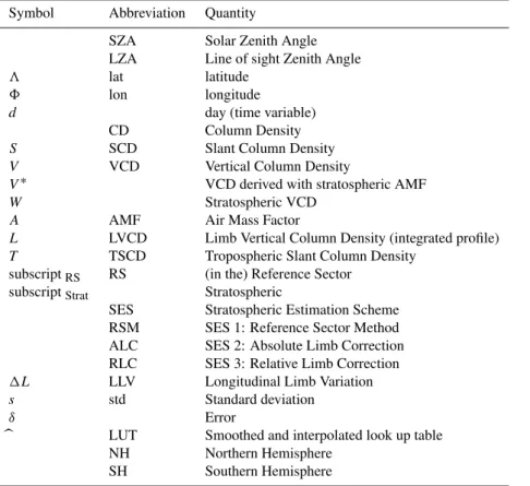
Table 1 gives an overview on the symbols and abbrevia-tions used in this study.
2.1 SCIAMACHY
The Scanning Imaging Absorption spectroMeter for Atmo-spheric CHartographY, SCIAMACHY (Bovensmann et al., 1999), was launched onboard the ESA satellite ENVISAT in March 2002. ENVISAT orbits the Earth in a sun-synchronous orbit with an inclination from the equatorial plane of 98.5◦. It performs one orbit in approx. 100 min, with a local equator crossing time of about 10:00 a.m. in de-scending node.
SCIAMACHY measures Earthshine spectra from the UV to the NIR with a spectral resolution of 0.22–1.48 nm. It is operated in different viewing geometries, including nadir, limb, and solar/lunar occultation. In nadir geometry (i.e. di-rected vertically, perpendicular to the Earth’s surface), the instrument performs an across-track scan of about ±32◦, equivalent to a swath-width of 960 km. The footprint of a sin-gle nadir observation is typically 30×60 km2. Global cover of nadir measurements is achieved after 6 days. In limb ge-ometry (i.e. directed horizontally, tangential to the Earth’s surface), the instrument performs scans in flight direction with elevation steps of approx. 3.3 km at the tangent point. The cross-track swath is 960 km, as for the nadir measure-ments, and consists of up to 4 pixels. The field of view at the
tangent point is about 2.5 km (vertically)×110 km (horizon-tally). The limb scanning allows the retrieval of stratospheric profiles of NO2(see Sect. 2.3).
In standard operation, the measurement state alternates be-tween limb and nadir in such a way that the limb measure-ments probe (almost) the same stratospheric air mass as the subsequent nadir measurements. Note that the term “state” in the following is used to denote the SCIAMACHY surement mode as well as to summarize the entity of mea-surements performed within one nadir/limb state.
2.2 Retrieval of total slant column densities of NO2:
nadir
Slant column densities (SCDs)S of NO2 are derived from SCIAMACHY nadir spectra using Differential Optical Ab-sorption Spectroscopy DOAS (Platt and Stutz, 2008). Cross-sections of O3, NO2, O4, H2O and CHOCHO are fitted in the spectral range 430.8–459.5 nm. In addition, Ring spectra, ac-counting for inelastic scattering in the atmosphere (rotational Raman) as well as in liquid water (vibrational Raman), an absorption cross-section of liquid water, and a polynomial of degree 5 are included in the fit procedure. A daily solar measurement is used as Fraunhofer reference spectrum.
This NO2 DOAS retrieval setup is different from previ-ous versions (e.g. Beirle, 2004) in so far that liquid water absorption and vibrational Raman scattering on liquid wa-ter molecules, which have been shown to affect spectra in the UV/vis (Vasilkov et al., 2002; Vountas et al., 2007), is now accounted for. This modification improves the spectral fits over oligotrophic oceanic regions (Polovina et al., 2008), where NO2SCDs of the previous fit version show a system-atic negative bias. The remaining (but significantly smaller) systematic spatial patterns over oligotrophic oceanic regions are subject to further investigations. These effects are related to this study in that large parts of the chosen reference region in the Pacific cover oligotrophic regions. With the current settings, the remaining biases over oceans are rather small (see discussion). Information on statistical and possible sys-tematic fit errors can be derived from the standard deviation of NO2CDs in the reference sector (RS) (see Sect. 2.6).
In the DOAS set-up, a single NO2cross-section for a tem-perature of 220 K is included (Vandaele et al., 1998), which is appropriate for the stratosphere. Tropospheric CDs have to be corrected by a factor of about 1.2, to account for the tem-perature dependency of the NO2cross-section (see Boersma et al., 2004).
Table 1.Abbreviations and Variables used in this study.
Symbol Abbreviation Quantity
SZA Solar Zenith Angle LZA Line of sight Zenith Angle 3 lat latitude
8 lon longitude
d day (time variable) CD Column Density S SCD Slant Column Density V VCD Vertical Column Density
V∗ VCD derived with stratospheric AMF W Stratospheric VCD
A AMF Air Mass Factor
L LVCD Limb Vertical Column Density (integrated profile) T TSCD Tropospheric Slant Column Density
subscriptRS RS (in the) Reference Sector subscriptStrat Stratospheric
SES Stratospheric Estimation Scheme RSM SES 1: Reference Sector Method ALC SES 2: Absolute Limb Correction RLC SES 3: Relative Limb Correction 1L LLV Longitudinal Limb Variation s std Standard deviation
δ Error
b LUT Smoothed and interpolated look up table NH Northern Hemisphere
SH Southern Hemisphere
2.3 Retrieval of stratospheric NO2profiles: limb
An algorithm for the retrieval of NO2, BrO and OClO verti-cal profiles from SCIAMACHY limb measurements was de-veloped in our group (Puk¸¯ıte et al., 2006; K¨uhl et al., 2008). The retrieval is performed in two steps: In the first step, SCDs are derived from the SCIAMACHY limb spectra at different tangent heights by DOAS. For NO2the fit-window ranges from 420 to 450 nm. The NO2cross-section at 223 K is taken from Bogumil et al. (2003). As reference spec-trum we use a measurement at a tangent height where the absorption of the considered trace gas is small, i.e. for NO2 at∼42 km.
Second, the trace gas SCDs are converted into a verti-cal concentration profile by an inversion scheme based on a least squares approach (see e.g. Menke, 1999). To increase the signal-to-noise ratio, only one averaged SCD per tangent height is applied for the inversion (i.e. the SCD results of the four measured spectra per tangent height are co-added).
For the inversion, box air mass factors (AMFs) are cal-culated with the 3-D fully spherical Monte Carlo radiative transfer model (RTM) “McArtim” (Deutschmann, 2009), us-ing temperature, pressure and ozone data from a model sim-ulation provided by Br¨uhl and Crutzen (1993). It should be noted that in some individual cases the actual temperature, pressure and ozone profile might differ considerably from the
assumed model profiles. No aerosols and clouds are assumed for the calculation of the box AMFs. The aerosol extinction is much lower compared to extinction by Rayleigh scattering in the stratosphere. Also, due to the limb viewing geometry and the narrow field of view, SCDs derived from measured spectra are practically insensitive to the atmosphere below the tangent height.
From sensitivity studies it was found that the related errors in the profile retrieval are on the order of a few percent in the upper and middle stratosphere (i.e. where the peak of NO2 occurs) but can be up to 30% for altitudes around 15 km.
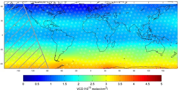
Fig. 1.Nadir VCDV∗for 28 January 2006. The marked area in the Pacific is the reference sector used in this study.
2.4 Stratospheric estimation schemes (SES)
The DOAS algorithm as described in Sect. 2.1 yields total SCDsSof NO2from the nadir measurements. The slant col-umn densitySis the concentration integrated along the effec-tive light path. It is usually converted into a vertical column density (VCD)V, i.e. the vertically integrated concentration, via the air mass factor (AMF)A:
V=S/A. (1)
The air mass factor has to be calculated by radiative trans-fer models and depends on observation geometry (SZA and Line-of-sight zenith angle LZA), ground albedo, aerosols, clouds, and the trace gas profile. The dominant dependen-cies are fundamentally different for stratospheric and tro-pospheric trace gases. For the considered nadir observa-tions with SZA below 80◦, stratospheric AMFs mainly de-pend on observation geometry and are thus well determined. Tropospheric AMFs, however, critically depend on ground albedo, clouds, aerosols, and the tropospheric trace gas pro-file, i.e. several parameters that have to be considered as ex-ternal input.
In this study, we focus on quantifying the effect of differ-ent stratospheric estimation schemes (SES) on tropospheric column densities. For this purpose, we defineV∗by apply-ing stratospheric AMFs to the total SCDs:
V∗:=S/AStrat, (2)
where stratospheric AMFsAStrat are calculated as function of SZA and LZA using the RTM McArtim (Deutschmann, 2009) for one representative stratospheric profile of NO2 with a concentration peak at 25 km. (If, instead, the ac-tual limb profiles would be used, the resulting stratospheric
AMFs deviate less than 0.3% for SZAs up to 70◦, and less than 1% for SZAs up to 80◦.)
The asterisk indicates that these VCDs cannot be inter-preted quantitatively as total VCDs, since the tropospheric fraction of the SCD was converted (inappropriately) with a stratospheric AMF. This has to be kept in mind for the inter-pretation of tropospheric residues and will be corrected be-low (2.5) by multiplication withAStrat, yielding tropospheric SCDs.
2.4.1 Reference sector method (RSM)
The basic idea of the simple RSM is that the stratospheric VCD at any place can be estimated by the total VCD over a remote region (typically the Pacific) of the same latitude. I.e. the RSM assumes that (1) a sufficiently clean reference sector (RS) with negligible tropospheric pollution can be de-fined, and (2) the global stratospheric VCD field does only depend on latitude3, but not on longitude8.
We follow this simple approach by defining a RS in the Pa-cific as indicated in Fig. 1, showingV∗for 28 January 2006 (additional examples for other days are shown in the Supple-ment). For every dayd, we calculate a look-up table (LUT) VRS∗ (d,3)by averaging the daily measurementsV∗over the RS in latitudinal bins of 1◦resolution.
A smoothed LUT VbRS∗ (d,3) is derived by convoluting VRS∗ (d,3)with Gaussian functions both in temporal (σ=5 days) and in latitudinal (σ=5◦) dimension. Both the non-smoothed (VRS∗(d,3)) and the smoothed LUTVbRS∗ (d,3)are shown in Fig. S1 of the Supplement.
Fig. 2. Stratospheric VCDLderived from integrated limb profiles 27–29 January 2006. Colour-coded disks indicate the location of the tangent points for the individual limb VCDsL, the map shows the interpolated and smoothed fieldL(d,3,φ)b .
For the RSM, we define the stratospheric VCDWRSM as function of daydand latitude3as:
WRSM(d,3):=VbRS∗ (d,3). (3) 2.4.2 Absolute limb correction (ALC)
Stratospheric limb VCDs (LVCDs)Lare calculated from the derived limb concentration profiles (see Sect. 2.2) by simply integrating the profiles from 15 km to 42 km. Varying the lower integration limit between 12 km and 18 km affects the resulting LVCDs by less then 5%. We therefore neglect the latitudinal variation of tropopause height in this study. Er-rors ofLare derived from integrating the uncertainties of the concentration in each layer as derived by the limb inversion. A LVCD error threshold of 0.25×10¹⁵molec/cm2is defined to eliminate outliers, which mainly occur due to the South Atlantic Anomaly, a depression in the Earths’ magnetic field (Van Allen belt).
Due to the co-adding of the four horizontal limb scans, one limb VCDLis available per limb state. On account of the alternating limb/nadir measurements, a single L could be used as (constant) stratospheric estimation for all mea-surements within the according nadir state, as in Sierk et al. (2006). However, in doing so, a single biasedLwould affect a complete nadir state. In addition, the assump-tion of a constant stratosphere within one nadir state leads to artificial step functions in the latitudinal dependency of the resulting TSCDs. Instead, we define a smoothed LUT b
L(d,3,8)by folding the limb VCDsLwith Gaussian func-tions G(σlon,σlat), where σlon=20◦×cos(3) and σlat= 10◦≈1000 km. These settings for σlon force smooth spa-tial patterns for low latitudes (σlon=20◦≈2000 km at the
equator), but allow for strong longitudinal gradients at higher latitudes (σlon=10◦≈500 km at 60◦latitude), which is par-ticularly necessary at the polar vortex.
To improve statistics and to avoid large spatial gaps, limb measurements of the previous and following day are included with half weight in the folding procedure. In addition, all limb CDs are weighted by the inverse square of their error.
Figure 2 shows a global map of limb VCDs on 28 Jan-uary 2006. The location of the limb tangent points of in-dividual LVCDs are marked by colour-coded disks, while the background map displays the smoothed LUTbL(d,3,8). Keep in mind that for the retrieval of the profile at the tangent point, all limb scans within the limb state, covering an area of about one thousand km extent both in latitudinal as in lon-gitudinal direction, are used for the inversion. The latitudinal dependency ofLselected over the RS on 28 January 2006 is added in Fig. 3 for an absolute comparison to the RS VCDs VRS∗ from nadir observations.
For the absolute limb correction scheme, we define the stratospheric VCD as
WALC(d,3,8):=bL(d,3,8). (4) 2.4.3 Relative limb correction (RLC)
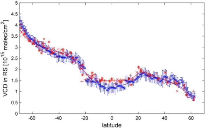
Fig. 3.Latitudinal dependencies ofVRS∗ (blue) andLRS(red). Nadir measurements are binned in 1◦bins and displayed as mean (*) and standard deviation (bar). Limb measurements are displayed for Jan-uary 27 (+), 28 (*), and 29 (x), 2006. The curves show the smoothed LUTsVbRS(d,3)(blue) andbLRS(d,3)(red).
Thus, we also perform arelativelimb correction, which by definition eliminates the deviations of limb and nadir VCDs in the RS. The basic idea is to apply the same RS correc-tion that was applied for the nadir VCDs also to the limb VCDs: from the limb VCDsLover the RS we derive a LUT b
LRS(d,3)by smoothing over time and latitude. The differ-ence ofLandbLRSat the same day and latitude holds infor-mation on longitudinal variations for a given latitude: 1L(d,3,8)=L(d,3,8)−bLRS(d,3). (5)
We denote 1L as Limb Longitudinal Variation (LLV). Figure 4 displays the individual 1L at the limb tangent points as disks, while the background map shows1Ldwhich is obtained by smoothing with the same settings asbL (see Sect. 2.4.2). Again, measurements of the previous and fol-lowing day are included with half weight.
Now we use the LLVd1Lto refine the classical RSM and define the stratospheric VCD from relative limb correction (RLC) as
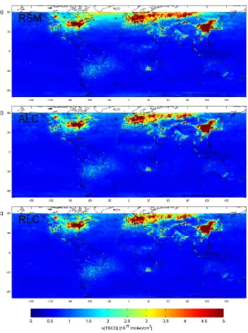
WRLC(d,3,8):=WRSM(d,3)+1L(d,3,8).d (6) Figure 5 compares global maps of stratospheric VCDsW for the three SES for 28 January 2006.
2.5 Tropospheric SCDs of NO2
With any of these estimatesW (i.e.WRSM,WRLC, orWALC) for stratospheric VCDs of NO2, we define the tropospheric residue as
1V∗:=V∗−W . (7) 1V∗ represents the tropospheric VCD derived with a stratospheric AMF. Due to the strong dependency of AStrat on observation geometry, 1V∗ strongly depends on
SZA and LZA, which is not realistic for tropospheric VCDs. To correct this inconsistency, we transfer1V∗back to a tro-posphericslantcolumn density (TSCD)T:
T:=1V∗×AStrat. (8)
FromT, a tropospheric VCD can be derived directly by applying the appropriate tropospheric AMF (and a tempera-ture correction to account for the “cold” NO2cross-section at 220 K used in the DOAS-fit, see Sect. 2.2). Within this study, however, we do not apply tropospheric AMFs, since we want to focus solely on the effect of different SES, with-out involving (and discussing the impact of) external datasets (for ground albedo, clouds/aerosols and profiles). For orien-tation, however, note that tropospheric AMFs for cloud free scenes are of the order of 1 (Richter and Burrows, 2002), and generally<1 for clouded scenes, except for cases with substantial NO2within/above the cloud.
All total CDs (V∗) and all stratospheric CDs (W) pre-sented in this study are vertical column densities, whereas the tropospheric CDs T discussed below are slant column densities. This differentiation is potentially confusing, but necessary, since stratospheric CDs need to be processed in terms of VCDs (e.g. for the averaging of RS column den-sities of the same latitude for different SZA/LZA), but the relevant tropospheric CDs, prior to the application of tropo-spheric AMFs, are slant column densities. Thus, we discuss the effect of the different SES on tropospheric CDs in terms of SCDs in Sects. 3 and 4. The stratospheric AMF, i.e. the ratio ofT and1V∗, is slightly above 2 for low SZA (tropics) up to 7 for high SZA (80◦).
The resulting TSCDs for the three different SES are dis-played in Fig. 6.
2.6 Intrinsic error information
In this section we briefly discuss the potential of detecting and estimating systematic as well as statistical errors from the measurements themselves. A more detailed discussion of this issue and the actual definition of the terms we use for quantitative error information are given in Sect. S3 of the Supplement.
Fig. 4.Longitudinal Limb Variation (LLV)1Lfor 28 January 2006. Disks show the LLV for the individual limb states (1L), the map shows the interpolated and smoothed fieldd1L(d,3,8).
Additional information on both statistical and systematic errors can be derived from the standard deviation (over lon-gitude) of W in the reference sector. This quantity com-prises statistical errors (e.g. from the DOAS fit error and nat-ural fluctuations of stratospheric VCDs), but enhanced val-ues clearly indicate additional systematic errors, e.g. due to fit artefacts over oligotrophic oceanic regions.
From the comparison of individual LLV 1L to the smoothed LUT1L, information on the performance of thed smoothing/interpolation procedure can be derived, mainly in cases of strong temporal and spatial gradients.
In Sect. S3 of the Supplement, we define and display the error quantitiesδWRSMandδWRLC, which are automatically calculated during the TSCD retrieval, and are provided as function of day and latitude. Thus, although shortcomings of the RLC remain for some regions and times, these can be recognized by enhanced values ofδWRSMorδWRLC.
3 Results
In this section, we present TSCDs for the different SES, and analyze their specific characteristics and differences. Again, we focus on wintertime, where the shortcomings of the RSM become particularly evident. Results for other times of the year are presented in the Supplement and also shortly dis-cussed below.
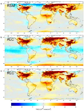
Figure 6 exemplarily shows the resulting TSCDs TRSM, TALC, and TRLC for 28 January 2006. Note that the col-orscale has been chosen to accentuate small systematic de-viations from 0 – in particular negative ones – over “clean” regions. Polluted regions like Europe, the east coast of the United States, or China, are by far in saturation.
As can be seen in Fig. 4, the simple assumption of a zonally constant stratospheric CD is not valid. As a consequence, the RSM leads to – unphysical – negative TSCDsTRSM (Fig. 6a) over the Northern Atlantic down to −2×10¹⁵molec/cm2, which is far below the statistical un-certainty. In contrast,TRSMover wide areas in remote North-ern Asia is quite high. Similar shortcomings of the RSM in wintertime have been discussed in, e.g. Richter and Bur-rows (2002) or Sierk et al. (2006).
The ALC (Fig. 6b) significantly improves the patterns over the Northern Atlantic, and the strong negative bias is successfully corrected. However, TALC shows strong lati-tudinal features, both positive and negative: oceanic CDs around the equator are negative now (in contrast to TRSM) about−1×10¹⁵molec/cm2, andT
ALCis unrealistically high (2×10¹⁵molec/cm2) south of 60◦S, i.e. far from any known source of NOx. This is a direct consequence of the differ-ent latitudinal dependencies ofVRS∗ andLRS(Fig. 3), which reveals systematic deviations that lead to negative (20◦S to 20◦N) as well as positive (south of 60◦S) background TSCDsTALC. Keep in mind that Fig. 3 displays VCDs; the differences in TSCD (Fig. 6b) are higher by the stratospheric AMFAStrat, which varies from about 2 in the tropics up to 7 at high latitudes.
Fig. 5.Stratospheric VCDsWon 28 January 2006 for the different stratospheric estimation schemes:(a)reference sector method,(b)
absolute limb correction, and(c)relative limb correction.
The longitudinal variations in TRSM at about 60◦S are reduced in TRLC, but could not be removed completely by the RLC. Generally, patterns at Northern hemispheric (NH) mid– and high latitudes are corrected successfully by the RLC, but are only lessened in the Southern Hemisphere (SH), as illustrated by the additional examples given in the Supplement, and discussed in Sect. 4.
After illustrating the different TSCDs for a specific day, we compare monthly climatologies (mean 2003–2008) of TSCDs for January (Fig. 7) and additional months in the Sup-plement (Figs. S11–S16). Obviously, the longitudinal varia-tions of stratospheric NO2, as observed for 28 January 2006, do not cancel out by temporal averaging, but instead system-atic spatial patterns stand out.
Mean JanuaryTRSM (Fig. 7) is negative down to −2× 10¹⁵molec/cm2over large parts of Canada and the Northern Atlantic, and quite high (>1×10¹⁵molec/cm2) throughout northeastern Russia. Like for the single day sample (Fig. 6), the ALC reduces/removes these longitudinal variations, but introduces zonal stripes of negative TSCDs around the equa-tor, and high positive TSCDs south of 60◦S (Fig. 7b). Again, TRLCimproves the longitudinal variations while retaining the RS levels to 0 on average (Fig. 7c).
Fig. 6. Tropospheric SCDs for 28 January 2006.(a)TRSM: refer-ence sector method.(b)TALC: absolute limb correction.(c)TRLC: relative limb correction. Crosses mark the locations considered in the time-series analysis (see Figs. 11–12).
The differences of the mean TSCDs are shown in Fig. 8, directly illustrating the effects of the different stratospheric estimation schemes. Compared to RSM, both ALC (Fig. 8a) and RLC (Fig. 8b) remove a dipolar pattern with a max-imum amplitude of 2.5×10¹⁵molec/cm2 at northern lati-tudes. However, the ALC introduces zonal stripes in the cli-matology up to 1.2×10¹⁵molec/cm2over the RS at the equa-tor (Fig. 8a and c). In contrast, the differenceTRSM−TRLCis negligible for latitudes between 30◦N and 60◦S.
Fig. 7.Mean tropospheric SCDs for January 2003–2008.(a)TRSM: reference sector method. (b)TALC: absolute limb correction. (c) TRLC: relative limb correction.
Aside from the effect of the different SES on mean val-ues, we also analyzed the standard deviationss of TSCDs over time for January 2003–2008 (Fig. 9). As expected, standard deviations are generally high over polluted re-gions, where mean TSCDs are enhanced, due to variabil-ity of tropospheric CDs. Beyond that, s(TRSM) is high (>3×10¹⁵molec/cm2) over the Northern Atlantic, in con-trast tos(TALC)ands(TRLC). Figure 10, which shows the differences of standard deviations, reveals that bothTALCand TRLC lead to lower standard deviations over large areas at high latitudes. The consideration of longitudinal variations from limb measurements thus clearly reduces the standard deviations by about 1 up to 3×10¹⁵molec/cm2 compared to the simple RSM. Note that standard deviations of TALC andTRLCare almost identical (Fig. 10c), despite their differ-ences in mean values. This indicates thats(TALC)is driven by tropospheric variability and stratospheric dynamics, but notby the zonal stripes introduced by the ALC, which are thus rather constant in magnitude and location for a fixed month.
Figures S4–S16 of the Supplement illustrate that the RLC also improves the spatial patterns, both on individual days as well as in monthly climatologies, for other times of the year. Typical values for daily LLVs (in terms of VCD) are below
Fig. 8. Difference of mean tropospheric SCDsTRSM−TALC(a), TRSM−TRLC(b), andTRLC−TALC(c)for January 2003–2008.
±0.3×10¹⁵molec/cm2for low latitudes, but can reach±0.6 up to 1×10¹⁵molec/cm2for higher latitudes in some months (Figs. S4, S6, S8). Figure S10 illustrates that the principal shortcoming of the ALC, caused by different latitudinal de-pendencies ofV∗andL, withLbeing generally higher than V∗, is present throughout the year.
For the monthly climatologies, the RLC modifies the re-sulting TSCDs by less than 0.5×10¹⁵molec/cm2for low and midlatitudes, and up to 1×10¹⁵molec/cm2 at high north-ern latitudes (about 60◦) in April and October. In October, the differenceTRSM−TRLC is up to 3×10¹⁵molec/cm2 at 60◦S, and still unrealistic spatial patterns (negativeTRLC) are present (Figs. S15–S16). Thus, especially for the SH, the RLC sometimes reduces, rather than completely elimi-nates the artefacts of the RSM. Nevertheless, standard devi-ations ofTRSMare always significantly reduced by the RLC (Figs. S12, S14, S16).
Fig. 9.Standard deviations of tropospheric SCDs for January 2003– 2008.(a)s(TRSM),(b)s(TALC),(c)s(TRLC).
Figure 11 shows the annual cycles of the different TSCDs. Figure 12 displays the respective frequency distributions and lists means and standard deviations for these four locations.
The first location (20◦W, 50◦N) is located in the Northern Atlantic.TRSM(blue) is often negative and generally show a high variability in winter. This variability is reduced both in TALC(green) andTRLC(orange). However,TALCshows sys-tematically higher CDs in summer. While the mean ofTRSM is negative,TRLC is almost zero on average. The standard deviations both ofTALCandTRLCare reduced compared to TRSM.
At the second location, placed in Russia (110◦E, 50◦N) far from large cities, wintertimeTRSM is quite high (up to 5×10¹⁵). On average,T
RSMis 0.67×10¹⁵molec/cm2. ALC reduces these high wintertime TSCDs, but introduces too high TSCDs in summertime. TRLC is close to zero on av-erage and has a reduced standard deviation.
The SH locations, (20◦W and 110◦E, 50◦S) are over Ocean, far from known NOxsources. The annual cycle and frequency distributions of both southern locations are simi-lar:TRSMshows high variability and high CDs in SH winter (NH summer). ALC overcorrects the SH wintertime TSCDs, resulting in negative TALC down to −5×10¹⁵molec/cm2. Again,TRLC is close to zero on average and has a reduced standard deviation.
Fig. 10.Difference of the standard deviations of tropospheric SCDs s(TRSM)−s(TALC)(a), s(TRSM)−s(TRLC)(b), and s(TRLC)− s(TALC)(c)for January 2003–2008.
For all considered clean locations, the mean of TRLC is non-negative, close to zero, and its standard deviation is low-est, indicating that RLC is the most realistic SES.
4 Discussion
Estimating the stratospheric column density over a remote reference sector is an easy, robust method for the retrieval of tropospheric CDs, and has been used successfully in sev-eral studies on tropospheric NO2. In particular, it implies a first-order correction of any systematic offset in total CDs. The simple assumption of zonal constancy, however, clearly fails at higher latitudes, in particular close to the polar vortex. We present two advanced stratospheric estimation schemes (ALC and RLC) involving additional limb measurements and apply them to 6 years of SCIAMACHY measurements.
Fig. 11.Annual cycle of TSCDs for four selected locations (as marked in Figs. 6–10). Upper row: 50◦N. Lower row: 50◦S. Left column: 20◦W. Right column: 110◦E. The different schemes are marked by colors: blue (TRSM), green (TALC), and orange (TRLC).
Stratospheric correction by ALC generally improves spa-tial patterns of TSCDs compared to the RSM with respect to longitudinal variations. However, in the resulting TSCDs TALC, systematic zonal stripes (about±1×10¹⁵molec/cm2 in monthly climatologies) show up as a consequence of dif-ferent latitudinal dependencies ofVRS∗ andLRS. Generally, LishigherthanV∗ for low/mid latitudes most time of the year, resulting in negativeTALC. Low or even negative tropo-spheric CDs, resulting from subtraction of stratotropo-spheric limb VCDs, can also be seen in Sioris et al. (2004) (Fig. 6 therein) and in PROMOTE (2004).
The following aspects might lead to systematic biases in nadir and/or limb data, thus potentially causing different lat-itudinal dependencies:
– The DOAS retrievals for nadir and limb use different cross-sections for NO2 (see Sects. 2.2 and 2.3). As a consequence, limb CDs are systematically higher (com-pared to a fit using the NO2cross-section from Vandaele et al., 1998) by about 4%. In addition, total nadir SCDs might be biased due to artificial spectral structures in the direct solar reference measurement, caused by the optical system (diffusor plate). However, the observed zonal stripes can not be eliminated, neither by re-scaling nor by simply adding a constant offset to total SCDs.
– In our analysis, we define the limb VCDLas the in-tegrated limb concentration from 15 km to 42 km. We thereby neglect latitudinal variations of the tropopause height (TH), and thus generally tend to overestimateL over the tropics, and underestimate it at high latitude. We investigated the impact of the TH onLby varying it between 12 and 18 km. The resulting modifications of L are below 5%, corresponding to absolute values of 0.05 to 0.25×10¹⁵molec/cm2. For an absolute limb correction scheme, the fixed TH can thus lead to signif-icant errors in the limb estimation, in particular for high latitudes. However, our choice of a fixed TH can not explain the different latitudinal dependencies of ofV∗ andL seen in Fig. 2 and Fig. S10 of the Supplement, and the resulting zonal bands inTALC.
– Although limb and nadir measurements are performed from the same platform, there is a time shift of about 7 minutes between the limb- and the nadir sounding of the stratosphere. For high SZA (sunrise and sunset), this may be long enough for significant differences of NO2 due to changes in photochemistry.
Fig. 12.Frequency distribution of TSCDs for four selected locations (as marked in Figs. 6–10). Upper row: 50◦N. Lower row: 50◦S. Left column: 20◦W. Right column: 110◦E. The different schemes are marked by colors: blue (TRSM), green (TALC), and orange (TRLC). The numbers give the respective means and standard deviations (in 1015molec/cm2).
(e.g. over the ITCZ) results in an underestimation of box AMFs in and above the clouds. However, the to-tal limb column would only be affected significantly, if there would be high NO2 concentrations in/directly above the cloud.
– Clouds potentially affect the nadir total SCDs by their impact on the Earth shine spectra, e.g. via their impact on polarization, the probability of inelastic scattering (Ring effect), or the shielding of light reflected at the ground, carrying spectral albedo information. The latter could be important especially over the problematic olig-otrophic oceanic regions. Yet, we find no correlation of TSCDs and cloud fraction (R= −0.01 for 28 Jan-uary 2006, over the RS).
– In addition, clouds lead to increased stratospheric AMFs, which is only a small effect (<2% difference betweenAStratfor cloud-free versus clouded conditions, as calculated with McArtim), and thus not considered in this study.
– The limb inversion scheme is based on one dimensional RTM, assuming horizontal homogeneity. In cases of horizontal gradients, this simplification leads to errors in the resulting profiles, since the effective light paths
for low tangent heights do not reach as close to the tan-gent point as for high tantan-gent heights. At the Arctic polar vortex, the corresponding errors for NO2 concen-trations were found to be 20% on average (Puk¸¯ıte et al., 2008). Currently, 3-D effects are investigated and quan-tified for the SH polar vortex, as well as for midlatitudes and tropics, where substantial latitudinal gradients can also occur (Puk¸¯ıte et al., 2010). This study uses mea-surements of successive orbits in exclusive limb geom-etry in December 2008, following the SCIAMACHY operation change request OCR #38). Total errors of in-tegrated VCDs are of the order of 0.1×10¹⁵molec/cm2 for strong horizontal gradients. But though the simpli-fication of a 1-D retrieval results in systematic errors, those can not explain the particular differences in the latitudinal dependencies ofV∗andL.
shortcomings of the nadir and/or limb retrievals in future studies. But at present, as shown in this study, the direct ALC is not appropriate for an automatized retrieval of NO2 TSCDs.
A third method, the RLC, was quite successful in re-moving longitudinal variations without the drawbacks of the ALC. By applying the RSM to nadir and limb data alike, an absolute calibration of vertical column densities (limb and nadir) is not required, and systematic biases are first-order corrected. Also possible jumps in the time series (due to, e.g. calibration setting changes) and degradation effects are automatically corrected for. The RLC thus keeps the her-itage of the RSM, i.e. being a simple, robust, and model-independent correction scheme, but clearly improves spatial patterns of the resulting TSCDs, where longitudinal varia-tion causes the RSM to fail. Over clean regions, meanTRLC is generally close to 0, and its standard deviation is the lowest of all SES. The RLC introduces changes in TSCD (compared to RSM) up to 3×10¹⁵molec/cm2for some months (January, Fig. 8b; October, Fig. S16a in the Supplement), while in NH summer, changes are generally low (<0.5×10¹⁵molec/cm2 for July, Fig. S14a in the Supplement).
Although the RLC is a significant improvement over the simple RSM, it is not capable of eliminating stratospheric features completely. In particular for the SH, spatial patterns that are obviously not of tropospheric origin remain in maps of TRLC. Possible reasons for these pronounced SH short-comings are:
– Especially in the SH, very localized stratospheric fea-tures occur. For instance, on 24 October 2005, a small filament of enhanced NO2CDs is visible in the map of V∗south of Africa (see Figs. S8 and S9 of the Supple-ment) . Limb VCDsLfor this region are also enhanced, i.e. the observed NO2is located in the stratosphere. Al-though the limb measurements are capable of detecting this feature, they can not fully resolve the spatial struc-ture of this filament due to their coarse spatial resolu-tion (one profile per state). This inevitably leads to an incomplete correction of this structure by the RLC (see Fig. S9c). This shortcoming is reflected by a high value forδWRLC(and thusδTRLC), which regularly occurs in autumn at 60◦S (Fig. S3).
– As discussed above, the neglection of 3-D effects results in systematic errors: at the Arctic polar vortex (where the concentration gradient is positive in viewing direc-tion), concentrations (and thus integrated VCDs) are un-derestimated, and, vice versa, at the Antarctic polar vor-tex, VCDs are overestimated. Thus, in particular for the SH, longitudinal variations should rather be overcom-pensated by applying the LLV. Hence, 3-D effects can not explain the insufficient correction for the SH.
– Limb measurements are performed in forward direction, i.e. southwards for the descending orbits. I.e. at high northern latitudes, limb measurements “look” from high to low SZA, with the sun ahead, and vice versa at high southern latitudes. This is a systematic difference of the observation geometries of both hemispheres which may at least partly explain why the RLC is less successful in the SH.
One remaining possible shortcoming of both RSM and RLC are systematic biases of total nadir SCDs due to spectral interference of water absorption and vibrational Raman scat-tering. This potentially affects the stratospheric estimation around 30◦S, with impact on tropospheric CDs over southern South America, South Africa, and Australia. From the spa-tial variations of NO2in and outside oligotrophic oceanic re-gions, we estimate this bias to be below 0.5×10¹⁵molec/cm2 (in terms of TSCDs). Further improvements of the spectral fit are the purpose of ongoing studies.
While the ALC should, principally, yield “total” tropo-spheric CDs, the TSCDs from RSM and RLC are, by def-inition, troposphericexcessCDs w.r.t. the reference sector: the small, but existent tropospheric NO2 SCDs are inter-preted as stratospheric SCD. For quantitative interpretation of TRSM andTRLC, modelled TSCDs in the RS have to be added, which are of the order of 0.3–0.6×10¹⁵molec/cm2, depending on latitude (Martin et al., 2002). Alternatively, for comparisons ofTRLC(“pure” measurement) to modelled TSCDs, the same RS correction could be applied to the latter (Franke et al., 2009).
The changes in TSCDs between the different SES are sig-nificant, and have a strong impact on quantitative studies of tropospheric NO2, like emission estimates. In particular over Siberia, RLC leads to TSCDs that are lower compared to TRSM by about 1 to 2×10¹⁵molec/cm2 in a climatol-ogy for January 2003–2008. Over Europe, on the other hand,TRLCis higher thanTRSMby about 1×10¹⁵molec/cm2. Over polluted European sites, mean wintertime TSCDs reach values of about 4×10¹⁵molec/cm2 (Paris) up to >10× 1015molec/cm2(Milan) (on a 0.5◦×0.5◦grid), i.e. the RLC SES has significant impact on TSCDs even at polluted sites. For hemispheric spring and summer, effects are generally smaller, but still systematic differences of RSM and RLC of the order of 0.2–0.4×10¹⁵molec/cm2occur over large areas. Though the RSM is an established SES, our study em-phasizes the need to account for longitudinal variations of stratospheric NO2. This also affects studies on relative sig-nals (e.g. the Sunday reduction of the weekly cycle), as the RSM bias is additive, not multiplicative (see Eq. 7). In stud-ies on NO2in remote regions at high latitudes with relatively low TSCD levels, e.g. soil emission estimates over deserted regions like Siberia, the impact of the stratospheric estima-tion and the related uncertainties have to be kept in mind.
5 Conclusions
In this study, we analyzed different schemes for the estima-tion of stratospheric column densities (CDs) of NO2, involv-ing limb measurements from the SCIAMACHY instrument, and the consequences for the resulting tropospheric CDs.
Estimating the stratospheric CDs by a simple reference sector method (RSM), which is generally a robust and successful method, leads to systematic errors in strato-spheric CDs. Consequently, tropospheric CDs are nega-tive over the Atlantic (50◦N) down to −4×10¹⁵ (daily extreme)/−1×1015molec/cm2(monthly climatology) in au-tumn/winter months.
A direct, absolute limb correction (ALC) is capable of cor-recting longitudinal variations of stratospheric CDs, thus be-ing an improvement compared to the simple reference sector method at high latitudes. However, the latitudinal dependen-cies of limb and nadir CDs turned out to be systematically different. Further validation of nadir CDs and limb profiles, especially at low latitudes, is needed, to investigate and even-tually understand these different latitudinal dependencies, which let an automatized retrieval of tropospheric CDs by the ALC fail.
Instead, we developed a relative limb correction (RLC) scheme which successfully improves the RSM w.r.t. longitu-dinal features, without introducing artefacts elsewhere, and suggest using this scheme for the retrieval of tropospheric NO2CDs. The RLC keeps the heritage of the simple RSM, i.e. it is based on measurements and free of a-priori assump-tions (like NOx emissions or modelled stratospheric CDs),
but significantly improves the shortcomings of the RSM. Compared to both RSM and ALS, the spatial patterns of the CDs derived by RLC are the most plausible, i.e. means are closest to zero for clean regions and standard deviations over time are the lowest.
Although the RLC generally works successfully, spatial features of stratospheric origin partly remain in tropospheric CDs, especially for high southern latitudes. Fortunately, re-gions south of 50◦S are not in the focus of studies on tropo-spheric NO2. Nevertheless, it is of course desirable to over-come the remaining shortcomings by future improvements.
Error quantities are defined as a function of day and lat-itude, considering (a) the standard deviation of CDs in the RS and (b) deviations of smoothed and non-smoothed strato-spheric maps. These quantities provide information on both statistical and especially systematic errors, like shortcomings of the DOAS fit over oligotrophic oceans, or scenarios with high spatial gradients of stratospheric NO2which are not re-solved by the limb measurements.
The RLC was discussed for NO2in this study. In princi-ple, it could also be applied to other trace gases like O3. For such an adaptation, the specific characteristics of the differ-ent trace gas retrievals and the specific spatial patterns (pro-files as well as global distribution) have to be considered in detail. In particular for BrO, the method will be proba-bly insufficient, since the regions of interest for BrO are po-lar, i.e. solar zenith angles are high, and stratospheric BrO profiles are too low to be fully captured by the limb measure-ments.
The available dataset on limb longitudinal variations can be used to check and improve other stratospheric estimation algorithms, in particular advanced RS methods working with 2-D interpolation or wave fitting. This is important for cur-rent and future satellite spectrometers without the limb view-ing mode. Furthermore, the information on the longitudinal dependency of stratospheric NO2CDs, as provided by SCIA-MACHY limb measurements, might also be used to improve RSM stratospheric estimations for other satellite instruments, like OMI or GOME-2. However, for such applications, dif-ferences in local times of the measurements have to be con-sidered.
Acknowledgements. We thank ESA and DLR for providing SCIAMACHY spectra. Sven K¨uhl is funded by the DFG (Deutsche Forschungsgemeinschaft). We gratefully acknowledge valuable discussions with Andreas Richter and Andreas Hilboll. We thank Folkert Boersma, Howard K. Roscoe and two anonymous reviewers for helpful comments. We are grateful to Marloes Pen-ning de Vries for fruitful scientific discussions and editorial support.
The service charges for this open access publication have been covered by the Max Planck Society.
References
Beirle, S., Platt, U., Wenig, M., and Wagner, T.: Weekly cycle of NO2by GOME measurements: a signature of anthropogenic sources, Atmos. Chem. Phys., 3, 2225–2232, 2003,
http://www.atmos-chem-phys.net/3/2225/2003/.
Beirle, S.: Estimating source strengths and lifetime of Nitrogen Ox-ides from satellite data, Ph.D. Thesis, University of Heidelberg, 2004.
Boersma, K. F., Eskes, H. J., and Brinksma, E. J.: Error analysis for tropospheric NO2 retrieval from space, J. Geophys. Res., 109, D04311, doi:10.1029/2003JD003962, 2004.
Boersma, K. F., Eskes, H. J., Veefkind, J. P., Brinksma, E. J., van der A, R. J., Sneep, M., van den Oord, G. H. J., Levelt, P. F., Stammes, P., Gleason, J. F., and Bucsela, E. J.: Near-real time retrieval of tropospheric NO2from OMI, Atmos. Chem. Phys., 7, 2103–2118, 2007,
http://www.atmos-chem-phys.net/7/2103/2007/.
Bogumil, K., Orphal, J., Homann, T., Voigt, S., Spietz, P., Fleis-chmann, O. C., Vogel, A., Hartmann, M., Bovensmann, H., Fr-erick, J., and Burrows, J. P.: Measurements of molecular absorp-tion spectra with the SCIAMACHY pre-flight model: Instrument characterization and reference data for atmospheric remote sens-ing in the 230–2380 nm region, J. Photochem. Photobiol. A., 157, 167–184, 2003.
Bovensmann, H., Burrows, J. P., Buchwitz, M., Frerick, J., No¨el, S., Rozanov, V. V., Chance, K. V., and Goede, A. P. H.: SCIA-MACHY: Mission objectives and measurement modes, J. Atmos. Sci., 56(2), 127–150, 1999.
Br¨uhl, C. and Crutzen, P. J.: MPIC two-dimensional model, in: The Atmospheric Effect of Stratospheric Aircraft, 1292, edited by: Prather, M. J. and Remsberg, E. E., NASA Ref. Publications, 103–104, 1993.
Bucsela, E. J., Celarier, E. A., Wenig, M. O., Gleason, J. F., Veefkind, J. P., Boersma, K. F., and Brinksma, E. J.: Algorithm for NO2Vertical Column Retrieval from the Ozone Monitoring Instrument, IEEE T. Geosci. Remote, 44(5), 1245–1258, 2006. Burrows, J., Weber, M., Buchwitz, M., Rozanov, V. V.,
Ladst¨adter-Weissenmayer, A., Richter, A., de Beek, R., Hoogen, R., Bram-stedt, K., Eichmann, K.-U., Eisinger, M., and Perner, D.: The Global Ozone Monitoring Experiment (GOME): Mission con-cept and first scientific results, J. Atmos. Sci., 56, 151–175, 1999. Butz, A., B¨osch, H., Camy-Peyret, C., Chipperfield, M., Dorf, M., Dufour, G., Grunow, K., Jeseck, P., K¨uhl, S., Payan, S., Pepin, I., Pukite, J., Rozanov, A., von Savigny, C., Sioris, C., Wagner, T., Weidner, F., and Pfeilsticker, K.: Inter-comparison of strato-spheric O3and NO2abundances retrieved from balloon borne di-rect sun observations and Envisat/SCIAMACHY limb measure-ments, Atmos. Chem. Phys., 6, 1293–1314, 2006,
http://www.atmos-chem-phys.net/6/1293/2006/.
Deutschmann, T.: Atmospheric radiative transfer modelling using Monte Carlo methods, Diploma Thesis, Universit¨at Heidelberg, 2009.
Dorf, M., B¨osch, H., Butz, A., Camy-Peyret, C., Chipperfield, M. P., Engel, A., Goutail, F., Grunow, K., Hendrick, F., Hrechanyy, S., Naujokat, B., Pommereau, J.-P., Van Roozendael, M., Sioris, C., Stroh, F., Weidner, F., and Pfeilsticker, K.: Balloon-borne stratospheric BrO measurements: comparison with En-visat/SCIAMACHY BrO limb profiles, Atmos. Chem. Phys., 6, 2483–2501, 2006,
http://www.atmos-chem-phys.net/6/2483/2006/.
Fishman, J. and Balok, A. E.: Calculation of daily tropospheric ozone residuals using TOMS and empirically improved SBUV measurements: Application to an ozone pollution episode over the eastern United States, J. Geophys. Res.-Atmos., 104, 30319– 30340, 1999.
Franke, K., Richter, A., Bovensmann, H., Eyring, V., J¨ockel, P., Hoor, P., and Burrows, J. P.: Ship emitted NO2 in the Indian Ocean: comparison of model results with satellite data, Atmos. Chem. Phys., 9, 7289–7301, 2009,
http://www.atmos-chem-phys.net/9/7289/2009/.
Heckel, A., Richter, A., Rozanov, A., and Burrows, J. P.: Limb Nadir Matching: Retrieval of tropospheric NO2 columns using SCIAMACHY Nadir and Limb mea-surements, Presentation at the workshop “Tropospheric NO2 measured by satellites”, 10–12 September 2007, KNMI, De Bilt, The Netherlands, online available at: http://www.knmi.nl/research/climate observations/events/ no2 workshop/presentations/Presentations/107 Heckel.ppt, last access: February 2010, 2007.
K¨uhl, S., Puk¸¯ıte, J., Deutschmann, T., Platt, U., and Wagner, T.: SCIAMACHY Limb Measurements of NO2, BrO and OClO, Re-trieval of vertical profiles: Algorithm, first results, sensitivity and comparison studies, Adv. Space Res., 42, 1747–1764, 2008. Leue, C., Wenig, M., Wagner, T., Klimm, O., Platt, U., and J¨ahne,
B.: Quantitative analysis of NOxEmissions from Global Ozone Monitoring Experiment satellite image sequences, J. Geophys. Res., 106, 5493–5505, 2001.
Levelt, P. F., van den Oord, G. H. J., Dobber, M. R., Malkki, A., Visser, H., de Vries, J., Stammes, P., Lundell, J. O. V., and Saari, H.: The ozone monitoring instrument, IEEE T. Geosci. Remote, 44(5), 1093–1101, 2006.
Martin, R. V., Chance, K., Jacob, D. J., Kurosu, T. P., Spurr, R. J. D., Bucsela, E., Gleason, J. F., Palmer, P. I., Bey, I., Fiore, A. M., Li, Q., Yantosca, R. M., and Koelemeijer, R. B. A.: An improved retrieval of tropospheric nitrogen dioxide from GOME, J. Geophys. Res., 107(D20), 4437, doi:10.1029/2001JD001027, 2002.
Martin, R. V.: Satellite remote sensing of surface air quality, Atmos. Environ., 42, 7823–7843, 2008.
Menke, W.: Geophysical data analysis: discrete inverse theory, Academic Press, 1999.
Platt, U. and Stutz, J., Differential Optical Absorption Spectroscopy Principles and Applications, Series: Physics of Earth and Space Environments, Springer, ISBN 978-3-540-21193-8, 2008. Polovina, J. J., Howell, E. A., and Abecassis, M.: Oceans least
pro-ductive waters are expanding, Geophys. Res. Lett., 35, L03618, doi:10.1029/2007GL031745, 2008.
PROMOTE, PROtocol MOniToring for the GMES Service Element on Atmospheric Composition, online available at: http://www. iup.uni-bremen.de/doas/no2 promote.htm, last access: February 2010, 2004.
Puk¸¯ıte, J., K¨uhl, S., Deutschmann, T., Platt, U., and Wagner, T.: Ac-counting for the effect of horizontal gradients in limb measure-ments of scattered sunlight, Atmos. Chem. Phys., 8, 3045–3060, 2008,
http://www.atmos-chem-phys.net/8/3045/2008/.
Puk¸¯ıte, J., K¨uhl, S., Deutschmann, T., Platt, U., and Wagner, T.: Extending differential optical absorption spectroscopy for limb measurements in the UV, Atmos. Meas. Tech. Discuss., 2, 2919– 2982, 2009,
http://www.atmos-meas-tech-discuss.net/2/2919/2009/. Puk¸¯ıte, S. K¨uhl, T. Deutschmann, U. Platt, and Wagner, T.: Profile
retrieval from SCIAMACHY limb measurements by global 2-D tomography, in preparation, 2010.
Richter, A. and Wagner, T.: Diffuser Plate Spectral Structures and their Influence on GOME Slant column densities, Techni-cal Note, online available at: http://joseba.mpch-mainz.mpg.de/ pdf dateien/diffuser gome.pdf, last access: February 2010, Jan-uary 2001, 2001.
Richter, A. and Burrows, J. P.: Tropospheric NO2 from GOME Measurements, Adv. Space Res., 29(11), 1673–1683, 2002. Richter, A., Burrows, J. P., N¨uß, H., Granier, C., and Niemeier, U.:
Increase in tropospheric nitrogen dioxide over China observed from space, Nature, 437, 129–132, doi:10.1038/nature04092, 2005.
Sierk, B., Richter, A., Rozanov, A., von Savigny, Ch., Schmolt-ner, A. M., Buchwitz, M., Bovensmann, H., and Burrows, J. P.: Retrieval and monitoring of atmospheric trace gas con-centrations in nadir and limb geometry using the space-borne SCIAMACHY instrument, Environ. Monit. Assess., 120, 65–77, doi:10.1007/s10661-005-9049-9, 2006.
Sioris, C. E., Kurosu, T. P., Martin, R. V., and Chance, K.: Strato-spheric and tropoStrato-spheric NO2 observed by SCIAMACHY: first results Adv. Space Res., 34(4), 780–785, 2004.
Vandaele, A. C., Hermans, C., Simon, P. C., Carleer, M., Col-ins, R., Fally, S., M´erienne, M. F., Jenouvrier, A., and Co-quart, B.: Measurements of the NO2absorption cross-sections from 42 000 cm−1to 10 000 cm−1(238–1000 nm) at 220 K and 294 K, J. Quant. Spectrosc. Radiat. Transfer, 59, 171–184, 1998. Vasilkov, A. P., Joiner, J., Gleason, J., and Bhartia, P.: Ocean Raman scattering in satellite backscatter UV measurements, Geophys. Res. Lett., 29, 1837–1840, 2002.
Vountas, M., Richter, A., Wittrock, F., and Burrows, J. P.: Inelastic scattering in ocean water and its impact on trace gas retrievals from satellite data, Atmos. Chem. Phys., 3, 1365–1375, 2003, http://www.atmos-chem-phys.net/3/1365/2003/.
Wagner, T., Beirle, S., Deutschmann, T., Eigemeier, E., Franken-berg, C., Grzegorski, M., Liu, C., Marbach, T., Platt, U., and Penning de Vries, M.: Monitoring of atmospheric trace gases, clouds, aerosols and surface properties from UV/vis/NIR satellite instruments, J. Opt. A., Pure Appl. Opt., 10, 104019, doi:10.1088/1464-4258/10/10/104019, 2008.
Wenig, M., K¨uhl, S., Beirle, S., Bucsela, E., J¨ahne, B., Platt, U., Gleason, J., and Wagner, T.: Retrieval and analysis of strato-spheric NO2 from the Global Ozone Monitoring Experiment, J. Geophys. Res., 109, D04315, doi:10.1029/2003JD003652., 2004.