www.atmos-chem-phys.net/14/8813/2014/ doi:10.5194/acp-14-8813-2014
© Author(s) 2014. CC Attribution 3.0 License.
Sources and geographical origins of fine aerosols in Paris (France)
M. Bressi1,2, J. Sciare1, V. Ghersi3, N. Mihalopoulos4, J.-E. Petit1,5, J. B. Nicolas1,2, S. Moukhtar3, A. Rosso3, A. Féron1, N. Bonnaire1, E. Poulakis4, and C. Theodosi4
1Laboratoire des Sciences du Climat et de l’Environnement, LSCE, UMR8212, CNRS-CEA-UVSQ, Gif-sur-Yvette, 91191, France
2French Environment and Energy Management Agency, ADEME, 20 avenue du Grésillé, BP90406 49004, Angers CEDEX 01, France
3AIRPARIF, Surveillance de la Qualité de l’Air en Ile-de-France, Paris, 75004, France 4Environmental Chemical Processes Laboratory (ECPL) Heraklion, Voutes, Greece
5INERIS, DRC/CARA/CIME, Parc Technologique Alata, BP2, Verneuil-en-Halatte, 60550, France Correspondence to: M. Bressi (michael.bressi@ensiacet.fr)
Received: 8 November 2013 – Published in Atmos. Chem. Phys. Discuss.: 19 December 2013 Revised: 27 May 2014 – Accepted: 3 June 2014 – Published: 27 August 2014
Abstract. The present study aims at identifying and appor-tioning fine aerosols to their major sources in Paris (France) – the second most populated “larger urban zone” in Europe – and determining their geographical origins. It is based on the daily chemical composition of PM2.5examined over 1 year at an urban background site of Paris (Bressi et al., 2013). Pos-itive matrix factorization (EPA PMF3.0) was used to iden-tify and apportion fine aerosols to their sources; bootstrap-ping was performed to determine the adequate number of PMF factors, and statistics (root mean square error, coeffi-cient of determination, etc.) were examined to better model PM2.5mass and chemical components. Potential source con-tribution function (PSCF) and conditional probability func-tion (CPF) allowed the geographical origins of the sources to be assessed; special attention was paid to implement suitable weighting functions. Seven factors, namely ammonium sul-fate (A.S.)-rich factor, ammonium nitrate (A.N.)-rich factor, heavy oil combustion, road traffic, biomass burning, marine aerosols and metal industry, were identified; a detailed dis-cussion of their chemical characteristics is reported. They contribute 27, 24, 17, 14, 12, 6 and 1 % of PM2.5 mass (14.7 µg m−3) respectively on the annual average; their sea-sonal variability is discussed. The A.S.- and A.N.-rich factors have undergone mid- or long-range transport from continen-tal Europe; heavy oil combustion mainly stems from north-ern France and the English Channel, whereas road traffic and biomass burning are primarily locally emitted. There-fore, on average more than half of PM2.5 mass measured
in the city of Paris is due to mid- or long-range transport of secondary aerosols stemming from continental Europe, whereas local sources only contribute a quarter of the annual averaged mass. These results imply that fine-aerosol abate-ment policies conducted at the local scale may not be suf-ficient to notably reduce PM2.5 levels at urban background sites in Paris, suggesting instead more coordinated strategies amongst neighbouring countries. Similar conclusions might be drawn in other continental urban background sites given the transboundary nature of PM2.5pollution.
1 Introduction
have been subject to a stringent legislative framework during recent years.
The city of Paris (France) is concerned by the aforemen-tioned issues. First, about 11 million inhabitants (ca. 18 % of the French population) are exposed to PM2.5 pollu-tion in this “larger urban zone” (LUZ), which is the sec-ond most populated in Europe (Eurostat, 2012). Aphekom (2011) estimated that reducing PM2.5levels in Paris to the recommended World Health Organization (WHO) value of 10 µg m−3would lead to a gain in life expectancy of ca. half a year in this city. Second, because different megacities in the world have been reported to impact their regional cli-mates (Molina and Molina, 2004 and references therein), the anthropogenic emissions of air pollutants in Paris could lead to the same consequences. Third, substantial economic benefits should result from a reduction of PM2.5 levels in Paris due to the decrease of hospital admissions and cor-responding work losses. For instance, Aphekom (2011) es-timated that a reduction of PM2.5 levels in Paris to the WHO guidelines would lead to more than 4 billion euros in benefits. Therefore, there is a need to lower fine aerosol levels in Paris, which requires effective PM2.5 abatement strategies. It should be mentioned that in a broader context, PM2.5levels measured in Paris (17.8 µg m−3) are generally lower than in other European urban environments: Zurich (19.0 µg m−3), Prague (19.8 µg m−3), Vienna (21.8 µg m−3), Barcelona (28.2 µg m−3) (Bressi, 2012; Putaud et al., 2010). Implementing effective PM2.5 abatement strategies is thus not only necessary in Paris but also in most European urban environments.
At the present time, such strategies seem to be rather in-sufficient in this city. Despite the abatement policies imple-mented (e.g. prefectoral order no. 2011-00832 of 27 Octo-ber 2011 targeting sources such as wood burning, agricul-tural fertilizers, industrial emissions), PM2.5annual levels in Paris have remained rather stable during the last ten years (AIRPARIF, 2012). The lack of knowledge of the sources and geographical origins of fine aerosols in this city may ex-plain the ineffectiveness of such policies. In fact, until now the major sources of PM2.5have only been estimated through emission inventories (EIs), a methodology that leads to sig-nificant uncertainties. As an illustration, the French Inter-professional Technical Centre for Studies on Air Pollution (CITEPA) estimated uncertainties of 48 % for PM2.5 emis-sions in France in 2008 (CITEPA, 2010). Comparisons with the EI implemented by AIRPARIF (which is the regional air quality network of Paris) reveal substantial differences (Bressi, 2012); discrepancies between AIRPARIF EI and the European Monitoring and Evaluation Programme (EMEP) are also considerable (Hodzic et al., 2005). Furthermore, such approaches do not take into account the secondary frac-tion of fine aerosols, which are however predominant in Eu-rope (Putaud et al., 2010) and in Paris in particular (Bressi et al., 2013). By contrast, source apportionment (SA) tech-niques – such as positive matrix factorization (PMF) – would
allow for the consideration of this secondary aerosol frac-tion, and would thus appear more suitable to identify and apportion PM to their sources (Viana et al., 2008; Belis et al., 2013). Nonetheless, this type of study has not been con-ducted on aerosols on the annual scale in Paris yet and is rare in France (Karagulian and Belis, 2011).
In addition, the geographical origins of PM2.5are poorly documented in this city. To the best of our knowledge, only one study conducted by Sciare et al. (2010) has addressed this issue for PM2.5. They reported that air masses of conti-nental (North-Western Europe) origin can significantly affect PM2.5levels in the region of Paris by bringing high levels of secondary aerosols mainly composed of ammonium sulfate (A.S.) and ammonium nitrate (A.N.). Freutel et al. (2013) reach the same conclusion, reporting the highest PM1levels in the region of Paris when air masses are advected from con-tinental Europe. Interestingly, modelling studies conducted by Vautard et al. (2003) and Bessagnet et al. (2005) have also reported a noticeable influence of air masses coming from continental Europe on ozone and PM10 levels, respectively, observed in the region of Paris. Nevertheless, the results re-ported by Sciare et al. (2010) and Freutel et al. (2013) on fine aerosols were based on periods of a few weeks (19 and 30 days, respectively) occurring during late spring/summer and thus suffer from a lack of representativeness on a longer timescale. The determination of the geographical origins of PM2.5 in Paris thus requires longer observations to reach more robust conclusions, which could require the use of sta-tistical tools such as potential source contribution function (PSCF) and conditional probability function (CPF).
In this context, the “Particles” research project involving the regional air quality network (AIRPARIF) and the Climate and Environmental Sciences Laboratory (LSCE) was imple-mented. It aims at documenting the chemistry, the sources and the geographical origins of fine aerosols in the region of Paris, over 1 year, on a daily basis. A full description of the project can be found in AIRPARIF and LSCE (2012) and Ghersi et al. (2010, 2012). The daily chemical composition of PM2.5in the region of Paris obtained within the Particles project has been discussed in detail in Bressi et al. (2013). Based on this work, the present paper aims at the following: 1. identifying the sources of fine aerosols at an urban site
in Paris (Sect. 4.1),
2. identifying the geographical origins of these sources (Sect. 4.2),
3. determining the contribution of each source to PM2.5 mass on yearly and seasonal bases (Sect. 4.3).
and chemical components will be presented, and the method-ology used to determine the suitable PSCF and CPF weight-ing functions discussed. The identification of PMF factors to real physical sources will be reported in Sect. 4.1, af-ter having compared their chemical profiles to the liaf-terature. Section 4.2 will focus on the geographical origins of PM2.5 sources, discussing PSCF and CPF results. Finally, the yearly and seasonal contributions of each source will be compared to other European studies, chosen according to their presum-able geographical origins (Sect. 4.3).
2 Material and methods
2.1 Sampling and chemical analyses
A full description of the sampling site and the analytical methods used can be found in Bressi et al. (2013) and Poulakis et al. (2014); only the essential information will be reported here.
2.1.1 Sampling
The sampling site is located in the city centre of Paris (4th district, 48◦50′56′′N, 02◦21′55′′E; 20 m above ground level, a.g.l.) and is representative of an urban background (Bressi et al., 2013; Ghersi et al., 2010, 2012). It is worthwhile not-ing that PM2.5levels and chemical composition are very ho-mogeneous in the Paris LUZ (Bressi et al., 2013). For in-stance, urban and suburban sites (10 km distant) typically exhibit PM2.5level differences that are not statistically sig-nificant, whereas levels measured at rural locations (50 km distant) are ca. 25 % lower than at the urban site. This ur-ban sampling site is thus regarded as being representative of the Paris metropolitan area. It should however be high-lighted that this site is at 20 m a.g.l., which might prevent near-ground sources (e.g. road dust) from being considered in our study. Fine aerosols (PM2.5) were collected every day from 00:00 to 23:59 LT, over 1 year, from 11 September 2009 to 10 September 2010. Two collocated Leckel low-volume samplers (SEQ47/50) running at 2.3 m3/h were used for fil-ter sampling. One Leckel sampler was equipped with quartz filters (QMA, Whatman, 47 mm diameter) for carbon analy-ses, the other with Teflon filters (PTFE, Pall, 47 mm diame-ter, 2.0 µm porosity) for gravimetric, ion and metal measure-ments. Twenty-eight samples (i.e. 8 % of the data set) were discarded because of power failures, analytical problems, etc. (see Supplement Table S1 for the detailed list).
2.1.2 Chemical analyses
Chemical analyses of the major PM2.5components are thor-oughly described in Bressi et al. (2013). Briefly, (i) gravi-metric mass (PMgrav) was determined with a microbalance (Sartorius, MC21S), (ii) elemental and organic carbon (EC and OC, respectively) were analysed by a thermal–optical
method (Sunset Lab., OR, US) using the EUSAAR_2 pro-tocol (Cavalli et al., 2010) and (iii) water-soluble ions (Cl−,
NO−3, SO24−, Na+, NH+
4, K+, Mg
2+, Ca2+) were
quanti-fied with ion chromatographs (ICs). Note that the gravimet-ric procedure used underestimates PM2.5mass compared to EU reference methods (EN 14907) by ca. 20 % on average (see Bressi et al., 2013). Organic matter (OM) was inferred from OC measurements using an OC-to-OM conversion fac-tor of 1.95 (Bressi et al., 2013). Metals including Al, Ca, Ti, V, Cr, Mn, Fe, Ni, Cu, Zn, As, Cd and Pb were analysed after acid microwave digestion by inductively coupled plasma and mass spectrometry as reported in Poulakis et al. (2014) and Theodosi et al. (2010). Note that some minerals (e.g. Al, Ti) might be underestimated due to the acid microwave diges-tion procedure used here (with HNO3), which might not be able to entirely dissolve these compounds (see, e.g. Robache et al., 2000).
Monosaccharides and sugar alcohols, comprising levoglu-cosan, mannosan, arabitol and mannitol, were also anal-ysed. They were determined following the technique re-ported in Iinuma et al. (2009), using a high-performance an-ion exchange chromatograph (HPAEC, DIONEX, model ICS 3000) with pulsed amperometric detection (PAD). Separation was performed with a Dionex CarboPac MA1 4 mm diameter column (see Sciare et al., 2011 for further information). 2.2 Identification and contribution of the major sources
of PM2.5
To identify the major sources of PM2.5 and estimate their contribution to fine aerosol masses, source apportionment (SA) models have been extensively developed in the last 3 decades (Cooper and Watson, 1980; Gordon, 1980; Hopke, 1981, 1985; Hopke et al., 2006; Watson et al., 2002). An ex-tensive description of SA methods and receptor models can be found in the supplementary material (Sect. S1).
2.2.1 Positive matrix factorization (PMF)
The PMF model (Paatero and Tapper, 1994; Paatero, 1997; Ulbrich et al., 2009; Zhang et al., 2011) is used here (see Sup-plement Sect. S1). Positive matrix factorization is a receptor model that assumes mass conservation and uses a mass bal-ance analysis to identify and apportion PM to their sources; it aims at resolving the following equation:
xij= p
X
k=1
gik∗fkj+eij, (1)
wherexij is the measured concentration of thejth species
in theith sample,gikis the contribution of thekth source to
theith sample,fkj is the concentration of thejth chemical
species in the material emitted by thekth source andeij
minimizing aQfunction defined as follows:
Q=
n
X
i=1 m
X
j=1 (eij
σij
)2, (2)
whereσij is the uncertainty associated to thejth species in
the ith sample. DifferentQfunctions can be defined:Qtrue calculated including all data and Qrobust calculated exclud-ing outliers, i.e. data for which the scaled residual (eij/σij) is
greater than 4 (note thatQtheoreticalwill not be studied here as explained in Supplement Sect. S2). A stand-alone version of PMF using the second version of the multi-linear engine al-gorithm (ME-2; Paatero, 2000; Norris et al., 2009; Canonaco et al., 2013) has been developed by the United States En-vironmental Protection Agency (US EPA) and is used in our study. This version is named EPA PMF3.0 in the fol-lowing and can be downloaded at http://www.epa.gov/heasd/ products/pmf/pmf.html.
2.2.2 Data preparation
Two input data sets are required by the EPA PMF3.0 model: one with the chemical species atmospheric concentrations of every sample and the other with their associated uncertain-ties. Both data sets were here constructed following the ad-vice given in Reff et al. (2007) in their review on PMF exist-ing methods and Norris et al. (2008) in the EPA PMF3.0 user guide. A detailed description of both data sets can be found in Supplement Sect. S2. It is worth noting that Al, Cr, As, arabitol and mannitol have not been taken into account for PMF analysis since their atmospheric concentrations were mostly below their method quantification limit (see Supple-ment Sect. S2).
2.2.3 Robustness of PMF results
Robustness of PMF results can be assessed by different meth-ods that will be discussed in Sect. 3, including Q func-tion analysis, residual analysis, predicted versus observed concentrations interpretation, etc. In addition, the bootstrap method (Davison and Hinkley, 1997; Efron, 1979; Efron and Tibshirani, 1993; Singh, 1981; Wehrens et al., 2000) imple-mented in the EPA PMF3.0 software has been performed to estimate the stability and the uncertainty of the PMF solution, with a focus on the F matrix. It will be shown in Sect. 3.1 that it will also help in better determining the adequate num-ber of factors to choose. Further information on the bootstrap theory and its application to our study can be found in Sup-plement Sect. S3. Note that bootstrap matrices will be noted with an asterisk (∗) in the following.
2.2.4 PMF technical parameters
Concerning base model runs – i.e. runs without performing bootstrapping – (1) twenty runs were conducted, (2) the ini-tial F and G matrices (so-called “seed”) were randomly
se-lected and (3) different numbers of factors ranging from 3 to 10 were tested (a detailed discussion of the number of factor chosen will be made in Sect. 3.1). The run exhibiting the low-estQrobustvalue was retained for further analysis. Bootstrap-ping was then carried out, performing 100 bootstrap runs, us-ing a random seed (initial F∗and G∗matrices), a block size of 52 – determined by the methodology of Politis and White (2004) – and a minimum correlation coefficient (R value) of 0.6 (unless otherwise stated later on). Results will be dis-cussed in Sect. 3.1.
2.3 Geographical origins of PM2.5
Geographical origins of PM2.5 chemical compounds and sources were assessed by two different methods that are the conditional probability function (CPF) and the potential source contribution function (PSCF).
2.3.1 Conditional probability function
The conditional probability function was applied to PMF re-sults. It estimates the probability that a source contribution, from a given wind direction, exceeds a predetermined thresh-old criterion (Ashbaugh et al., 1985; Kim and Hopke, 2004; Kim et al., 2003). It is defined as follows:
CPFθ=
mθ
nθ
, (3)
wheremθ is the number of occurrences that a source
con-tribution, coming from the wind directionθ, exceeds a pre-determined threshold criterion, andnθ is the total number of
times the wind came from that sameθ direction. Air mass back trajectories of 48 h with an altitude endpoint of 500 m were calculated every 6 h from 11 September 2009 06:00 LT to 11 September 2010 00:00 LT using the Hybrid Single-Particle Lagrangian Integrated Trajectory (HYSPLIT) model (Draxler and Rolph, 2011). Back trajectories were then de-fined according to their overall path in 1 of the 16θdirections separated by 22.5◦ (i.e. N, NNE, NE, etc.). This procedure allows curved back trajectories to be binned in the appropri-ate direction, but is laborious and prone to user approxima-tions. Calm winds (i.e. wind speeds below 1 m s−1) were ex-cluded from the data set, which represents 3 % of wind data. A total of 1417 air mass back trajectories were taken into ac-count for CPF calculations. Different threshold criteria were tested, and the 75th percentile was retained as it better illus-trates source locations. This threshold is in line with what is reported elsewhere (e.g. Amato and Hopke, 2012; Jeong, C. H. et al., 2011; Kim et al., 2004). Furthermore, a weight-ing function was empirically implemented to lower uncer-tainties associated with lownθvalues (thus resulting in high
CPFθvalues, see Sect. 3.4). This function was defined as
WCPF(nθ)= (4)
1.00 fornθ ≥0.75·max(nθ)
0.75 for 0.75·max(nθ) > nθ≥0.50·max(nθ)
0.50 for 0.50·max(nθ) > nθ≥0.25·max(nθ)
0.25 for 0.25·max(nθ) > nθ
,
where max(nθ)=131 in this study (for the SW direction).
2.3.2 Potential source contribution function
Potential source contribution function (PSCF) was intro-duced by Ashbaugh et al. (1985) and can be defined as “a conditional probability describing the spatial distribution of probable geographical source locations inferred by using tra-jectories arriving at the sampling site” (Polissar et al., 1999). Back trajectories of 48 h, with an altitude endpoint of 500 m, were calculated every 6 hours from 11 September 2009 06:00 LT to 11 September 2010 00:00 LT, using a PC-based version of HYSPLIT (version 4.9; Draxler and Hess, 1997). Meteorological parameters comprising ambient tem-perature, relative humidity and precipitation were determined along each trajectory. Wet deposition was estimated by as-suming that precipitation (≥0.1 mm) will clean up the air parcel (PSCF = 0). Potential source contribution function was set to 0 for all air parcels determined before (in terms of time, but after in terms of back-trajectory calculation) precipitation occurred.
The PSCF calculation method (Polissar et al., 1999, 2001a) can be resumed as follows:
PSCFij =
mij
nij
, (5)
wherenij is the total number of endpoints falling in the air
parcel of address (i,j), andmij is the number of endpoints
of that parcel for which measured concentrations exceed a user-determined threshold criterion. The threshold chosen is the 75th percentile, which will allow a comparison with CPF results, and which is in agreement with the literature (e.g. Be-gum et al., 2010; Hsu et al., 2003; Sunder Raman and Hopke, 2007).
To remove high PSCF uncertainties associated with small nij values, a weighting function –WPSCF(nij) – is generally
implemented (e.g. Hwang and Hopke, 2007; Jeong, U. et al., 2011; Polissar et al., 2001a, 2001b; Zeng and Hopke, 1989). Weighting factors were empirically determined and the re-sulting weighting function is defined as follows:
WPSCF nij
= (6)
1.00 fornij≥0.85·maxlog nij+1 0.73 for 0.85·max
log nij+1> nij≥0.60·maxlog nij+1 0.48 for 0.60·max
log nij+1> nij≥0.35·maxlog nij+1 0.18 for 0.35·max
log nij+1> nij
,
where max [log(nij+1)] = 3.6 or max(nij)=3980 in our
study. The latter value corresponds to the maximum number of trajectories going through a sole cell. A binomial smooth-ing (i.e. a Gaussian filter) implemented in the IGOR Pro 6 software (http://www.wavemetrics.com/) was then applied to PSCF results.
3 Results
3.1 Factors and chemical species to retain 3.1.1 Number of factors
Choosing the accurate number of factors (P values) in mod-els has always been a challenging question (Cattell, 1966; Henry, 2002; Henry et al., 1999; Malinowski, 1977). Too few factors will result in a mixing of different sources in the same factor as well as high residuals, whereas too many factors will lead to meaningless sources made up of a sole chemical species. Different parameters are used to determine the appropriateP value, including the examination ofQ val-ues, scaled residuals, or post-PMF regression, to name a few (Norris et al., 2008; Reff et al., 2007). All these parameters are here investigated, but a special focus onQvalues, boot-strap results and the physical meaning of factor profiles has been made to determine the adequate number of factors to choose.
The figures mentioned in the following refer to simulations run with the optimal number of chemical species (discussed below). Eight different configurations are tested, withP val-ues ranging from 3 to 10, each configuration being run 20 times as mentioned in Sect. 2.2.4. Configurations with 3, 4, 5, 9 and 10 factors are not suitable because of the following: (i) a high base run variability is noticeable (unless for three factors) when examining the sum of the squared differ-ence between the scaled residuals for each pair of base runs (dvalues) and
(ii) they lead to questionable factor profiles with a clear combination of multiple sources in an individual factor for 3-, 4- and 5-factor configurations, and factors with a single chemical species for 9- and 10-factor configura-tions.
configuration was consequently rejected. Since no significant bootstrap discrepancies are observed for the six- and seven-factor configurations, further tests are conducted by increas-ing the r2 value of the bootstrap mapping. With r2≥0.7, the six-factor configuration shows a less robust factor (83 %) than the seven-factor one (95 %); the latter assumption will therefore be retained in the following. Although bootstrping is usually not used for this purpose, it consequently ap-pears to be a valuable statistical tool to choose the adequate number of factors in PMF simulations.
The physical meaning of factor profiles will be discussed in detail in Sect. 4.1.
3.1.2 Appropriate chemical species
Chemical species were primarily retained in or excluded from simulations according to the coefficient of determina-tion of their observed versus predicted concentradetermina-tions. We decided to categorize as bad (i.e. exclude from the data set) every species exhibiting an r2 value lower than 0.5, which concerns Ca2+, Zn and Ti (r2=0.08, 0.13 and 0.17, respec-tively). The only exception was made for Ni showing a coef-ficient of determination equal to 0.47, partly due to a lack of data during the months of April and May, nevertheless bring-ing valuable information for source identification (Sect. 4.1). 3.2 Technical results
Further technical results concerning the seven-factor config-uration will now be reported to discuss the robustness and the quality of our PMF results. First, no significant base run variability is observed as it is attested by Qrobust val-ues (5569.0±0.1 on average, n=20) and d values (Sup-plement Table S5). The Qtrue-to-Qrobust ratio is equal to one (1.00±0.00 on average,n=20) indicating that no peak events are substantially influencing the model.
Table 1 reports statistics based on the annual comparison between observed (i.e. measured) and predicted (i.e. mod-elled) concentrations for each chemical species and for PM mass. PM is very well reproduced by PMF, show-ing a coefficient of determination and a slope close to one (r2=0.97,y=1.01±0.01x−0.25±0.18 µg m−3,n=
337). Most chemical species also exhibit very good coeffi-cient of determination (r2higher than 0.8 for 11 compounds, and between 0.7 and 0.8 for 4 compounds), with the ex-ception of EC, Cd and Ni showing reasonably good coef-ficients (between 0.4 and 0.6). Slopes are close to one for most species (higher than 0.7 for 14 compounds), except for Ni (0.4). The limitations regarding the ability of the model to simulate Ni concentrations should be borne in mind when discussing its results.
The seasonal variability of statistics describing the ability of PMF to simulate PM2.5mass is reported in Table 2. Three variables were studied: the coefficient of determination (r2), the root mean square error (RMSE) and the mean absolute
Table 1. Statistics describing measured versus modelled concentra-tions for each chemical species and for PM2.5mass. Interc.: inter-cept (µg m−3), SE: standard error.
r2 Slope Slope Interc. Interc.
SE SE
PM 0.97 1.01 0.01 −2.5×10⁻¹ 1.8×10⁻¹ OM 0.85 0.87 0.02 4.9×10⁻¹ 1.3×10⁻¹ EC 0.56 0.68 0.03 3.6×10⁻¹ 5.3×10⁻² NO3 0.99 1.00 0.01 1.8×10⁻² 2.6×10⁻² SO4 0.89 0.89 0.02 2.0×10⁻¹ 4.4×10⁻² NH4 0.95 0.95 0.01 6.5×10⁻² 2.4×10⁻² Na 0.82 0.81 0.02 2.5×10⁻² 5.2×10⁻³ Cl 0.76 0.62 0.02 6.0×10⁻² 5.6×10⁻³ Mg 0.79 0.82 0.02 3.0×10⁻³ 7.9×10⁻⁴ K 0.91 0.86 0.01 1.3×10⁻² 2.3×10⁻³ Lev 0.98 0.91 0.01 8.3×10⁻³ 2.1×10⁻³ Man 0.97 0.96 0.01 2.5×10⁻⁴ 2.0×10⁻⁵ V 0.89 0.87 0.02 1.5×10⁻⁴ 2.0×10⁻⁵ Ni 0.47 0.42 0.02 6.6×10⁻⁴ 4.0×10⁻⁵ Fe 0.84 0.80 0.02 2.4×10⁻² 3.8×10⁻³ Mn 0.86 0.68 0.01 9.7×10⁻⁴ 9.0×10⁻⁵ Cu 0.71 0.72 0.02 1.2×10⁻³ 2.0×10⁻⁴ Cd 0.58 0.85 0.04 4.0×10⁻⁵ 1.0×10⁻⁵ Pb 0.73 0.76 0.03 1.2×10⁻³ 1.8×10⁻⁴
Table 2. Seasonal variability of statistics describing the ability of PMF to model PM2.5. RMSE: root mean square error, MAPE: mean absolute percentage error. Note thatr2was determined by plotting the modelled (sum of the contributions of the sources) versus the measured PM2.5mass. Calendar seasons were used (see Table 3).
Autumn Winter Spring Summer Annual
Number of days 85 82 84 86 337
r2 0.97 0.98 0.95 0.89 0.97
RMSE µg m−3 1.4 1.9 2.0 1.6 1.7
MAPE % 6 6 9 10 8
percentage error (MAPE). The latter two are defined as fol-lows:
RMSE=
s 1 n
X
i
(PMmodelled−PMmeasured)2, (7)
MAPE=100
n X
i
|PMmodelled−PMmeasured| 0.5∗(PMmodelled+PMmeasured)
, (8)
10 %. The summer season is the least well simulated. This can be due to the lower PM levels observed during this sea-son, resulting in lowerr2and MAPE, but comparable RMSE values compared with other seasons. It could also be related to the absence of clearly identified biogenic and mineral dust sources in our study (see Sect. 4.1) for which emissions are prevalent during summer. Although those statistics give valu-able information on the ability of PMF to model PM mass, they are generally not reported in PMF studies thus making impossible comparisons with our results.
3.3 PMF factors
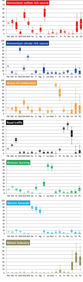
The seven-factor profiles are reported in Figs. 1 and 2. Fig-ure 1 allows factor identification, by highlighting the relative contribution of every chemical species in a given factor. Fig-ure 2 shows the contribution (in µg m−3) of chemical species to each source, i.e. the influence of each chemical compound on source contributions to PM mass. Interpreting bootstrap profiles, instead of factor profiles of the optimal base run, is preferred here as it allows uncertainties to be estimated. These uncertainties are displayed by different percentiles of bootstrap runs (Fig. 1). Figures 1 and 2 will be discussed in detail in Sect. 4.1.
Regarding factor contributions, to the best of our knowl-edge bootstrap results are not documented for the G matrix in EPA PMF3.0 output files. This thus does not allow the uncertainties associated with this G matrix to be estimated. The results given here correspond to the base run that gave the smallest Qrobust. Figure 3 and Supplement Fig. S1 re-port the daily contribution (in µg m−3) of each source to PM mass during the whole campaign; it should be recalled that some days were excluded from the data set (Supplement Ta-ble S1). Correlations between factor time series and their pre-sumable tracers are reported in Supplement Table S6. Fig-ure 4 shows the relative contribution (in %) of each source to every chemical species, giving valuable information on the apportionment of compounds emitted by different sources (e.g. OM), and on the real ability of chemical constituents to be source tracers (e.g. levoglucosan). The contribution of the unaccounted fractions (i.e. proportion of a chemical species that is not attributed to any factor) is below 5 % for most species, with the exception of nitrate, K, Cu, Pb and Cd (6, 7, 10, 13 and 17 %, respectively). Figures 3, 4 and Supplement Fig. S1 will be discussed in Sect. 4.3.
3.4 Geographical origins
The geographical distribution of the 48 h air mass back-trajectories observed during the entire project is reported in Supplement Fig. S2. On the left-hand side, a logarith-mic scale was implemented to better illustrate the number of trajectories going through each cell (nij, ranging from 0 to
3980). This figure was constructed by plotting the logarithm of (nij+1) for each cell of address (i,j). Note thatnijvalues
will be used for PSCF calculations (see Sect. 2.3.2). On the right-hand side, the number of trajectories per wind direction (nθ) is plotted and is used for CPF calculations (Sect. 2.3.1).
Regarding this last method, relatively high numbers of air mass trajectories are observed from SSW to NE sectors (ranging from 90 to 131 trajectories according to wind direc-tions), and lower numbers are reported from ENE to S sectors (from 26 to 78). Applying the weighting function defined in Eq. (4) allows CPF values to be lowered for ENE to S sec-tors. Comparable results are found with the PSCF method-ology, exhibiting a high number of trajectories per air parcel all around the region of Paris (>500) but in the S to ENE directions. Contrary to the previous figure, this illustration shows further information on the distances travelled by air masses with respect to Paris. The number of trajectories per cell is generally (i) higher than 500 from west of France to Benelux, (ii) between 50 and 500 from southwest of France, through England to Denmark and eastern Germany and (iii) lower than 20 for further geographical regions. The PSCF weighting function (Eq. 6) will again allow PSCF values to be reduced in the cells exhibiting lownij values. Hence, the
assessment of the influence of emissions from southern or eastern Europe on the city of Paris will not be possible in our study, due to the low number of trajectories per cell found in these areas, leading to a lack of statistical robustness of CPF and PSCF results.
4 Discussion
4.1 Source identification
Each PMF factor was interpreted by studying its chemical profile (F matrix). The interpretation of the seven factors will be discussed from the easiest to the most complicated PMF factor to interpret. A comparison with other European source apportionment studies will be given at the end of Sect. 4.1. 4.1.1 Biomass burning
The physical and chemical characteristics of biomass burn-ing aerosols have extensively been studied (Crutzen and Goldammer, 1993; Reid et al., 2005). Submicron particles of biomass burning origin are typically made up of OC (80 %), EC (5–9 %) and trace inorganic compounds (12– 15 %) such as potassium, sulfate, chloride and nitrate (Reid et al., 2005). Carbonaceous material (EC and a proportion of OC), potassium and chloride are likely in the particle core (Posfai et al., 2003), whereas sulfate, nitrate, organic acids and semi-volatile organic species are condensed on pre-existing particles (Reid et al., 2005). It should be noted that fuel types and combustion efficiencies will lead to a wide variety of specific chemical compositions (Fine et al., 2001, 2002, 2004). Good tracers of this source are monosaccha-ride derivatives from the pyrolysis of cellulose and hemi-cellulose, such as levoglucosan, mannosan and galactosan
(Locker, 1988; Puxbaum et al., 2007; Simoneit, 2002; Si-moneit et al., 1999).
In this study, a biomass burning (BB) source is identified through the strong presence of levoglucosan and mannosan in a single factor (84 and 80 % of their mass, respectively, Fig. 1; unless otherwise stated median values will be reported when referring to Fig. 1). In addition, noticeable proportions of potassium, OM, chloride, EC, nitrate and ammonium are present (26, 19, 15, 12, 9 and 4 %, respectively). Trace metal elements such as Pb and Ni are also observed (11 and 7 %, re-spectively) and may result from the absorption of heavy met-als present in soil and water by biomass (Sharma and Dubey, 2005). Both compounds have been found in PM2.5resulting from wood combustion in Europe (Alves et al., 2011).
Figure 2 reports the mass contribution (in µg m−3) of every chemical compound in this BB source. The major contribu-tors are OM, nitrate, EC and levoglucosan (61, 13, 9 and 7 % of the source mass, respectively; unless otherwise stated av-erage values will be reported when referring to Fig. 2), the other compounds accounting for less than 5 % by weight of this source. Hence, the wood burning contribution to PM2.5 mass is mainly governed by carbonaceous materials, and es-pecially organic matter. Interestingly, the relatively high pro-portion (by weight) of nitrate suggests that this biomass burn-ing source has undergone atmospheric ageburn-ing, implyburn-ing that BB aerosols freshly emitted by the region of Paris may not be the main contributor to this source, which is in agreement with its geographical origin (see later in Sect. 4.2) and the literature (Crippa et al., 2013a, b).
The OC / EC, OC / levoglucosan, K+/ levoglucosan ratios are 3.4, 4.7, and 0.24, respectively (with an OC-to-OM con-version factor of 1.95, Bressi et al., 2013). Only insights into the nature of this biomass source can be given through these ratios, as they are highly variable according to the type of biomass combusted (softwood, hardwood, leaves, straws, etc.), the combustion conditions, the type of locations and the measurement techniques used (especially for EC and OC concentrations). Our OC-to-EC ratio of 3.4 is of the same or-der of magnitude as the ratios reported by Schmidl (2005, cited in Puxbaum et al., 2007) for beech and spruce (2.7 and 2.6, respectively) that are widespread trees in France and neighbouring countries (Simpson et al., 1999). Our OC-to-levoglucosan ratio of 4.7 is close to the ratios reported by Schauer et al. (2001) of 3.9 and 4.3 for pine and oak, re-spectively, and by Schmidl (2005, cited in Puxbaum et al., 2007) of 5.0 for spruce. It is however lower than the rec-ommended average US ratio of 7.35 (Fine et al., 2002), and Austria ratio of 7.1 (Schmidl, 2005, cited in Puxbaum et al., 2007). Interestingly, our corresponding OM-to-levoglucosan ratio of 9.2 is close to the values of 10.3 and 10.8 estimated for fine wood burning aerosols in the region of Paris by Sciare et al. (2011) and in the French Alpine region (Greno-ble) by Favez et al. (2010), respectively. Finally, our K+ -to-levoglucosan ratio of 0.24 is in the 0.03 to 0.90 range of the different types of biomass combustion ratios compiled
by Puxbaum et al. (2007), and appears to be close to the 0.20 value reported by Schauer et al. (2001) for pine, or 0.16 value reported by Fine et al. (2001) for softwood.
To summarize, a biomass burning source was identified with the help of specific tracers, and could possibly originate from the wood combustion of trees such as beech, spruce, pine and oak (which are widespread in France and surround-ing countries), although the contribution of agricultural and garden waste burning cannot be excluded. This source has undergone atmospheric ageing, suggesting that a significant proportion is imported from outside Paris.
4.1.2 Road traffic
Road traffic aerosols are of high complexity due to the di-versity of emission processes (exhaust versus non-exhaust), and their primary and secondary natures. Tailpipe aerosols are primarily composed of OC and EC, although significant amounts of inorganic species such as ammonium nitrate can rapidly be formed by gas-to-particle conversion (Fraser et al., 1998). Non-exhaust aerosols typically arise from break wear, tyre wear, road wear and road dust abrasion, and can be dis-tinguished from exhaust aerosols by their high contents of heavy metals (e.g. Fe, Cu, Mn, Sb). However, the finding of chemical tracers related to each abrasion process still consti-tutes an active field of research (Thorpe and Harrison, 2008). In our study, the road traffic source was identified through the presence of characteristic metals and carbonaceous ma-terials. Figure 1 shows that 87, 75, 58, 41, 25, 12 and 8 % of Mn, Fe, Cu, EC, OM, Ni and Mg2+, respectively, contribute
to this source. Mn, Fe, Cu, Ni and Mg2+certainly stem from
Figure 3. Daily contribution (µg m−3) of each source to PM mass from 11 September 2009 to 10 September 2010. Note that results were taken from the base run exhibiting the lowestQrobust.
tracers mentioned in Sect. 2.1.2 might prevent us from iden-tifying a road dust fraction in this factor.
As shown in Fig. 2, road traffic source mass is essentially composed of OM and EC (63 and 28 %, respectively) and to a much smaller extent Fe (6 %). Both OM and EC are thought to stem from exhaust and non-exhaust processes in compa-rable proportions. In fact, in different European cities the contributions of exhaust and non-exhaust processes to traffic-related emissions of PM are approximately equal (Querol et
al., 2004). In addition, the importance of non-exhaust par-ticles emitted in the region of Paris has been reported in an emission inventory study (Jaecker-Voirol and Pelt, 2000). Since carbonaceous materials represent more than 90 % of our road traffic source mass, an equal contribution of both processes to OM and EC can be assumed. The low OC-to-EC ratio of 1.2 found in this source can be explained by the large proportion of diesel vehicles in the region of Paris, the low influence of secondary organic aerosols in this factor and the analytical method used to quantify both chemical com-pounds (EUSAAR_2 protocol). As a comparison, Ruellan and Cachier (2001) reported a 2.4 OC-to-black-carbon ratio near a high-flow road in Paris, Giugliano et al. (2005) a 1.3 OC-to-EC ratio at a tunnel site in Milan (Italy) and El Had-dad et al. (2009) a 0.6 value for primary vehicular exhaust emissions in France. The secondary nature of road-traffic-related aerosols will be found in other factors (see Sect. 4.1.6 for instance).
In a few words, a factor was interpreted as a road traf-fic source mainly composed of primary carbonaceous and metallic particles that are likely freshly emitted and result from exhaust and non-exhaust processes.
4.1.3 Marine aerosols
A marine aerosol source was identified by the high propor-tion of sodium, chloride and magnesium in a single factor (79, 77 and 68 %, respectively, Fig. 1). These chemical com-pounds are related to primary sea-salt aerosols produced by the mechanical disruption of the ocean surface (O’Dowd et al., 1997). The Cl−/ Na+and Mg2+/ Na+ionic ratios of 0.96
and 0.13, respectively, are on the same order of magnitude as the standard sea water composition of 1.17 and 0.11, respec-tively (Sverdrup et al., 1942; Tang et al., 1997). The lower proportion of chloride with respect to sodium can be due to acid–base reactions between sea-salt particles and sulfuric and/or nitric acids, which would lead to the evaporation of gaseous HCl into the atmosphere (Eriksson, 1959 in McInnes et al., 1994). The high sulfate-to-sodium ratio of 0.096 com-pared to 0.060 in sea water is in agreement with this assump-tion; the very high nitrate-to-sodium ratio of 1.08 likely im-plies another source for this latter compound. In fact, the amount of nitrate plus twice the sulfate formed should not exceed the chloride lost, on a molar basis.
Figure 4. Source contribution (%) of each chemical species (median of the bootstrap results,n=100). Lev: levoglucosan, Man: mannosan, Unaccounted: proportion of a chemical species that is not attributed to any factor.
and heavy metals in marine areas (Lack et al., 2009; Mur-phy et al., 2009), onto which nitrate could condense. How-ever, the presence of sulfate for both interpretations would be expected. Sea-salt particles could also be enriched by an-thropogenic compounds during their transport from marine regions to Paris, due to inland emissions (e.g. of EC, Ni, K, Cu) from combustion processes. Finally, uncertainties related to PMF simulations should not be excluded as well (e.g. the slope of the linear regression between observed and predicted concentrations for chloride and EC are 0.62 and 0.68, respec-tively, Table 1).
The resulting mass contributions to this source are 0.2±0.1, 0.2±0.1 and 0.1±0.0 µg m−3for OM, nitrate and EC, respectively, 0.2±0.0 and 0.2±0.02 µg m−3 for Na+
and Cl−, respectively, and minor for the other compounds
(Fig. 2). The primary sea-salt fraction of this source (Na+,
Cl−and Mg2+) hence accounts for ca. 37 % of its mass and the likely anthropogenic fraction (EC, OM and nitrate) for the other 63 %.
In conclusion, a marine aerosol source comprising sea-salt particles and a large fraction of anthropogenic aerosols – which could possibly originate from combustion processes – has been identified.
4.1.4 Heavy oil combustion
A strong proportion of V, Ni and SO24− (87, 64 and 33 %, respectively) is found in a single factor. Vanadium and nickel are primarily emitted by heavy oil combustion, whose sources are industrial boilers (e.g. used in refineries), elec-tricity generation boilers (e.g. oil power stations), large ship-ping ports, etc. (Jang et al., 2007; Moreno et al., 2010; Pa-cyna et al., 2007). It is difficult to distinguish between these sources, and “heavy oil combustion” seems to be the most suitable label for this factor. The presence of a significant
proportion of sulfate is in agreement with most source ap-portionment studies that have identified this type of source (e.g. Vallius et al., 2005; Viana et al., 2008). A part of ammo-nium, OM, EC, Mg2+and Fe is also noticeable (17, 16, 15, 13 and 9 %, respectively). Typical fuel oils naturally contain carbonaceous material, but also magnesium and iron (Miller et al., 1998), whereas ammonium is a secondary compound resulting here from the reaction with acidic sulfate to form ammonium sulfate. Larger uncertainties are associated with the other chemical elements (e.g. 25th–75th percentiles of 1– 32, 2–25 and 0–12 % for Cd, Pb and Cu, respectively), which will therefore not be regarded as part of this factor.
4.1.5 Metal industry
As shown in Fig. 1, strong proportions of Cd, Pb and Cu are found in the same factor (47, 32 and 16 % of their mass, re-spectively), although high interquartile ranges are observed (25th–75th percentiles of 29–55, 21–45, and 9–30 %, re-spectively). High uncertainties are thus associated with this source, which is partly due to the difficulty of PMF to model cadmium (coefficient of determination of 0.58 for observed versus predicted concentrations, see Table 1). Cadmium and lead emission inventories have been reported for Europe by Pacyna et al. (2007) for the year 2000. The major sources of heavy metals have been taken into account, including com-bustion of coal/oil in industrial, residential and commercial boilers, iron and steel production, waste incineration, gaso-line combustion, etc. Although substantial uncertainties are associated with each emission category (e.g.±20 % for sta-tionary fossil fuel combustion,±25 % for iron and steel pro-duction), they conclude that the main source of cadmium is fuel combustion to produce heat and electricity (62 % by weight), whereas Pb is first emitted by gasoline combustion (51 %).
The Pb / Cd ratio can be further investigated to discrim-inate between these types of sources. In our study, the Pb / Cd ratio is 27 on average (weight / weight ratio), which is far lower than the expected value for gasoline combustion aerosols (2300), but closer to the mean ratio of anthropogenic European emissions (46), and to the low range of values (5– 15) reported for non-ferrous metal production (Dulac et al., 1987; Pacyna, 1983). This is in agreement with the geograph-ical origins of this source (see later in Sect. 4.2). The high-est mass contributions to this source are attributed to OM, nitrate, sulfate and EC (0.03, 0.03, 0.02 and 0.01 µg m−3, respectively, Fig. 2). Very high uncertainties are associated with these concentrations that are close to, or lower than, method quantification limits. The overall contribution to PM mass is negligible (0.10 µg m−3).
To summarize, this PMF “metal industry” source presum-ably reflects a mesoscale background aerosol, composed of a high proportion of heavy metals that likely originate from industrial activities (non-ferrous metal production, industrial boilers, etc.).
4.1.6 Ammonium nitrate (A.N.)-rich factor
The majority of nitrate and ammonium is found in a sin-gle factor (75 and 52 %, respectively) while an important proportion of sulfate is also present (17 %). Smaller con-tributions of Cd, Mn, Cl−, K+ and OM are also observ-able (9, 9, 7, 6 and 5 %, respectively). Figure 2 shows that nitrate, ammonium, sulfate and OM account for 2.0±0.2, 0.7±0.1, 0.4±0.1 and 0.3±0.2 µg m−3, respectively. This source thus represents secondary inorganic aerosols, with a stronger proportion of ammonium nitrate than ammonium sulfate, the latter being discussed in detail in the following
section (Sect. 4.1.7). Ammonium nitrate stems from chem-ical reactions between ammonia and nitric acid, the latter compound resulting from the oxidation of NOx (NO and NO2) (Schaap et al., 2004). It therefore appears necessary to identify the major sources of NOxand ammonia to know the sources of this factor.
In Europe, atmospheric ammonia is predominantly emit-ted by agricultural activities – such as volatilization from an-imal waste and synthetic fertilizers – which have been esti-mated to contribute 94 % of their mass emissions in 2004 for example (Pay et al., 2012). In France, emission inventories also reach the same conclusion, with agricultural activities accounting for 97 % of total emissions during the same year, but also during the years 2009 and 2010 corresponding to this study (CITEPA, 2012). Other sources of ammonia such as biomass burning, fossil fuel combustion, natural emissions, etc. (Krupa, 2003; Simpson et al., 1999) will thus not be re-garded as contributing to ammonia emissions here.
On the other hand, NOx is produced by a variety of sources, including the combustion of fossil fuel, biomass burning, lightning, microbiological emissions from soils, etc. (Lee et al., 1997; Logan, 1983). In Europe, based on emis-sions of 2004 reported by Pay et al. (2012), the major anthro-pogenic sources of NOxare road and non-road transport (33 and 31 %, respectively), followed by energy transformation and industrial combustion (17 and 11 %, respectively), using the Selected Nomenclature for Air Pollution. In France, us-ing a slightly different nomenclature (so-called SECTEN), CITEPA (2012) reported that, for the selected years 2004, 2009 and 2010, NOxemissions primarily stemmed from road transport (55 %), manufacturing industry (13–15 % depen-dant on the year), agriculture (9–10 %), residential and ser-vice sectors (7–10 %) and energy transformation (8–9 %). The heavy metals present in this factor presumably come from some of the aforementioned activities such as road transport, manufacturing industry, and energy transforma-tion. In addition, although they are not referred to in these emission inventories, the possible contribution of biomass burning in this factor should not be excluded, as suggested by the presence of potassium, chloride and OM. In that case, the unexpected absence of levoglucosan and mannosan could be explained by the imported nature of this source (see Sect. 4.2), which could lead to the degradation of these tracers during their transport (Hoffmann et al., 2009, see Sect. 4.1.7 for further details).
4.1.7 Ammonium sulfate (A.S.)-rich factor
This last factor is certainly the most complicated to interpret given the high proportions of miscellaneous chemical com-pounds (Fig. 1), implying the contribution of a wide variety of sources. A strong proportion of K+, SO24−, OM, NH+4, Pb, EC and Cd (54, 46, 29, 26, 24, 17 and 17 %, respectively) and a smaller fraction of Mg2+, Na+, Ni and Fe (17, 8, 6,
5 and 5 %, respectively) are observed. Mass contributions to this source are dominated by OM, SO24−, NH+4 and EC (1.6±0.3, 1.0±0.2, 0.4±0.1 and 0.3±0.2 µg m−3, respec-tively, Fig. 2). Based on these data, we will try to associate chemical compounds likely to result from the same source.
Sulfate is certainly primarily bound with ammonium – (NH4)2SO4– as aerosols sampled in Paris are neutral, and as ammonium neutralizes most of nitrate and sulfate (Bressi et al., 2013). Ammonium sulfate aerosols come from the chemical reaction between ammonia and sulfuric acid, the latter compound resulting from the oxidation of sulfur diox-ide. Ammonia is almost exclusively emitted by agricultural activities as mentioned in the previous section, whereas sul-fur dioxide is principally emitted by energy transformation (56 %), non-road transport (17 %) and industrial combus-tion (13 %), according to the aforemencombus-tioned study of Pay et al. (2012). In France, CITEPA (2012) states that energy transformation (54 %) and the manufacturing industry (30 %) are the main sources of SO2(in 2009), without taking into account maritime transport. These industrial activities could explain the presence of metals such as Ni, Cd, Fe and Pb, as well as a fraction of carbonaceous matter in this factor. Ni, Cd, Fe and Pb might also come from coal burning emissions (Junninen et al., 2009) which could have been transported from central/eastern Europe to Paris (see Sect. 4.2.).
The substantial presence of potassium is presumably re-lated to biomass burning emissions. The absence of levoglu-cosan and mannosan is unexpected but could be explained by their degradation during transport due to oxidative re-actions with OH radicals (Hoffmann et al., 2009; Kundu et al., 2010), as this source is thought to be mainly imported (Sect. 4.2). For instance, the seasonal average levoglucosan concentration of our data set (13.5 and 411.8 ng m−3in sum-mer and winter, respectively) could be degraded in less than 2 h in summer, and less than 2.5 days in winter (57 h), fol-lowing the degradation rates given in Hoffmann et al. (2009) of 7.2 ng m−3h−1and 4.7 ng m−3h−1in summer and winter, respectively. The aged property of biomass burning particles contributing to this source is in line with the absence of chlo-ride in this factor, which could be due to the chemical conver-sion of KCl particles to K2SO4(or to a lesser extent KNO3), after having undergone similar heterogeneous reactions men-tioned for marine aerosol particles in Sect. 4.1.3 (Li, 2003). The aforementioned study reported that more than 90 % of KCl particles coming from biomass burning were converted to potassium sulfate or nitrate after only 24 min in south-ern Africa. Nevertheless, given the geographical origins of
this source, we do not exclude the potential contribution of potassium industries (e.g. fertilizer industries) in this source as well, which could produce potassium sulfate and potas-sium nitrate compounds.
Finally, because of the high proportions of sulfate and ammonium, this source is essentially secondary in nature. Therefore, OM can here be assumed to principally refer to secondary organic aerosols (SOAs), as it is supported by the high OM-to-EC ratio of 5.6. The complexity and the multi-plicity of the chemical processes leading to the formation of SOA do not allow us to determine its precise sources. Beek-mann et al. (2014) reported that SOA could be of mixed an-thropogenic (fossil fuel) and biogenic origins in the region of Paris (see also Crippa et al., 2013a, b on this subject).
To summarize, this factor is primarily made of secondary aerosols, which stem from a variety of sources includ-ing agriculture, industrial activities, non-road transport and biomass burning, to name a few.
4.1.8 Comparison with other source apportionment (SA) studies
4.2 Source geographical origins
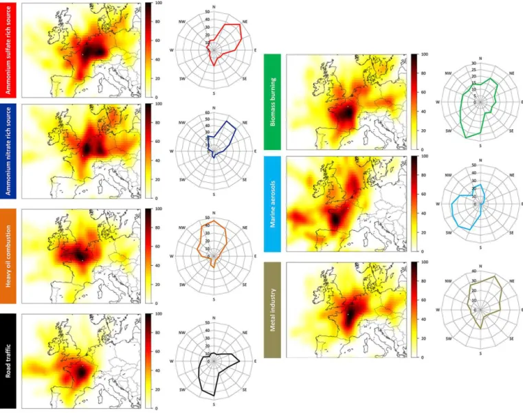
The geographical origins of each PM2.5source determined by PSCF and CPF are reported in Fig. 5. This figure aims at providing insights on source localization but does not claim to be accurate at the pixel or the degree level. PSCF and CPF results will first be compared, and only similar results will be further interpreted for each source. Note that the values of the probabilities given by PSCF and CPF are not directly com-parable as weighting functions, and smoothing procedures differ from one methodology to the other.
Regarding the A.S.-rich factor, the high probability it comes from geographical regions located northeast of Paris is highlighted by both methodologies. In fact, the probabil-ities for this factor to exceed the 75th percentile in CPF are clearly higher for air masses coming from NNE to ENE than from other directions (40 versus 12 % on average, respec-tively). Similarly, a hot spot is observable in this NE direction with PSCF, with probabilities to exceed the aforementioned criterion being higher than 80 % from northeast of France to Benelux and southwest Germany. Interestingly, these ge-ographical regions are amongst the major emitters of sulfur dioxide in Europe (Pay et al., 2012), which is – with ammo-nia – a precursor of ammonium sulfate. High probabilities (ca. 55 %) are however observed with PSCF for almost all of France and southeast England, contrary to CPF. Given the long lifetime compounds present in this factor, it is possi-ble that its high contributions result from anticyclonic condi-tions, involving stagnating air masses that could come from any regions around Paris. In addition, because such results are not observed in CPF, bias related to the binomial smooth-ing used in PSCF may not be excluded.
The A.N.-rich factor is likely coming from regions lo-cated NNE of Paris. Conditional probability function values are significantly higher for NNE and NE than for the other directions (49 versus 11 % on average, respectively). Sim-ilarly, PSCF probabilities are the highest in this direction (generally above 60 %), against probabilities generally be-low 20 % in the other directions. This is also in line with the European map depicted by Pay et al (2012) for total nitrate (HNO3+ NO−3) concentrations, which appear higher in this geographical area.
The heavy oil combustion source presumably comes from north of France although a local influence is not excluded. Conditional probability function suggests this source origi-nates from NNW to NNE directions (mean of 42 % against 12 % for the other directions), and PSCF shows its high-est probabilities in the NNW direction (higher than 80 % in northern France and the English Channel). Northern France comprises some of the largest harbours of the country (e.g. Le Havre, Dunkirk, Calais) and is a highly industrial-ized region (e.g. the Nord-Pas-de-Calais region, located near Belgium and the English Channel is the fourth largest indus-trialized French region). These activities are in line with the industrial feature of this source mentioned in Sect. 4.1.4, and
will be further discussed in Sect. 4.3.1. On the other hand, the high PSCF values observed in the English Channel sug-gest that maritime transport clearly affects the contribution of this factor. The low V-to-Ni ratio reported in our study (Sect. 4.1.4) thus might not be the best proxy to distinguish between industrial and maritime heavy oil combustion. Fi-nally, influences of local sources cannot be excluded as well, given the high number of industrial activities in the region of Paris. As PSCF and CPF only focus on the highest contri-butions of sources, local emissions could be omitted by both methodologies, because they would constantly increase the concentrations of this factor without however triggering pol-lution events.
The road traffic source is primarily of local origin. Never-theless, CPF and PCSF also indicate the influence of central France, which is unlikely and could be related to an arte-fact discussed below. High probabilities are observed with CPF for S to SSW (42 % on average) and E directions (33 %) compared with the other air mass origins (16 % on average). Potential source contribution function probabilities are also higher for S to SW directions (above 80 %), but contrary to CPF the eastern direction is not highlighted here. Instead, moderate probabilities are rather uniformly distributed all around the region of Paris (ranging from 50 to 70 %) that could be related to a local origin for this source. The eastern influence shown by CPF will not be regarded as meaning-ful given its divergence with PSCF values. Differences be-tween both methodologies could also be related to the local feature of this source. In addition, it is very unlikely that pri-mary particles with road transport characteristics measured in Paris were imported from central France given the high number of vehicles present in the megacity. Furthermore, a comparison between our EC concentrations (45 % of EC is found in this factor; Fig. 4) and those measured at a rural site located 60 km southward does not show any correlation (r2=0.03, slope = 0.27, n=335, Bressi et al., 2013). In-stead, air masses originating from south of Paris could be related to low boundary layer heights (BLHs) that would en-hance local road traffic aerosol concentrations. We attempted to quantify this phenomenon and found that 40 % of back-trajectories coming from south of Paris (n=123) display BLH below 600 m (corresponding to 26th percentile of BLH values measured during the campaign; see Bressi et al., 2013, for further information on BLH measurements). Other mete-orological parameters (e.g. atmospheric pressure) should be taken into account to fully understand the characteristics of these air masses stemming from south of Paris.
Figure 5. Probability (in %) that the contribution of a source exceeds the 75th percentile of all its contributions, when air masses came from a given air parcel (left, PSCF), or a given wind direction (right, CPF). Note that the city of Paris is indicated by a grey dot on PSCF figures; for each source, PSCF probabilities have been normalized to 100 %.
homogeneous probabilities all around Paris (ca. 60 %) with however significantly higher values south to southwest of this megacity (higher than 80 %). Two assumptions could explain such results. First, this BB source could be locally emitted as suggested by relatively isentropic results for both approaches with the exception of S to SW directions. In that case, the hot spot highlighted S to SW of Paris would be due to the same feature described previously for the road traffic source (specific meteorological conditions such as low BLH related to air masses stemming from south of Paris). This assumption is in line with previous studies stating that BB aerosols are locally emitted in the region of Paris (Favez et al., 2009; Sciare et al., 2011). Second, a proportion of this source could actually be imported from south of Paris. This is supported by a comparison conducted between atmospheric concentrations of levoglucosan measured at our urban site
and at the aforementioned rural site (located 60 km south of our sampling site). Very good correlations are observed between both data sets on the entire duration of the project (r2=0.84, slope = 0.84, n=331; Beekmann et al., 2014), suggesting that a noticeable proportion of biomass burning aerosols could be imported from south of Paris. Further re-search should be conducted on biomass burning sources in Paris to fully explain this surprising influence of geographi-cal areas located south of Paris.
probabilities from the Atlantic Ocean to western France (above 80 %), intermediates in the North Sea (ca. 60 %) and low values from NE to S (typically below 20 %). Interest-ingly, the hot spot highlighted in the Atlantic Ocean corre-sponds to a geographical area where the biggest salt ponds in the country lie (e.g. Guérande, Noirmoutier). As suggested by high PSCF probabilities in western France, the anthro-pogenic fraction of this source most plausibly stems from inland anthropogenic emissions that could be (internally or externally) mixed with sea-salt particles, or could affect their chemical composition.
Lastly, the metal industry source seems to reflect a re-gional haze, although the influence of areas located northeast of Paris is underlined. Conditional probability function dis-plays higher probabilities from NNW to NE than for the other directions (31 versus 14 % on average, respectively). Poten-tial source contribution function also points to high prob-abilities in the NE direction with values higher than 80 % in northeastern France. Contrary to CPF, Paris and central France also exhibit high PSCF values (above 80 %). Discrep-ancies observed between CPF and PSCF results might reflect the presumably regional background properties of this factor, characterizing a mesoscale haze of metal industry emissions. They could also be due to the very low atmospheric concen-trations of this source (representing 1 % of PM2.5 mass on average) leading to large uncertainties.
4.3 Source contribution 4.3.1 Annual average
The annual average contribution of the seven sources to PM2.5mass is reported in Fig. 6. The two predominant fac-tors are the ammonium sulfate and the ammonium nitrate-rich factors accounting for ca. half of PM2.5 mass (51 %). Heavy oil combustion, road traffic and biomass burning also contribute significantly to fine aerosol mass (17, 14 and 12 %, respectively), whereas marine aerosols and metal industry sources have a far lower contribution (6 and 1 %, respec-tively). These contributions were compared with source ap-portionment studies (see Fig. 7 and Supplement Table S7), chosen according to the following criteria:
(i) SA is performed on PM mass (PM2.5 in most of the cases);
(ii) each SA study is representative of a 1-year minimum; (iii) when possible, SA studies have been chosen according
to their presumable geographical origins (e.g. continen-tal Europe for A.S.- and A.N.-rich sources);
(iv) similar source categories (i.e. factor identifications) are reported.
The prevalence of an ammonium sulfate-rich factor in European SA studies is widely reported (Viana et al.,
Figure 6. Annual average contribution (µg m−3; %) to PM2.5mass (14.7 µg m−3) of the seven sources, from 11 September 2009 to 10 September 2010.
2008). It is, for instance, illustrated in a study conducted by Mooibroek et al. (2011) on PM2.5 sampled over 1 year (2007–2008), at five sites in the Netherlands (one urban, one kerbside and three rural sites). An A.S.-rich factor was identified by EPA PMF3.0, and contributes from 20 to 30 % of PM2.5mass, with a PM2.5 annual average concentration ranging from 12.5 to 17.5 µg m−3(i.e. on the same order of magnitude as our mean PM2.5level of 14.7 µ g m−3). The ab-solute contributions of this source are 4.4 and 4.9 µg m−3at two rural sites (Vredepeel and Cabauw sites, respectively; values calculated from concentrations given in Weijers et al., 2011), which is higher than the contribution of 3.9 µg m−3 re-ported in our study. Interesting results are also rere-ported in an SA study conducted at an urban background site in Copen-hagen (Denmark) by Andersen et al. (2007). The comparison with our results is much more limited here, as this study was conducted on PM10, for a 6-year period (1999–2004), and as a hybrid receptor model combining chemical mass balance (CMB) and PMF approaches (COPREM model) was used. Nevertheless, most of the compounds found in our A.S.-rich factor (ammonium sulfate and SOA) are assumed to be in the fine mode, and the sources identified with COPREM are very similar to ours. The resulting contribution of their A.S.-rich factor is 3.5 µg m−3, which is again close to the value of 3.9 µg m−3reported in our study. The contribution of the am-monium sulfate-rich factor to PM2.5mass found in our work is hence in the range of values reported in other European SA studies, and the presumable influence of countries located northeast of France appears relevant, regarding the high con-tributions of this A.S. factor in this geographical area.
The A.N.-rich factor is also a predominant contributor to PM2.5 in European SA studies (Viana et al., 2008). Mooibroek et al. (2011) report a very high contribution of this source in the Netherlands, ranging from 5.6 to 7.7 µg m−3according to sites, compared to a contribution of 3.5 µg m−3in our study. Andersen et al. (2007) report a con-tribution of 3.3 µg m−3on average in Copenhagen, which is in line with our value.
Figure 7. Comparison of the contribution (in µg m−3) of the major sources of PM determined by receptor model studies at different European locations (see Bressi, 2012, Supplement Table S6 and text for more details). Note that sites are indicated as follows: “City (Country)-Type of site”. Urb: urban, Rur: rural, Kerb: kerbside.
common sources of precursor gases and are imported from the same geographical area in our study (see Sects. 4.1.6, 4.1.7 and 4.2). A secondary aerosol source was identified by Quass et al. (2004) with PMF in Duisburg (Germany), based on 1-year measurements of PM2.5(2003–2004). Its annual contribution to PM2.5mass is higher than the value reported in our study (57 % versus 51 %, respectively), as are its abso-lute concentrations (13.0 µg m−3versus 7.4 µg m−3, respec-tively). On the other hand, Vallius et al. (2005) reported at an urban site in Amsterdam (study conducted from Novem-ber 1998 to June 1999) a contribution of a PM2.5secondary aerosol source of 6.8 µg m−3that is comparable to ours. Fi-nally, the summed contribution of A.S. and A.N. factors reaches 6.8 µg m−3 in the study of Andersen et al. (2007), and ranges from 8.6 to 12.6 µg m−3 according to sites in Mooibroek et al. (2011). Therefore, the predominant con-tribution of secondary aerosol sources to fine aerosol mass estimated in Paris is in line with most SA studies conducted in Europe. The high proportions of such sources in countries located northeast of France support the idea that this region significantly affects secondary aerosol concentration levels measured in Paris.
Regarding the heavy oil combustion source, its impor-tant contribution to PM2.5 mass of 17 % (2.4 µg m−3) is relevant with its imported feature from northern France (cf. Sect. 4.2), where there is a high density of industries and strong emissions from maritime transport in the English Channel. The influence of industrial activities on aerosol lev-els in this geographical area has been reported by Alleman et al. (2010) in a study conducted in the highly industrial-ized harbour of Dunkirk, which is one of the largest French commercial harbours (freight transport: 58 million tonnes
combustion sources to fine aerosols should be conducted in the region of Paris, given the surprisingly high levels found in our study.
The road traffic source contributes 14 % of PM2.5 mass which represents 2.1 µg m−3. This contribution is noticeable, but was expected to be more important given the high den-sity of vehicles in Paris. It is, for instance, markedly lower than the 3.8 µg m−3estimated by PMF for PM1.0though, at an urban background site in Zurich (Switzerland) by Min-guillón et al. (2012) from a winter and summer campaign. It is also significantly lower than the 7.8 µg m−3 estimated by CMB for PM2.5, at an urban background site in Milan (Italy) by Perrone et al. (2012) for a 3-year period (2006– 2009). As mentioned in Sect. 4.1.2, the absence of a road dust fraction might partly explain the relatively low contri-bution of our road traffic source. Nevertheless the level es-timated in our study is comparable with other highly popu-lated urban areas in the world. For instance, at an urban site in Toronto (Canada, ca. 5.6 million inhabitants in the metropoli-tan area), from PM2.5sampled over 1 year (2000–2001), Lee et al. (2003) apportioned an estimated 2.3 µg m−3 contribu-tion to a road transport source using PMF. Their resulting contribution to PM2.5 mass is slightly higher than ours (18 versus 14 %, respectively). Similar levels were also reported in Seattle (US, ca. 3.5 million inhabitants in the metropolitan area) by Maykut et al. (2003) from multi-annual measure-ments (1996–1999) conducted at an urban site. The PMF and UNMIX approaches lead to a contribution of 2.0 and 2.5 µg m−3for this source, i.e. 22 and 28 % of PM2.5mass respectively.
The biomass burning source is the last considerable con-tributor to PM2.5in Paris (12 %, 1.8 µg m−3). To the best of our knowledge, the contribution of such source to particu-late matter mass in Paris is estimated for the first time on the annual scale in our study. However, two studies attempted to estimate it from campaigns of few days or weeks (Favez et al., 2009; Sciare et al., 2011) that do not allow suitable comparisons to be performed on the annual scale. (Note that comparisons will nonetheless be conducted in the next sec-tion on the seasonal scale only.) In Europe as well, few stud-ies report the contribution of BB to PM mass. Andersen et al. (2007) estimated a very large contribution of 7.3 µg m−3 for this BB source, representing 15 % of their PM10 sam-ples in Copenhagen. Note that biomass burning sources are presumably entirely found in the fine fraction (e.g. Karana-siou et al., 2009), making the previous comparison relevant. Perrone et al. (2012) also report a substantial contribution of 7.1 µg m−3 representing 16 % of their PM
2.5 samples in Milan (Italy). Finally, Karanasiou et al. (2009) estimated by PMF this contribution to be 0.8 µg m−3in Athens (Greece), representing 15 % of their PM2.0samples.
The contribution of the marine aerosol source is fairly low (6 %, 0.8 µg m−3), likely because its mass size distribution is mainly located in the coarse mode. It is comparable to values reported in the Netherlands (e.g. 0.8 µg m−3 at a rural site,
Figure 8. Variations of the seasonal averaged contributions (µg m−3) of the seven sources of PM2.5. Note that calendar seasons were used (see Table 3 for more details).
Mooibroek et al., 2011), in Finland (0.9 µg m−3at an urban site of Helsinki, Vallius et al., 2003) or in Greece (1.1 µg m−3 at an urban site in Athens, Karanasiou et al., 2009). This comparison however presents some limitations since the dis-tance from the coast is substantially higher for our sampling site (ca. 300–500 km depending on the direction) compared to the aforementioned sites (around or below 100 km). Fi-nally, metal industry contributes very low levels of PM2.5 in our study (1 %, 0.1 µg m−3) that certainly reflects a haze due to large-scale pollution, as it is reported in Poulakis et al. (2014).
4.3.2 Seasonal variability