www.atmos-meas-tech.net/7/3445/2014/ doi:10.5194/amt-7-3445-2014
© Author(s) 2014. CC Attribution 3.0 License.
Improving the bias characteristics of the ROPP refractivity
and bending angle operators
C. P. Burrows1, S. B. Healy2, and I. D. Culverwell1 1Met Office, Exeter, UK
2ECMWF, Reading, UK
Correspondence to:C. P. Burrows ([email protected])
Received: 21 March 2014 – Published in Atmos. Meas. Tech. Discuss.: 6 May 2014 Revised: 1 August 2014 – Accepted: 18 August 2014 – Published: 9 October 2014
Abstract.The bending angle observation operator (forward model) currently used to assimilate radio occultation (RO) data at the Met Office, the European Centre for Medium-Range Weather Forecasts (ECMWF) and other centres is the same as is included in the Radio Occultation Process-ing Package (ROPP), along with the correspondProcess-ing tangent-linear and adjoint code. The functionality of this package will be described in another paper in this issue. The mean bending angle innovations produced with this operator using Met Office background fields show a bias that oscillates with height and whose magnitude peaks between the model levels. These oscillations have been attributed to shortcomings in the assumption of exponentially varying refractivity between model levels. This is used directly in the refractivity operator, and indirectly to produce forward-modelled bending angles via the Abel transform. When the spacing between the model levels is small, this assumption is acceptable, but at strato-spheric heights where the model level spacing is large, these biases can be significant, and can potentially degrade anal-yses. This paper provides physically based improvements to the functional form of refractivity with height. These new assumptions considerably improve the oscillatory bias, and a number of approaches for practical implementation of the bending angle operator are provided.
1 Introduction
A key feature of radio occultation (RO) data is that the raw observations of excess phase should be unbiased, due to the use of an atomic clock onboard the low Earth orbiting (LEO) RO receiver. These raw measurements, however, are
not straightforward to assimilate into a numerical weather prediction (NWP) system, and the raw data are usually pre-processed into bending angles or refractivities, which are then disseminated on the Global Telecommunication System (GTS).
Data assimilation (DA) is the process of producing a sta-tistically optimal “analysis” which is used as an input to an NWP forecast system. The assimilation step blends infor-mation from observations and short range (e.g. 6 h) forecast fields, i.e. the background. Mathematically, the basic, time-independent DA problem is defined as finding the value ofx
which minimises the following cost function,J:
J (x)=1
2 h
(xb−x)TB−1(xb−x)+ (1)
(y−H (x))TR−1(y−H (x))i,
wherexis the model state vector,xbis the background state vector (i.e. the “first guess”),yis the observation vector,H
cost function depends on the “innovations”, i.e. y−H (x)
and not simply the observations themselves. For this reason, it is just as important to ensure that the forward modelH is accurate as it is to ensure that the observations are of good quality. This paper will discuss improvements to the RO re-fractivity and bending angle forward models which are used at several NWP centres and form part of the Radio Occul-tation Processing Package (ROPP), henceforth referred to as the “ROPP operator” for brevity.
In the case of refractivity assimilation, the observed re-fractivity values describe the atmosphere at particular points (with some degree of spatial correlation), so interpolation of refractivity to this point is necessary. Forward-modelled bending angles, however, depend on the entire model atmo-sphere above the tangent point (Fjeldbo et al., 1971). For this reason, the variation of refractivity with height needs to be known at all heights, from the tangent point to the top of the model, including all points between the model levels. This is necessary in order for the Abel integral, which cal-culates bending angles from refractivity, to be evaluated (see Sect. 3).
The ROPP operator is based on Healy and Thepaut (2006). This assumes exponentially varying refractivity,N, as a func-tion ofxbetween model levelsiandi+1. The independent variablexis the product of the refractive indexnand the dis-tance from the local centre of curvature of the Earth r, i.e.
nr:
N (x) = Niexp(−ki(x−xi)) for xi≤x < xi+1, (2) where
ki =
ln(Ni/Ni+1)
xi+1−xi
. (3)
This ensures continuity at the model levels: N (xi)=Ni
andN (xi+1)=Niexp(−ki(xi+1−xi))=Ni+1.
With some further approximations, this variation of N
with height can allow the bending angle to be calculated via the Abel transform, resulting in a difference of error func-tions, see Eq. (9) (Healy and Thepaut, 2006). To a first ap-proximation the exponential assumption seems reasonable as the refractivity is given by
N =c1
P T +c2
Pw
T2, (4)
whereP is pressure,T is temperature,Pwis the partial pres-sure of water vapour and c1 andc2 are empirical constants (Smith and Weintraub, 1953).
In a dry atmosphere, the first term in Eq. (4) effectively represents the mass field. Where the temperature is constant, the hydrostatic equation dP /dz= −ρgimplies that P falls exponentially with height:P (z)=Piexp(−gz/RT ).
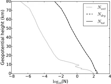
There-fore,N also falls exponentially. This behaviour can be seen in Fig. 1 for a typical example of how model refractivity varies with height. If the spacing between model levels is
Figure 1.Logarithm (base 10) of a randomly selected (but fairly typical) vertical refractivity profile, forward modelled from a 70-level Met Office background profile. This highlights the approxi-mately exponential behaviour of refractivity with height. The dry and wet terms have also been plotted to show their relative contri-butions.
sufficiently small, this assumption can produce reasonable refractivities between the levels, and hence bending angles. If the spacing is large, however, the innovation statistics show features which indicate failings of this assumption. This pa-per aims to address refinements to the form of the refrac-tivity with height used in the refracrefrac-tivity and bending angle forward models.
2 Refractivity
Currently, bending angles are assimilated operationally at the Met Office but from 2006 to 2010 refractivity data were as-similated, and some NWP centres continue to assimilate re-fractivity operationally. To forward model rere-fractivity at an observation height which lies between two model levels, the same exponential assumption was applied (i.e. Eq. 2, but in terms of geopotential height). This is equivalent to perform-ing a linear interpolation of ln(N )between the two model levels surrounding the observation height.
Nob_height=expŴln(Ni)+(1−Ŵ)ln(Ni+1), (5) where
Ŵ=Zi+1−Zob_height Zi+1−Zi
. (6)
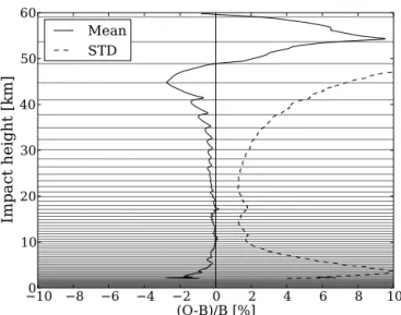
Figure 2.Refractivity innovations from 25 Met Office (6-hourly) model cycles, with observation data from all available RO instru-ments. The period started with the 00 Z analysis on 1 January 2014. The refractivity between model levels is calculated using Eq. (2). Typical heights of the model levels are overlaid as horizontal lines.
this context,Bdenotes the simulated observations forward-modelled from backgrounds, H (x), on observation levels and not the background error covariance as above.
The values of(O−B)/Bare calculated for each observed profile (i.e. in observation space), where the background pro-files are horizontally interpolated from full-resolution (70-level) Met Office fields. The(O−B)/Bvalues are then verti-cally interpolated linearly onto a fixed grid with 100 m spac-ing for statistics to be calculated (mean and standard devi-ation), thus allowing profiles with different sets of impact heights to be included in the statistics. All plotted(O−B)/B
statistics in this paper are calculated this way.
The bias above∼45 km should be ignored as it is due to a Met Office-specific model temperature bias, which is an-ticipated to improve with an upcoming model upgrade. Sim-ilarly, the growing negative bias above ∼17 km relates, at least partly, to a bias arising from the handling of Met Office levels in the refractivity forward model. This broad bias is potentially problematic, but is specific to the Met Office. The cause is understood and is being addressed but is largely in-dependent of the main topic of this paper, so will be ignored to avoid complicating the discussion.
The general issue that will be addressed here is the small-scale undulation that is present in the bias and is most notice-able between 25 and 45 km. The origin of these fluctuations is clear when the model levels are overlaid, as in Fig. 2.
It can be seen that the magnitude of the oscillatory signal is smallest when the observations are close to the model levels and largest in between. This is a real bias and not a feature of the plotting (the plotting routines have no knowledge of the heights of the model levels, and work entirely in observation
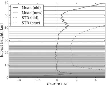
Figure 3.Bending angle innovations from the same period as Fig. 2, with typical model levels overlaid. The functional form of refractiv-ity used in the Abel integral is Eq. (2). Note that the model levels are plotted on geopotential heights and not converted to impact heights.
space). In a DA system (3D-Var for simplicity), the cost func-tion takes the form of Eq. (1). Therefore, the oscillafunc-tions in the innovations (y−H (x)) will be present in this quantity, and hence they will introduce biases into the DA system.
The origin of these oscillations is apparently the exponen-tial assumption between model levels.
3 Bending angle
The bending angle forward model is much more sensitive to subtle changes in the model background and the form of dN (x)/dx which is integrated above the tangent height, i.e. the bending angle depends on the vertical gradient of the re-fractivity. Therefore, it is no surprise that the bending an-gle statistics show the oscillatory bias even more strongly in Fig. 3.
These statistics are calculated in a similar way to refractiv-ity (above), but the values of(O−B)/Bfor each profile are interpolated to a fixed grid of impact heights (impact parame-ter minus the local radius of curvature) rather than geopoten-tial heights. These fixed heights are spaced by 100 m. Plot-ting bias statistics with coarse vertical binning (e.g. 1 km) can hide these features, so we encourage other NWP centres to follow this methodology to avoid overlooking similar os-cillations.
The bending angle as a function of impact parameterα(a)
is given by the Abel integral (Fjeldbo et al., 1971; Melbourne et al., 1994; Kursinski et al., 1997):
α(a)= −2a
∞ Z
a
d lnn
dx
√
wherex=nras before. By assuming exponential refrac-tivity, and assuming √x2−a2≃√2a√x−a, the bending angle contribution from a single layer is given by Healy and Thepaut (2006):
1αi=10−6
p
2π akiNiexp{ki(xi−a)} × (8)
h
erfnpki(xi+1−a) o
−erfnpki(xi−a)
oi
. (9)
The implementation of the error function uses an accurate fit (Eq. 7.1.25, Abramowitz and Stegun, 1965) to minimise the computational cost.
Because this is an integral from the tangent height upwards and is weighted most strongly close to the tangent point by the denominator, it is expected that if the assumption of ex-ponential refractivity between model levels is less than ideal, then the magnitude of the bias would be smallest close to the model levels, where N (x) is the best representation of the model field (i.e. without any additional distortion from the vertical interpolation), and largest in between. This can be seen in Fig. 3, though unlike the refractivity statistics, the os-cillations in the bending angle bias are not symmetric about the centres of the layers. Interestingly, these oscillations do not appear so prominently in the equivalent statistics from the European Centre for Medium-Range Weather Forecasts (ECMWF) – results suggest that this is due to the higher ver-tical resolution (more than two times larger) in the strato-sphere compared to the Met Office, making the exponential assumption more accurate. This is discussed later in this pa-per.
The bending angle operator proposed by Cucurull et al. (2013) assumes a cubic representation of refractivity as a function of height. This implementation ensures that the ver-tical refractivity gradients are continuous. The Abel integral is then computed using the trapezoidal rule. In our tests (re-sults not presented here), the oscillatory biases in the innova-tions were increased for both refractivity and bending angles using this form ofN (x), though in our tests the Abel integral was solved analytically rather than numerically.
We therefore seek a new form of refractivity with height as an improvement to the exponential assumption. This can be applied in a number of ways:
– Use a more physical function of N (x)as the best ap-proximation, or “reference”, between model levels and integrate this or an approximation to it.
– Apply a simple polynomial correction term to the expo-nential to bring it closer to the reference.
– Use “pseudo-levels”; i.e. evaluate the reference on hy-pothetical intermediate levels and apply the existing ex-ponential assumption to integrate between these model levels.
These methods all require a best guess for N (x). This should preferably satisfy the following criteria:
– N (x)should be continuous at model levels. – It should have a physical basis.
– It should take information from as few model levels as possible.
– It should include atmospheric moisture. – It should not be prohibitively costly. 3.1 Improved form ofN (z)
A form ofN (z)used by Healy and Eyre (2000) assumes ex-ponentially varying specific humidity, linearly varying tem-perature and hydrostatic pressure. This form will be consid-ered as the best guess, or “reference” refractivity between model levels in this paper. In the troposphere, where mois-ture is most prevalent, the model levels are close together, so the exact form of humidity variation with height is not critical, but exponential variation usually produces a more realistic humidity profile than linear variation in individual cases. The original paper used linear variation of the virtual temperature to obtain the hydrostatic pressure. Here, we use the temperature itself as even at the surface, the difference is rarely more than 1 % and rapidly decreases with height, so in the upper-troposphere–lower-stratosphere, the differences will be negligible. The specific humidity is, however, used in the moist term of the refractivity equation (note that the vir-tual temperature should be used to compute the geopotential heights on pressure coordinates):
N (z)=c1
P (z) T (z)+c2
P (z)Q(z)
(ǫ+(1−ǫ) Q(z)) T (z)2, (10) whereǫ is the ratio of the molecular mass of water vapour and dry air andc1andc2are as in Eq. (4).
The reference specific humidity (Q), temperature (T) and pressure (P) are defined to behave as
Q(z)=Qiexp(−ηi(z−zi))
T (z)=Ti+βi(z−zi) (11)
P (z)=Pi
1+βTi
i
(z−zi)
−g/(Rβi)
=Pi
T (z)
Ti
−g/(Rβi)
.
Between model levelsi andi+1,ηi is the inverse scale
height of the humidity,βi is the vertical gradient of
temper-ature within the layer,gis the gravitational acceleration and
Ris the gas constant for dry air. Note that this form ofP (z)
Figure 4.Refractivity innovations using the hydrostatic refractiv-ity expression between model levels (Eqs. 10 and 11) with typical heights of the model levels overlaid.
the expression for pressure (Eq. 11), with a valueσ that en-forces continuity, i.e.
P (z)=Pi
T (z)
Ti
−g/Rσi
, (12)
where
σi = −
g R
ln(Ti+1/Ti)
ln(Pi+1/Pi)
. (13)
A slightly different version of the continuity correction utilises a factor which scales the pressure linearly within the layer to force continuity. The computed refractivities are al-most identical for the two methods, but we choose to pro-ceed with the neaterσ correction in this description, as this is the formulation that will form part of the ROPP package. At the Met Office, the alternative formulation is likely to be followed operationally for flexibility, though we emphasise that the underlying assumptions are consistent between these approaches, i.e. the same reference refractivity variation is being approximated.
The refractivity, continuous at adjacent model levels, is simply Eq. (10), using Q(z) andT (z) from Eq. (11), and
P (z)from Eq. (12).
As stated above, if the forward model handles the model variables consistently throughout, this correction term should not be required. When Eq. (10) is used in the refractivity for-ward model, the vertical profile of the bias becomes signif-icantly smoother, though a small oscillatory signal remains, albeit with opposite curvature at 30 to 40 km. See Fig. 4.
For bending angles, the independent variable isx=nr= n(rcurv+z). Because the refractive index is close to unity even near the surface (wheren≃1.0003), the variation of the refractivity between model levels can reasonably be written
in terms ofz−ziorx−xi interchangeably. Also, the change
to the vertical refractivity gradient arising from this change of variable has been investigated in computations for a small number of cases and the differences are very small. Inter-changing these independent variables is only reasonable if
nris monotonic, which is ensured by rejecting observations below any model levels for which the modelnr decreases with height.
This approach satisfies the criteria specified in the intro-duction to Sect. 3. Although we specify thatN (z)must be continuous, this new approach does not ensure continuity of dN/dx, which is the quantity integrated in the Abel trans-form. The importance of this is thought to be small relative to the biases caused by the exponential assumption, and Ap-pendix B contains a specific example and a general demon-stration that as long asN is continuous at the model levels, the resulting bending angle profile will also be continuous, regardless of the continuity of dN/dx.
3.2 Practical considerations
Two situations can arise where the calculated refractivity is undefined. The first involves the humidity inverse scale heightη, defined as
ηi =
ln(Qi/Qi+1)
zi+1−zi
. (14)
In the Met Office 4D-Var system, negative specific hu-midities can occur throughout the minimisation. This will clearly cause an undefined value ofηi, and henceN (z). This
is avoided by assuming thatQ(z)varies linearly within the layer should the humidity at one of the surrounding levels be negative. In the ROPP package, a positive minimum value of specific humidity is enforced (10−6kg kg−1).
The second situation is when the temperatures are identi-cal at each of the surrounding levels. In this isothermal case, we initially consider Eq. (11). This means thatβ=0 and henceP (z)is indeterminate. In this case we therefore replace the expression forP (z)in Eq. (11) with its limit asβ→0, namely
lim
β→0P (z)=Piexp
− g
RT (z−zi)
. (15)
Knowing that in a dry, isothermal atmosphere the pres-sure varies exponentially in accordance with the hydrostatic equation, we ensure continuity by replacing the inverse scale height as follows:
P (z)=Piexp
−lnz(Pi/Pi+1)
i+1−zi
(z−zi)
. (16)
3.3 Options
advantages and limitations, and the choice of approach to be implemented will depend on the particular application, in-cluding restraints on computational cost.
3.3.1 Expansion ofN (x)
If we assume a dry atmosphere, the refractivity reduces to (in terms ofx):
N (x)=Ni
1+βi(xT−xi)
i
− g
βi R−1
for xi≤x < xi+1. (17)
The hydrostatic pressure will not necessarily be continu-ous between model levels, so aσ (Eq. 13) replacesβ in the exponent to preserve continuity ofP and henceN:
N (x)=Ni
1+βi(xT−xi)
i
− g
σi R−1
. (18)
This can be expanded in powers of(x−xi)to give a
cor-rection factor to the exponential:
N (x)≃Niexp(−ki(x−xi))× (19)
h
1+Ai(x−xi)+Bi(x−xi)2
i .
This functional form can also be obtained if instead it is assumed that ki varies linearly within the layer. These two
approaches, including the calculation of A and B are de-scribed in detail in the Appendix, and their resulting innova-tion statistics are almost identical. If the moist term is added, this form, i.e. Eq. (17), cannot be easily obtained. To use this dry form, a cut-off height is needed (e.g. 12 km), below which, an approach is used that does not require the assump-tion of a dry atmosphere, such as the existing exponential variation. At these heights, this assumption is reasonable as the model levels are more closely spaced.
The innovation statistics using Eq. (19) and the coeffi-cients from the second approach described in Appendix A up to the quadratic term in the series are shown (with no cut-off applied) in Fig. 5. The oscillations in the mean innovations are reduced considerably compared to Fig. 3. There is still an oscillatory feature present in the bias, but now the magnitude is greatest close to the model levels. This may be due to dis-continuities in the refractivity gradient, though this has not been investigated.
3.3.2 Polynomial correction
The exponential form ofN (z)can be modified by additional terms to better approximate the “reference” refractivity, in-cluding the moist term. For example (redefiningAiandBi):
N (z)=Niexp(−ki(z−zi))+Ai(z−zi) (20)
+Bi(z−zi)2+. . . .
Figure 5.Bending angle innovation statistics using an integrable approximation to the dry hydrostatic refractivity at all heights, i.e. Eq. (19). See Sect. A3 for full details.
This could be used to give a very good approximation to the “reference” (if we know it), and can easily be integrated in the Abel transform, resulting in extra terms in addition to the error function. Figure 6 shows typical differences be-tween the hydrostatic refractivity (Eq. 10) and the exponen-tially varying refractivity between two model levels, as well as a quadratic approximation to this difference as described below. As a polynomial correction is a fit to the difference between the “reference” (i.e. the hydrostatic refractivity) and the exponential form, this difference must be specified at a number of points that is commensurate with the degree of the correction in order to fully determine the fit. For the quadratic example shown in Fig. 7, the values of the quadratic correc-tion at the two surrounding model levels are set to zero to ensure continuity, and the difference between the corrected hydrostatic and exponential forms at the centre of the layer (i.e. the horizontal dotted line) is used to provide the remain-ing information to fully determine the quadratic correction.
For continuity atzi+1, the following relation must hold, sinceki is still given by Eq. (3):
Ai= −Bi(zi+1−zi) . (21)
The value of the quadratic at its turning point is set to be equal to the difference between the hydrostatic and exponen-tial forms of the refractivity at the layer midpoint. This is reasonable to assume, as from visual inspection the differ-ences are approximately quadratic (Fig. 6), and hence fairly symmetric about the midpoint. The turning point of the cor-rection is found by setting the first derivative of the corcor-rection to zero:
0=Ai+2Bi(z−zi) . (22)
Figure 6. The difference of the corrected hydrostatic refractivity and the exponentially varying refractivity between a single pair of Met Office model levels (horizontal lines). Also shown is a quadratic approximation to this difference, as described in the text. The horizontal dotted line shows the midpoint of the layer where the quadratic correction is set to be equal to the difference of the hydrostatic and exponential values.
correction at the midpoint,
Nhyd_mid−Nexp_mid= −
A2i
2Bi +
A2i
4Bi
, (23)
where Nhyd_mid and Nexp_mid are the refractivity values at the middle of the layer calculated using the hydrostatic and exponential approaches, respectively. Substituting Ai from
Eq. (21), we obtain a value forBi:
Bi= −4 Nhyd_mid−Nexp_mid 1
(zi+1−zi)2
. (24)
Inserting this form into the Abel integral results in an ad-ditional term in the expression for bending angle (having swappedz−zi forx−xiin an intermediate step):
1α=10−6p2π akiNiexp [−ki(xi−a)]× (25)
hn
erfpki(x−a)
o
−2×10⁻⁶n(Ai−2Bixi)×
lnpx2−a2+x+2B
i
p
x2−a2oixi+1
xi
.
This has been extended to include a cubic term to ac-count for the small asymmetry in Nhyd−Nexp at the mid-layer point. This does not show a significant improvement and leads to a more complicated form of the integral, so the results are not presented here.
The polynomial correction has the advantage that the hu-midity is accounted for, and the first order behaviour is al-ready accounted for by the exponential, so other reference refractivities could be used to provide updates to the coeffi-cients in the future.
Figure 7.Bending angle innovation statistics, using a quadratic ad-justment to the exponential form of refractivity with height (Eq. 20) to produce a better approximation to the hydrostatic form.
3.3.3 Pseudo-levels
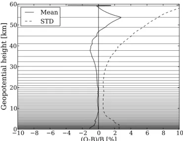
If the “reference” refractivity, including the moist term, is evaluated at intermediate “pseudo-levels” which lie between the model levels (having first calculated Eq. (11) on these pseudo-levels, ensuring continuity of the pressure), then the exponential assumption can be accurately applied between these levels (if there are sufficient additional levels), so the current (exponential) operator can simply be invoked mul-tiple times within each model layer. For future changes, this is a flexible approach as the computation only needs to evaluate the refractivities on the pseudo-levels and the Abel integral remains unchanged, hence additional assump-tions/simplifications can be avoided and a more sophisticated form could potentially be used. The number of pseudo-levels must be chosen to provide a balance between accuracy and computational cost. It has been found that using just one ad-ditional pseudo-level in the middle of each layer gives a good improvement for the associated cost. Two or more equally spaced pseudo-levels only provide very small improvements to the innovation statistics for the single pseudo-level case, so results with just one pseudo-level are presented here. For the layer in which the tangent point lies, the refractivity expres-sion, Eq. (10), is used to evaluateN at the tangent height, and at an additional pseudo-level halfway between the tan-gent point and the next highest model level. The resulting innovation statistics are shown in Fig. 8.
Figure 8.Bending angle innovation statistics, using hydrostatic re-fractivity (Eq. 10, including the moisture term) evaluated on one additional pseudo-level per model layer, and using an exponential function of refractivity with height to evaluate the Abel integral be-tween the model/pseudo-levels.
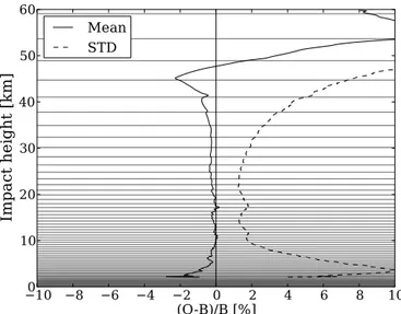
tangent height and the next model level as was described above. The motivation for investigating this is to explain why the innovations from the L91 ECMWF system (ECMWF, 2007) do not show these oscillations as strongly as in the L70 Met Office (Davies et al., 2005) statistics. At a height of 35 km, where the oscillations in the bias are prominent, the level spacing of the L91 ECMWF model is∼1.5 km, and at the Met Office (L70) it is∼2.9 km, i.e. a factor of∼2 differ-ent. Figure 9 shows the innovations when pseudo-levels are used in this configuration.
By comparing Figs. 9 and 3, it can be seen that by dou-bling the effective number of levels, the oscillations are re-duced, and hence this provides an explanation as to why the ECMWF statistics do not display these features as strongly. In other words, the exponential assumption is more accept-able with the L91 resolution, but less so for L70.
Similarly, when the ECMWF levels are thinned by a fac-tor of two, the innovation statistics show the oscillafac-tory bias much more strongly, and is very similar to the Met Office bias structure. This is shown in Figs. 10 and 11. The ECMWF im-plementation used in these plots is described in Appendix A3 and uses a 12 km cut-off, below which the original operator is used.
Another contributing factor to the smaller oscillatory bias using ECMWF profiles is that the ECMWF height levels are more variable in this region than the Met Office levels and this could lead to the smoothing out of the oscillatory signal, but this effect has not been investigated here.
For reasons of longer-term flexibility and maintenance, this approach is due to be implemented at the Met Of-fice in 2014, whereas the expansion of the dry refractivity
Figure 9. Bending angle innovation statistics, using hydrostatic refractivity (Eq. 10, including the moisture term) evaluated on a doubled-resolution vertical grid and using an exponential function of refractivity with height to evaluate the Abel integral between the model/pseudo-levels
Figure 10. Bending angle innovation statistics from the 91-level ECMWF model, using observations from all RO instruments over a 30-day period (April 2013). Typical model level heights are over-laid. The statistics generated using the original “ROPP” operator are plotted in black, and the ECMWF implementation of the improved operator is plotted in grey (see Appendix A3 for full details).
Figure 11. Bending angle innovation statistics as per Fig. 10, but with the background profiles thinned to half the vertical resolution of the 91-level ECMWF model.
4 Conclusions
It has been demonstrated that when the vertical model level spacing is large, the assumption of exponentially varying refractivity leads to systematic negative biases in forward-modelled stratospheric refractivities and bending angles for which the magnitudes are largest when the observation height lies between the model levels. The use of a more phys-ical form of refractivity as a function of height has been in-vestigated. This function assumes exponentially varying hu-midity, linearly varying temperature and hydrostatic pres-sure. Using this function, the magnitude of the oscillatory bias has been reduced considerably in both refractivity and bending angle statistics using Met Office background pro-files. Three approaches to implement such an improvement have been suggested:
1. integrate an approximation to the dry-hydrostatic tivity analytically above a point where the moist refrac-tivity term is negligible;
2. apply a polynomial correction to the exponential to make it a better approximation to the hydrostatic form; 3. evaluate the hydrostatic refractivity on mid-layer
pseudo-levels and use the exponential function in the Abel integral between the model/pseudo-levels. These methods each have their own merits, and these have been stated in the text.
In Appendix A, two methods of approximating the dry hydrostatic form are given and the resulting bending angle statistics are consistent.
Appendix A: Semi-analytical methods of evaluating the Abel integral for non-exponentialN (x)
A1 Form ofN (x)to be integrated
Between two model levelsiandi+1, we currently assume
N (x)=Nie−ki(x−xi), (A1)
where
ki =
ln(Ni/Ni+1)
xi+1−xi
. (A2)
It would be desirable to use the form of N (x) given in Eq. (18), which guarantees continuity of N and obeys the hydrostatic equation, but this will not allow the Abel inte-gral to be evaluated analytically, so a different approach is required. We achieve this by approximating the dry hydro-static refractivity, N (x), as the exponential form multiplied by an appropriate polynomial factor,K(x):
N (x)=Nie−ki(x−xi)K(x). (A3)
To exactly reproduce the adjusted dry hydrostatic form (with the correction,σ to force continuity),Kmust take the form:
K(x)=eki(x−xi)
1+βi(x−xi) Ti
−σi Rg −1
. (A4)
Simplifying the notation with X=x−xi and γi=
g
σiR+1
:
K(x)=ekiX
1+βiX
Ti
−γi
. (A5)
A series expansion of this factor about X=0 gives the following up to the quadratic term:
K(x)≃1+
−βTiγi
i +
k
X+ (A6)
1 2
βi2γi(γi+1)
Ti2 −
2βiγik
Ti +
k2 !
X2.
Although this is an expansion of a continuous function, the truncation of the series will produce small discontinuities. Therefore, we again enforce continuity as follows:
K(x)≃1+
−βTiγi
i +
k
X (A7)
− 1 Xi+1
−βiγi
Ti +
k
X2,
whereXi+1=xi+1−xi.
The form of the refractivity is then
N (x)=Nie−k(x−xi) (A8)
h
1+C1(x−xi)+C2(x−xi)2
i ,
where
C1 =
−βTiγi
i +
k
(A9)
C2 =
1
xi+1−xi
−βiγi
Ti +
k
.
A2 Evaluating the integral
With a few steps, this form of the refractivity with height can be inserted into the Abel integral. First, ln(n)is calculated: ln(n)≃n−1=10−6N=10−6Nie−k(x−xi)× (A10)
h
1+C1(x−xi)+C2(x−xi)2
i
so the numerator in the integrand of the Abel transform is d ln(n)
dx =10
−6N
iek(xi−a)e−k(x−a)× (A11)
h
P1+P2(x−a)+P3(x−a)2 i
,
where the following coefficients have been found by express-ing the polynomial factor in terms of(x−a)
P1 = C1−k−(2C2−C1k) (xi−a)−kC2(xi−a)2
P2 = 2C2−C1k+2kC2(xi−a)
P3 = −kC2.
By assuming that√x2−a2≃√2a√x−a (this is most accurate close to the tangent point), the contribution to the bending angle from a single model layer is given by integrat-ing the above in Eq. (7):
1α= −10−6√2a ek(xi−a)× (A12)
erfnpk (x−a)o√π
P
1
k1/2+
P2 2k3/2+
3P3 4k5/2
+
√
x−a e−k(x−a)
−P2
k +
P3(−2k (x−a)−3) 2k2
xi+1
xi
.
A3 Alternative approach
A slightly different approach can be used to obtain d lnn/dx
Starting with the equation for dry refractivity without the adjustment for continuity (Eq. 17), the refractivity gradient with height is
dN
dx = −
g
RT (x)+ β T (x)
N (x) (A13)
= −k(x)N (x),
where N (x) is the refractivity at x, and T (x)=Ti+
β (x−xi). Here,β=dT (x)/dx.
We currently assume a fixedkthroughout the layer, com-puted as in Eq. (A2). Call thiskmand assume that this value
is valid at the centre of the model layerxm=(xi+xi+1) /2. From Eq. (A13), k is inversely proportional to tempera-ture:
k=A
T, (A14)
whereAis just a constant. So, dk
dT = − k
T (A15)
in the layer. The change inkcan be written as
δk = −k
TδT (A16)
= −k T [β δx].
We can therefore approximate the variation ofkwithin the layer as
k(x)≃km−
kmβ
Tm
(x−xm) . (A17)
We then compute the refractivity expression for thisk(x): Z dN
N = −
Z
km−
kmβ
Tm
(x−xm)
dx (A18)
so,
ln(N )= −
km(x−xi)−
kmβ
2Tm
(x−xm)2−c
, (A19)
wherecis a constant of integration. To get appropriate values atxi andxi+1
N (x)= (A20)
Niexp
−km(x−xi)+
kmβ
2Tm
(x−xm)2−d
,
whered is chosen to ensure the refractivity is continuous at the model levels; thus,
d=(xi−xm)2=(xi+1−xm)2. (A21)
If the second term in the exponential is small then we can approximate
N (x)=Niexp(−km(x−xi))× (A22)
1+kmβ
2Tm
(x−xm)2−d
.
This makes the largest change to the pure exponential at the centre of the layer. Note that the sign of the temperature gradient determines the sign of the correction. Therefore, in the stratosphere, whereβ >0, the forward-modelled refrac-tivity will be underestimated without the correction, which is consistent with the oscillatory bias present in Fig. 2. The vertical gradient of ln(n)is
d lnn
dx ≃10
−6N
iexp(−ki(x−xi))× (A23)
−ki−
k2iβ
2Tm
(x−xm)2−d
+kTiβ
m
(x−xm)
! ,
which can be cast into the same form as Eq. (A11), using the coefficients:
P1= −ki−
k2iβ
2Tm
(a−xm)2−d
+kTiβ
m
(a−xm)
P2= −
ki2β Tm
(a−xm)+
kiβ
Tm
(A24)
P3= −
ki2β
2Tm
.
Note that ifβ=0, P1= −ki andP2=P3=0, so as ex-pected, we return to the original equation.
Appendix B: Impact of discontinuity in vertical refractivity gradients on bending angle
The question of whether it is necessary or desirable for dN/dx to be continuous has implications for bending an-glesαcalculated from refractivitiesNby means of the Abel transform (definingN=n−1 in this Appendix to avoid the usual factors of 10−6in the equations that follow)
α(a) = −2a
∞ Z
a
dN/dx √
x2−a2dx (B1)
≈ −√2a
∞ Z
a
dN/dx √
x−adx.
Consider the effect of a discontinuity inN′=dN/dx at
x=x0. This may be caused, for instance, by a rapid change in temperature gradient, such as occurs at the tropopause. For, in a dry atmosphere (cf. Eq. A13),
dN
so that a sudden change in dT /dx would cause a jump in dN/dx. Note that we assume thatN itself is continuous ev-erywhere, and that dN/dxis finite everywhere.
B1 In particular To be specific, we assume
N (x)=
N0exp(−k1(x−x0)) ifx≥x0
N0exp(−k0(x−x0)) ifx < x0 , (B3) whereN0=N (x0)andk1> k0(>0)for definiteness (cor-responding to a more positive dT /dx above x0 in the “tropopause” model above).
This implies dN/dx=
−k1N0exp(−k1(x−x0)) ifx≥x0
−k0N0exp(−k0(x−x0)) ifx < x0
, (B4)
so that there is a jump in dN/dxof magnitude|k1−k0|N0at
x0.
Substitution of Eq. (B4) into Eq. (B1) shows that, ifa≥ x0,
α(a)=p2π ak1N0exp(−k1(a−x0)) (B5)
and ifa < x0,
α(a)= (B6)
p
2π ak0N0exp(−k0(a−x0))erf( p
k0(x0−a))+ p
2π ak1N0exp(−k1(a−x0))erfc( p
k1(x0−a)).
The key point is that the bending angle is continuous atx0:
α(x0+)=α(x0−)=√2π x0k1N0. A secondary point is that the same cannot be said for the derivative of α – indeed, dα/da (x0−)is formally infinite. In fact, forajust belowx0, Eq. (B6) implies
α(a)−α(x0)=2 p
2x0(x0−a)N0(k0−k1)+O(x0−a). (B7) Note thatα(a) < α(x0)whenk1> k0. This is because the
(x−a)−1/2factor in Eq. (B1) means thatα(a)is dominated by the contribution fromN′just belowx0, which in this case is smaller (in magnitude) thanN′just above it.
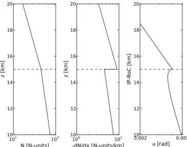
Figure B1 shows N, dN/dx and α for a 15 km “tropopause”.k0=0.1 km−1;k1=0.2 km−1. The continuity ofαatx0=15 km is clear, as is its cusp just below. The re-fractivity at the “tropopause” is 45 N-units, and the radius of curvature used in the bending angle calculation is 6350 km. B2 In general
More generally, suppose that there is a jump in dN/dxatx0. Is the bending angle continuous there?
The singular “kernel”(x−a)−1/2in Eq. (B1) complicates matters, so we assume initially that dN/dx varies smoothly fromN−′ =N′(x0−δ0)toN+′ =N′(x0+δ1). (Recall that we
Figure B1.Example profiles of (from left to right)N,−dN/dxand αwhen there is a discontinuity in dN/dxatx0=15 km. (For this plot,N=106(n−1)as usual.
assume it remains finite throughout.) We examine the differ-ence betweenα(x0−δ0)andα(x0+δ1)asδ0andδ1tend to 0 independently. Equation (B1) implies
α(x0−δ0) = − p
2(x0−δ0) ∞ Z
x0−δ0
N′(x) √
x−x0+δ0
dx (B8)
= −p2(x0−δ0)
x0+δ1 Z
x0−δ0
N′(x) √
x−x0+δ0 dx−
p
2(x0−δ0) ∞ Z
x0+δ1
N′(x) √
x−x0+δ0
dx, (B9)
while
α(x0+δ1)= − p
2(x0+δ1) ∞ Z
x0+δ1
N′(x) √
x−x0−δ1
dx. (B10)
Hence the difference in bending angle across the disconti-nuity atx0is given by
α(x0−δ0)−α(x0+δ1)=
−p2(x0−δ0)
x0+δ1 Z
x0−δ0
N′(x) √
x−x0+δ0
dx (B11)
−
∞ Z
x0+δ1
√
2(x0−δ0)
√
x−x0+δ0−
√
2(x0+δ1)
√
x−x0−δ1
Firstly, p
2(x0−δ0)
x0+δ1 Z
x0−δ0
N′(x) √
x−x0+δ0 dx ≤ p
2(x0−δ0)2 p
δ0+δ1 max
−δ0≤x−x0≤δ1|
N′(x)|. (B12) Secondly, ∞ Z
x0+δ1
√
2(x0−δ0)
√
x−x0+δ0−
√
2(x0+δ1)
√
x−x0−δ1
N′(x)dx = 2 ∞ Z 0 p
2(x0+δ1)N′(u2+x0+δ1)du−
2 ∞ Z
√
δ0+δ1 p
2(x0−δ0)N′(u2+x0−δ0)du ≤ 2 √
δ0+δ1 Z
0 p
2(x0+δ1)N′(u2+x0+δ1)du + 2 ∞ Z √
δ0+δ1
[p2(x0+δ1)N′(u2+x0+δ1)−
p
2(x0−δ0)N′(u2+x0−δ0)]du
. (B13)
The first of these last two integrals satisfies 2 √
δ0+δ1 Z
0 p
2(x0+δ1)N′(u2+x0+δ1)du ≤ p
2(x0+δ1)2 p
δ0+δ1 max
δ1≤x−x0≤δ0+2δ1
|N′(x)|. (B14) The second integral is first order inδ0andδ1. Formally,
2 ∞ Z
√
δ0+δ1
[p2(x0+δ1)N′(u2+x0+δ1)− (B15)
p
2(x0−δ0)N′(u2+x0−δ0)]du =2 p
2x0(δ0+δ1)× ∞
Z
√
δ0+δ1
[N′(u2+x0)/2x0+N′′(u2+x0)+O(δ02, δ 2 1)]du.
This final integral is almost certainly bounded asδ0, δ1→ 0; it certainly is ifN′andN′′decay with height faster than exp(−κx)for someκ >0, as is likely to be the case in prac-tice. Moreover, it is hard to think of a realistic refractivity profile that would cause the integral to diverge at least as fast as(δ0+δ1)−1asδ0, δ1→0. Hence, with this weak proviso, Eqs. (B11), (B12), (B14) and (B15) imply
|α(x0−δ0)−α(x0+δ1)| ≤ (B16) p
2(x0−δ0)2 p
δ0+δ1 max −δ0≤x−x0≤δ1|
N′(x)|+
p
2(x0+δ1)2 p
δ0+δ1 max
δ1≤x−x0≤δ0+2δ1|
N′(x)|+
O(δ0+δ1),
which tends to zero asδ0andδ1tend to 0. Hence the bending angle is continuous atx0.
As an example, if we just assume a linear ramp in N′
between N−′ =N′(x0−δ) to N+′ =N′(x0+δ), and (dif-ferent) exponential declines above and below x0, as in Sect. B1, and calculate the resulting bending angles by very high-resolution numerical evaluation of the Abel integral in Eq. (B1), then we find thatα(x0+δ)−α(x0)∝δ, and that
α(x0−δ)−α(x0)∝
√
δ, so that overall the difference in the bending angles betweenx0−δandx0+δgoes as
√
δ, as pre-dicted by Eq. (B16), and from which the continuity ofαat
Acknowledgements. This work was carried out as part of EUMET-SAT’s Radio Occultation Meteorology Satellite Application Facil-ity (ROM SAF) which is a decentralised operational RO processing centre under EUMETSAT.
We acknowledge Taiwan’s National Space Organization (NSPO) and the University Corporation for Atmospheric Research (UCAR) for providing the data and data products from the COSMIC/FORMOSAT-3 mission. We also acknowledge EUMET-SAT and the ROM SAF for providing Metop-A and Metop-B GRAS data and also to GFZ for providing data from TerraSAR-X and GRACE-A.
Also, thanks to Bruce Ingleby and Tim Payne (Met Office) for useful discussions.
Edited by: A. K. Steiner
References
Abramowitz, M. and Stegun, I. A. (Eds.): Handbook of mathemati-cal functions, Dover, 1965.
Cucurull, L., Derber, J. C., and Purser, R. J.: A bending angle for-ward operator for global positioning system radio occultation measurements, J. Geophys. Res. Atmo., 118, 14–28, 2013. Davies, T., Cullen, M. J. P., Malcolm, A. J., Mawson, M. H.,
Stani-forth, A., White, A. A., and Wood, N.: A new dynamical core for the Met Offices global and regional modelling of the atmosphere, Q. J. Roy. Meteorol. Soc., 131, 1759–1782, 2005.
ECMWF: IFS Documentation – Cy38r1. Part III: Dynamics and nu-merical procedures, IFS documentation, ECMWF, available at: https://software.ecmwf.int/wiki/display/OIFS/Documentation/ (last access: 3 October 2014), 2007.
Fjeldbo, G., Kliore, G. A., and Eshleman, V. R.: The neutral atmo-sphere of Venus as studied with the Mariner V radio occultation experiments, Astron. J., 76, 123–140, 1971.
Healy, S. B.: Assimilation of GPS radio occultation measurements at ECMWF, in: Proceedings of GRAS SAF Workshop on Appli-cations of GPS radio occultation measurements, ECMWF, Read-ing, 99–109, 2008.
Healy, S. B. and Eyre, J. R.: Retrieving temperature, water vapor and surface pressure information from refractive–index profiles derived by radio occultation: A simulation study, Q. J. Roy. Me-teorol. Soc., 126, 1661–1683, 2000.
Healy, S. B. and Thepaut, J.-N.: Assimilation experiments with CHAMP GPS radio occultation measurements, Q. J. Roy. Me-teorol. Soc., 132, 605–623, 2006.
Kursinski, E. R., Hajj, G. A., Schofield, J. T., Linfield, R. P., and Hardy, K. R.: Observing earth’s atmosphere with radio occulta-tion measurements using the Global Posiocculta-tioning System, J. Geo-phys. Res., 102, 23429–23465, 1997.
Melbourne, W. G., Davis, E. S., Duncan, C. B., Hajj, G. A., Hardy, K. R., Kursinski, E. R., Meehan, T. K., and Young, L. E.: The application of spaceborne GPS to atmospheric limb sounding and global change monitoring, Publication 94–18, Jet Propulsion Laboratory, Pasadena, Calif., 1994.
Poli, P., Healy, S. B., and Dee, D. P.: Assimilation of Global Po-sitioning System radio occultation data in the ECMWF ERA-Interim reanalysis, Q. J. Roy. Meteorol. Soc., 136, 1972–1990, 2010.
Rennie, M. P.: The impact of GPS radio occultation assimilation at the Met Office, Q. J. Roy. Meteorol. Soc., 136, 116–131, 2010. Smith, E. K. and Weintraub, S.: The constants in the equation for