Carbon monoxide climatology derived from the trajectory mapping of global MOZAIC-IAGOS data

(1)

ACPD

15, 29871–29937, 2015

Trajectory-mapped MOZAIC-IAGOS CO

climatology

M. Osman et al.

Title Page

Abstract Introduction

Conclusions References

Tables Figures

◭ ◮

Back Close

Full Screen / Esc

Printer-friendly Version Interactive Discussion

Discussion

P

a

per

|

Discussion

P

a

per

|

Discussion

P

a

per

|

Discussion

P

a

per

|

Atmos. Chem. Phys. Discuss., 15, 29871–29937, 2015 www.atmos-chem-phys-discuss.net/15/29871/2015/ doi:10.5194/acpd-15-29871-2015

This discussion paper is/has been under review for the journal Atmospheric Chemistry and Physics (ACP). Please refer to the corresponding final paper in ACP if available.

Carbon monoxide climatology derived

from the trajectory mapping of global

MOZAIC-IAGOS data

M. Osman1, D. W. Tarasick1, J. Liu2, O. Moeini1, V. Thouret3, V. E. Fioletov1, M. Parrington4, and P. Nédélec3

1

Environment Canada, 4905 Du_fferin Street, Downsview, ON, M3H 5T4, Canada

2

Department of Geography and Program in Planning, University of Toronto, 100 St. George Street, Toronto, Ontario, M5S 3G3, Canada

3

Laboratoire d’Aérologie, UMR5560, CNRS and Université de Toulouse, Toulouse, France

4

European Centre for Medium-Range Weather Forecasts, Shinfield Park, Reading, RG2 9AX, UK

Received: 17 September 2015 – Accepted: 12 October 2015 – Published: 2 November 2015

Correspondence to: D. W. Tarasick (david.tarasick@ec.gc.ca)

Published by Copernicus Publications on behalf of the European Geosciences Union.

(2)

ACPD

15, 29871–29937, 2015

climatology

M. Osman et al.

Title Page

Tables Figures

◭ ◮

Back Close

Full Screen / Esc

Discussion

P

a

per

|

Discussion

P

a

per

|

Discussion

P

a

per

|

Discussion

P

a

per

|

Abstract

A three-dimensional gridded climatology of carbon monoxide (CO) has been developed by trajectory mapping of global MOZAIC-IAGOS in situ measurements from commer-cial aircraft data. CO measurements made during aircraft ascent and descent, compris-ing nearly 41 200 profiles at 148 airports worldwide from December 2001 to December

5

2012 are used. Forward and backward trajectories are calculated from meteorological reanalysis data in order to map the CO measurements to other locations, and so to fill in the spatial domain. This domain-filling technique employs 15 800 000 calculated tra-jectories to map otherwise sparse MOZAIC-IAGOS data into a quasi-global field. The resulting trajectory-mapped CO dataset is archived monthly from 2001–2012 on a grid

10

of 5◦longitude×5◦latitude×1 km altitude, from the surface to 14 km altitude.

The mapping product has been carefully evaluated, by comparing maps constructed using only forward trajectories and using only backward trajectories. The two meth-ods show similar global CO distribution patterns. The magnitude of their differences is most commonly 10 % or less, and found to be less than 30 % for almost all cases. The

15

trajectory-mapped CO dataset has also been validated by comparison profiles for indi-vidual airports with those produced by the mapping method when data from that site are excluded. While there are larger differences below 2 km, the two methods agree very well between 2 and 10 km with the magnitude of biases within 20 %.

Maps are also compared with Version 6 data from the Measurements Of

Pollu-20

tion In The Troposphere (MOPITT) satellite instrument. While agreement is good in the lowermost troposphere, the MOPITT CO profile shows negative biases of∼20 % between 500 and 300 hPa. These upper troposphere biases are not related to the mapping procedure, as almost identical differences are found with the original in situ MOZAIC-IAGOS data. The total CO trajectory-mapped MOZAIC-IAGOS climatology

25

(3)

ACPD

15, 29871–29937, 2015

climatology

M. Osman et al.

Title Page

Tables Figures

◭ ◮

Back Close

Full Screen / Esc

Discussion

P

a

per

|

Discussion

P

a

per

|

Discussion

P

a

per

|

Discussion

P

a

per

|

The maps clearly show major regional CO sources such as biomass burning in the central and southern Africa and anthropogenic emissions in eastern China. The dataset shows the seasonal CO cycle over different latitude bands and altitude ranges that are representative of the regions as well as long-term trends over latitude bands. We observe a decline in CO over the Northern Hemisphere extratropics and the tropics

5

consistent with that reported by previous studies.

Similar maps have been made using the concurrent O₃measurements by MOZAIC-IAGOS, as the global variation of O3–CO correlations can be a useful tool for the

eval-uation of ozone sources and transport in chemical transport models. We anticipate use of the trajectory-mapped MOZAIC-IAGOS CO dataset as an a priori climatology for

10

satellite retrieval, and for air quality model validation and initialization.

1 Introduction

Atmospheric carbon monoxide (CO) is an important global air pollutant and trace gas. Due to its relatively long lifetime of 1–4 months (Hubler et al., 1992; Law and Pyle, 1993), it is an ideal tracer for long range atmospheric transport (Logan et al., 1981;

15

Lelieveld et al., 2001; Shindell et al., 2006). Moreover, in the tropics, it is an important tracer of upward transport during convective events (e.g., Pommrich et al., 2014). Con-sequently, it has been employed to facilitate interpretations of chemical measurements (Jaffe et al., 1996; Parrish et al., 1991, 1998; Wang et al., 1996, 1997) and in validating chemical transport models (Carmichael et al., 2003; Liu et al., 2003; Tan et al., 2004;

20

Wang et al., 2004). The main sources of atmospheric CO are relatively well under-stood (Galanter et al., 2000; Granier et al., 2011; Holloway et al., 2000); however, the magnitude of individual sources and their seasonal variability, especially of biomass burning, are not well quantified. Stein et al. (2014) also reported that models are also generally biased low due to either an underestimation of CO sources or an

overesti-25

mation of its sinks. There are di_fferences in the emission densities of anthropogenic and natural sources, despite the fact that the anthropogenic and natural sources are

(4)

ACPD

15, 29871–29937, 2015

climatology

M. Osman et al.

Title Page

Tables Figures

◭ ◮

Back Close

Full Screen / Esc

Discussion

P

a

per

|

Discussion

P

a

per

|

Discussion

P

a

per

|

Discussion

P

a

per

|

of similar magnitude on a global scale (Granier et al., 2011; Logan et al., 1981). The anthropogenic sources are primarily associated with large industrial centers or ma-jor biomass burning regions while the natural sources, such as oxidation of methane (CH₄) and non-methane hydrocarbons (NMHCs) are much more diffuse. This makes CO a good atmospheric tracer gas for anthropogenic emissions as its lifetime allows

5

it to be used as an indicator of how large-scale atmospheric transport redistributes pollutants on a global scale.

CO plays a vital role in the chemistry of the atmosphere. This significance mainly comes from the influence of CO on the concentrations and distributions of the atmo-spheric oxidants, ozone (O₃), the hydroperoxy (HO₂) and hydroxyl radicals (OH) (e.g.

10

Novelli et al., 1994, 1998). Reaction (R1) between CO and OH represents 90–95 % of the CO sink (Logan et al., 1981), and about 75 % of the removal of OH (Thompson, 1992) in the troposphere:

CO+OH → CO2+H (R1)

H+O2 → HO2+M (R2)

15

In areas with sufficient NO_x (=NO+NO₂), HO₂formed in Reaction (R2) leads to pho-tochemical Reactions (R3)–(R5) which bring about net O3production. In urban areas

and regions of biomass burning, large amounts of these O3 precursors will be

pro-duced, and O₃ can be formed in, and downwind of, the source region (Crutzen, 1973; Fishman and Seiler, 1983):

20

HO₂+NO → OH+NO2 (R3)

NO2+hν → NO+O(<425 nm) (R4)

O2+O+M → O3 (R5)

O3 is associated with respiratory problems and decreased crop yields (e.g., McKee,

1993; Chameides et al., 1994). Since CO and OH are principal reaction partners, CO

25

(5)

ACPD

15, 29871–29937, 2015

climatology

M. Osman et al.

Title Page

Tables Figures

◭ ◮

Back Close

Full Screen / Esc

Discussion

P

a

per

|

Discussion

P

a

per

|

Discussion

P

a

per

|

Discussion

P

a

per

|

organic compounds in the atmosphere. Via these interactions with OH, O₃ and CH₄, CO has an indirect radiative forcing of about 0.25 W m−2(IPCC AR5).

Global atmospheric chemistry models require accurate CO concentrations on a global scale in order to define spatial and temporal variations of atmospheric oxidants and CO. For this reason measurements of CO are made by different kinds of remote

5

sensing and in situ instruments, in ground-based networks, aircraft programmes and from space (Novelli et al., 1994, 1998; Rinsland and Levine, 1985; Zander et al., 1989; Brook et al., 2014; Reichle et al., 1990, 1999; Worden et al., 2013; Petzold et al., 2015). Background CO levels are found in all regions of the troposphere, where mixing ratios between 45 and 250 ppbv have been reported (Novelli et al., 1994). Extreme mixing

10

ratios much higher than 250 ppb have been observed in the upper troposphere over Asia (Nédélec et al., 2005) or over the Pacific (Clark et al., 2015) in plumes of boreal biomass burning. The largest values in the lower troposphere have been observed over Beijing (Zbinden et al., 2013).

Early studies of ground-based observations showed increasing trends in global CO

15

before 1980 (Khalil and Rasmussen, 1988; Rinsland and Levine, 1985; Zander et al., 1989), followed by a modest decline in the 1990s (Novelli et al., 1994, 2003; Khalil and Rasmussen, 1994). More recently satellite observations have shown that the de-cline has continued: Worden et al. (2013) report a global trend from 2000–2011 of ∼10 % decade−1 on column CO in the Northern Hemisphere. Petetin et al. (2015)

20

show a similar decrease of about 2 ppb year−1 over Frankfurt throughout the tropo-sphere from 2002 to 2012. The decrease is at least partly due to a decrease in global anthropogenic CO emissions (Granier et al., 2011).

In-service Aircraft for a Global Observing System (IAGOS), and its predecessor Mea-surement of OZone and water vapor by AIrbus in-service airCraft (MOZAIC), have

25

been making automatic and regular measurements of O₃, water vapour and stan-dard meteorological parameters onboard long-range commercial Airbus A340 aircraft since August 1994 (Marenco et al., 1998; Petzold et al., 2015). Measurements of CO (Nédélec et al., 2003) and NO_y (Volz-Thomas et al., 2005) were added in late 2001.

(6)

ACPD

15, 29871–29937, 2015

climatology

M. Osman et al.

Title Page

Tables Figures

◭ ◮

Back Close

Full Screen / Esc

Discussion

P

a

per

|

Discussion

P

a

per

|

Discussion

P

a

per

|

Discussion

P

a

per

|

The MOZAIC database currently contains data from more than 71 900 vertical profiles of O3and 41 200 vertical profiles of CO, measured during takeoffand landing from 148

airports around the world. MOZAIC measurements show the general features of the atmospheric CO distribution (Zbinden et al., 2013; Petzold et al., 2015 and references therein), capturing major regional features (e.g., strong CO emissions from biomass

5

burning or anthropogenic sources).

The objective of this paper is to present a three-dimensional (i.e., latitude, longi-tude, altitude) gridded climatology of carbon monoxide that has been developed by trajectory mapping of global MOZAIC-IAGOS CO data from 2001–2012. We employ a domain-filling technique, using approximately 15 800 000 calculated trajectories to

10

map otherwise sparse MOZAIC-IAGOS CO data into a global field.

This is a technique that has been used successfully with tropospheric and strato-spheric ozonesonde data (G. Liu et al., 2013; J. Liu et al., 2013). Stohl et al. (2001) used trajectory statistics to extend one year of MOZAIC O₃ measurements into a 4-season O3 climatology at 10◦ longitude by 6◦ latitude and three vertical heights.

Tara-15

sick et al. (2010) developed high resolution (1◦×1◦×1 km in latitude, longitude, and al-titude) tropospheric O₃fields for North America from ozonesonde data from the INTEX (Intercontinental Transport Experiment) and ARCTAS (Arctic Research of the Composi-tion of the Troposphere from Aircraft and Satellites) campaigns, and this was extended to global tropospheric ozonesonde data by G. Liu et al. (2013). It is possible to apply

20

this technique to CO because the lifetime of CO in the troposphere, as noted above, is generally of the order of weeks or months. This physically-based interpolation method, using the reanalysis meteorological data from the National Centers for Environmen-tal Prediction/National Center for Atmospheric Research (NCEP/NCAR) (Kalnay et al., 1996), offers obvious advantages over typical statistical interpolation methods. Indeed,

25

it is expected to improve global models and satellite data validation and it can also be used as a priori for satellite data retrieval.

(7)

ACPD

15, 29871–29937, 2015

climatology

M. Osman et al.

Title Page

Tables Figures

◭ ◮

Back Close

Full Screen / Esc

Discussion

P

a

per

|

Discussion

P

a

per

|

Discussion

P

a

per

|

Discussion

P

a

per

|

pollution. The 3-D global trajectory-mapped CO climatology facilitates visualization and comparison of different years, decades, and seasons, and offers insight into the global variation of CO. Moreover, it will be useful for climate and air quality model initializa-tion and validainitializa-tion, and can be used as an a priori climatology for satellite data re-trievals. Comparison with similar maps made using the concurrent O3 measurements

5

by MOZAIC-IAGOS allow us to examine the global variation of O3–CO correlations,

which convey information about the source distribution of CO.O₃–CO correlations are also of great interest around the tropopause region since such correlations provide in-formation on mixing processes (e.g., Hoor et al., 2004; Pan et al., 2006; Vogel et al., 2011) besides of the source regions. This paper is organized in the following order.

Fol-10

lowing discussion of the MOZAIC-IAGOS and MOPITT instruments in Sects. 2.1 and 2.2, respectively, we describe trajectory mapping calculation via HYSPLIT model in Sect. 2.3. The transformtion of MOZAIC-IAGOS data by applying the MOPITT a priori profile and averaging kernels is presented in Sect. 2.4. The validation of the trajectory-mapped dataset against MOZAIC-IAGOS in situ data will be presented in Sect. 3.

15

The same section assesses the differences between the CO mapping produced us-ing only backward and only forward trajectories, and also compares with in situ global CO data at cruise altitudes between 8 and 12 km. Subsequently, the comparison of the trajectory-mapped MOZAIC-IAGOS CO with MOPITT CO retrievals is presented in Sect. 4. Section 5 discusses the results obtained from the global 3-D trajectory-mapped

20

climatology data. After pointing out the potential applications of the trajectory-mapped MOZAIC-IAGOS CO climatology (i.e., O3–CO relationship and global variation and

trends of CO) in Sect. 6, we make concluding remarks about the results we obtain from this study in Sect. 7.

(8)

ACPD

15, 29871–29937, 2015

climatology

M. Osman et al.

Title Page

Tables Figures

◭ ◮

Back Close

Full Screen / Esc

Discussion

P

a

per

|

Discussion

P

a

per

|

Discussion

P

a

per

|

Discussion

P

a

per

|

2 Measurements of CO

2.1 MOZAIC-IAGOS

CO measurements were made by an improved version of a commercial Model 48CTL CO Analyzer from Thermo Environmental Instruments employing the Gas Filter Corre-lation technique. The Model 48CTL is based on the principle that CO absorbs infrared

5

radiation at a wavelength of 4.67 microns. For 30 s integration time (the response time of the instrument) the precision achieved is 5 ppb (noise) or 5 % (calibration) CO, with minimum detection limit of 10 ppb. The analyzer samples at a horizontal resolution of about 7 km (since the maximum cruise speed of the Airbus A340 aircraft is nearly 250 m s−1) and the vertical resolution during ascents and descents is nearly 300 m.

10

Nedelec et al. (2003 for MOZAIC, 2015 for IAGOS) give detailed descriptions of the CO analyzer, measurement technique, instrument validation and quality testing.

The airports visited by aircraft equipped with MOZAIC-IAGOS instrumentation are shown in Fig. 1. Further details are available at http://www.iagos.fr.

The sampled data from these airports are unevenly distributed both spatially and

15

temporally because the frequency of visits to airports by aircraft that take part in MOZAIC-IAGOS varies considerably depending on commercial airlines’ operational constraints. This means that at airports such as Frankfurt, Germany we find as many as 12 324 CO profiles while from Dammam, Saudi Arabia we have only 2 CO profiles during the period 2001–2012. The trajectory-mapping method is valuable for filling the

20

sparse and variable spatial domain.

2.2 MOPITT

MOPITT is a nadir-viewing gas correlation radiometer which provides global atmo-spheric profiles of CO volume mixing ratio (VMR) and CO total column values using near-infrared radiation at 2.3 µm and thermal-infrared radiation at 4.7 µm. CO columns

25

(9)

ACPD

15, 29871–29937, 2015

climatology

M. Osman et al.

Title Page

Tables Figures

◭ ◮

Back Close

Full Screen / Esc

Discussion

P

a

per

|

Discussion

P

a

per

|

Discussion

P

a

per

|

Discussion

P

a

per

|

scenes. The MOPITT measurement technique relies on thermal contrast between the Earth’s surface and atmosphere, leading to a retrieval dependence on surface tem-perature, and little sensitivity to CO in the boundary layer. The retrieval uses a priori profiles that vary geographically and temporally. MOPITT-derived CO VMR profiles re-flect the vertical sensitivity of the measurement as defined by the retrieval averaging

5

kernel (e.g. Fig. 2) and a priori profile. In this study, we have used Level 3, Version 6 monthly CO mixing ratio profile data, reported on 10 pressure levels, as well as CO to-tal column. MOPITT data are publicly available at the NASA Langley Research Center Atmospheric Science Data Center: https://eosweb.larc.nasa.gov/project/mopitt/mopitt_ table.

10

MOPITT was launched in 1999 into sun-synchronous polar orbit with a 1030 lo-cal time (LT) northward or southward lolo-cal equator cross-over time. The instrument field of view is 22 km×22 km. Cross-track scanning with a 612 km swath provides near complete coverage of the surface of the Earth approximately every 3 days. MOPITT retrievals have gone through intensive validation against in situ measurements from

15

aircraft on a regular basis since the start of the mission (Worden et al., 2010; Deeter et al., 2012, 2013, 2014; Emmons et al., 2004, 2007, 2009; Jacob et al., 2003). MO-PITT CO retrievals have also been validated by comparing to ground-based and TES satellite measurements (Jacob et al., 2003 and Lou et al., 2007). In the lower tropo-sphere a mean positive bias of 6–8 % against in situ validation profiles has been

re-20

ported, and a mean bias and standard deviation for the retrieved CO column of 5±11 and−0.5±12.1 % for periods, respectively, March 2000–May 2001 and August 2001– December 2002 (Emmons et al., 2004). Jacob et al. (2003) reported the CO bias to be 6±2 %, where as Emmons et al. (2007) found approximately 7±8 % bias for summer 2004 measurements. Deeter et al. (2013) also show a total column retrieval bias of

25

about 0.08×1018molecules cm−2(∼4 %) against in situ profiles. Furthermore, Deeter et al. (2012) reported a positive bias of surface-level CO concentrations on the order of a few percent against in situ profiles.

(10)

ACPD

15, 29871–29937, 2015

climatology

M. Osman et al.

Title Page

Tables Figures

◭ ◮

Back Close

Full Screen / Esc

Discussion

P

a

per

|

Discussion

P

a

per

|

Discussion

P

a

per

|

Discussion

P

a

per

|

2.3 Trajectory calculation and global CO mapping via HYSPLIT

For each CO profile of the MOZAIC-IAGOS data set presented here, the mean CO VMR was calculated for 1 km intervals from sea level up to 12 km (the maximum alti-tude of the aircraft). Cruise data were not used. The HYSPLIT (Hybrid Single-Particle Lagrangian Integrated Trajectory) model version 4.9 (Draxler and Hess, 1998; Draxler,

5

1999) was employed to calculate trajectories for each level of each profile. HYSPLIT, publicly accessible at (http://ready.arl.noaa.gov/HYSPLIT.php), uses the reanalysis me-teorological wind fields from the National Centers for Environmental Prediction/National Center for Atmospheric Research (NCEP/NCAR) (Kalnay et al., 1996) as an input to describe the transport of CO in the atmosphere. The reanalysis data are readily

avail-10

able from 1948 until the present. Both forward and backward trajectories for 4 days at 6 h intervals (32 positions for each level) were calculated for 41 200 CO profiles, and the mean CO mixing ratios from each level (i.e., tropospheric and lower stratospheric air masses) of each profile were assigned to the corresponding trajectory positions along the forward and backward paths. Trajectories only move upward and downward

15

with the meteorological vertical velocity fields since the HYSPLIT kinematic trajectory model employs vertical motions supplied with the NCEP reanalysis meteorological data set. Numerous studies show that the choice of vertical wind velocity has significant im-pact on the transport of tracers (e.g., Schoeberl et al., 2003; Ploeger et al., 2010, 2012). Kinematic models show excessive dispersion for tracers with strong gradients

20

(e.g., O3in the vicinity of the tropopause), particularly for trajectories of 7 days or more.

We limit trajectories to a maximum for 4 days in length. Moreover, unlike O₃, CO does not have strong vertical gradient in the upper troposphere. Trajectories that reach the bottom boundary (i.e., ground) continue at the surface where the trajectory robust-ness grows to be more uncertain. Trajectories that reach the top height of the model

25

(11)

ex-ACPD

15, 29871–29937, 2015

climatology

M. Osman et al.

Title Page

Tables Figures

◭ ◮

Back Close

Full Screen / Esc

Discussion

P

a

per

|

Discussion

P

a

per

|

Discussion

P

a

per

|

Discussion

P

a

per

|

ception of Frankfurt where we can get up to 6 profiles day−1. In this trajectory-mapped MOZAIC-IAGOS CO climatology, we did not exclude major anthropogenic CO sources; however, the climatology could in principle be refined by excluding backtrajectories from sources identified via emission inventories. We note, however, that if major an-thropogenic sources were a significant source of error, we would see differences

be-5

tween the CO mapping produced using only backward and only forward trajectories (see Sect. 3.1).

This mapping implicitly assumes that CO chemistry may be neglected over a timescale of 4 days. Except near major anthropogenic sources, this assumption should be valid, as the lifetime of CO is much longer. However, trajectories have

sig-10

nificant errors over such timescales. Stohl (1998) in a comprehensive review, quotes typical errors of about 100–200 km day−1_{in the troposphere. This can be combined with} an estimate of the correlation length in the troposphere to yield an estimate for the infor-mation value of a mapped measurement. Liu et al. (2009) find that O3measurements

in the troposphere correlate with an exponential dependence of approximatelye−r1.5

15

(withr shown in Eq. 1), and a correlation length of 500–1000 km in the troposphere, and 1000–2000 km in the stratosphere. The means that the horizontal distance for the correlation coefficient to decrease by a factor ofeis 500–1000 km in the troposphere and 1000–2000 km in the stratosphere. As the CO lifetime is even longer than the ozone lifetime, the correlation length for CO should be at least as large. Therefore, the

20

trajectory-mapped data were binned at intervals of 5◦_{latitude and 5}◦_{longitude, at every} 1 km altitude, and averaged with a weighting,w, assigned according to the formula:

w=e−(150t/R)1.5 ₍₁₎

where R is the correlation length (700 and 1500 km in the troposphere and strato-sphere, respectively), andtis the age of the trajectory in days.

25

The trajectory mapping greatly spreads out the in situ CO information along the tra-jectory paths, increasing the spatial domain to include much of the globe. Two different vertical coordinate systems were utilized for the binning, and hence the maps were

(12)

ACPD

15, 29871–29937, 2015

climatology

M. Osman et al.

Title Page

Tables Figures

◭ ◮

Back Close

Full Screen / Esc

Discussion

P

a

per

|

Discussion

P

a

per

|

Discussion

P

a

per

|

Discussion

P

a

per

|

generated for elevations above sea level and above ground level. Data are available publicly at ftp://es-ee.tor.ec.gc.ca/pub/ftpdt/. In this work, we present global CO maps generated for elevations above sea level. Global maps of monthly, annual, seasonal and decadal means are presented, for each altitude, from 2001–2012.

2.4 MOZAIC-IAGOS Comparison with MOPITT

5

When comparing the MOPITT retrievals with in situ data, it is necessary to take into account the sensitivity of the retrievals to the true profiles. The method used by MOPITT to retrieve tropospheric CO profiles follows that of Rodgers (2000). In order to perform the most meaningful and accurate comparison, the in situ data to be compared must be transformed using the averaging kernel matrix,A, and a priori profile, xa, as shown by

10

Eq. (2). A “retrieved” comparison profile,xret, is calculated by using the in situ profile,x,

as the “true” profile in Eq. (2) which is interpolated to the lower resolution of MOPITT. As described by Emmons et al. (2004), the in situ profile (x) is transformed with averaging kernel matrix (A) and the a priori CO profile (xa) to get a profile (xret), the appropriate

quantity to compare with the MOPITT retrievals:

15

xret=xa+A(x−xa)=Ax+(I−A)xa (2)

whereIis the identity matrix. The averaging kernels provide the relative weighting be-tween the true and a priori profiles and reflect the sensitivity of the retrieval to the measurement. They are very sensitive to the surface temperature and will be different for each point on the globe. The matrixAdescribes the sensitivity of the retrieved CO

20

log(VMR) profile to perturbations applied at each level of the “true” log(VMR) profile. The quantityxret, the transformed in situ profile, represents the result of applying a

lin-ear transformation to the in-situ profile in the same way that the remote sensing retrieval process is believed to transform the true profile. Thus,xret can be directly compared

against the MOPITT retrieved CO profile in a manner that is not affected by varying

ver-25

tical resolution or a priori dependence.xret,x, andxaare expressed in terms of the

(13)

ACPD

15, 29871–29937, 2015

climatology

M. Osman et al.

Title Page

Tables Figures

◭ ◮

Back Close

Full Screen / Esc

Discussion

P

a

per

|

Discussion

P

a

per

|

Discussion

P

a

per

|

Discussion

P

a

per

|

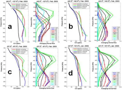
The vertical resolution of the retrieved profile is described by the shapes of the av-eraging kernels. Figure 2 shows that the kernels are broad except at pressure levels between 400–300 hPa and exhibit a large degree of overlap. The overlap of the aver-aging kernels peaking in the boundary layer and those at the top of the atmosphere indicates a significant correlation for the retrieved values at these levels. The retrieved

5

CO values at these levels are also influenced by CO at mid levels, and by the a priori CO profile at all pressure levels. The averaging kernels describe the relative contri-butions, to the CO VMR retrieved at a given level, of the true and a priori (via I₋A) CO profiles at all pressure levels (Eq. 2). Where the area under the averaging kernel is smaller, the a priori information in the retrieved CO profile is relatively larger.

MO-10

PITT CO averaging kernels exhibit variability from month to month, season to season as well as nighttime to daytime, depending on the atmospheric temperature profile, surface pressure and the CO profile itself.

The vertical coordinate of the MOZAIC-IAGOS climatology profile is km a.s.l., while the MOPITT a priori profile and averaging kernels are on pressure levels in hPa.

There-15

fore, before applying the MOPITT averaging kernels the climatology data were interpo-lated using NCEP global pressure profiles that vary as a function of time (month) and latitude, to the 10 vertical pressure grid levels (1000, 900, 800, 700, 600, 500, 400, 300, 200, and 100 hPa) used by MOPITT. The interpolated profile was then convolved with the a priori profile and the averaging kernels following Eq. (2) (Emmons et al., 2004).

20

For the atmospheric residual above the maximum MOZAIC-IAGOS profile altitude, the MOPITT a priori profiles were used.

In order to compare with these transformed CO profiles, the MOPITT CO profiles, averaging kernels, and a priori profiles were mapped down from the original hori-zontal resolution of 1◦×1◦ in latitude and longitude to a reduced 5◦×5◦ grid. The

25

mapping was linear in log pressure and volume mixing ratio of CO. An example of comparisons of trajectory-mapped MOZAIC-IAGOS CO profiles with an individual (re-duced) 5◦×5◦ MOPITT CO profiles is shown in Fig. 2. The original trajectory-mapped MOZAIC-IAGOS CO profile, the a priori profile, and the transformed trajectory-mapped

(14)

ACPD

15, 29871–29937, 2015

climatology

M. Osman et al.

Title Page

Tables Figures

◭ ◮

Back Close

Full Screen / Esc

Discussion

P

a

per

|

Discussion

P

a

per

|

Discussion

P

a

per

|

Discussion

P

a

per

|

MOZAIC-IAGOS CO profile are shown along with the MOPITT retrieved CO profile. The application of the averaging kernels to the MOZAIC-IAGOS CO profile results in significant vertical transformation, which can shift mixing ratios significantly at some levels. The averaging kernel, for example, identified as “1000” (i.e., surface) shows how changes to the true CO mixing ratio at all ten retrieval levels would each

con-5

tribute to a change in the retrieved value at the surface at 1000 mbar. The original trajectory-mapped MOZAIC-IAGOS climatology profile is quite different from the trans-formed climatology profile and as seen from the same figure the departures of the transformed CO mixing ratio from the true mixing ratios can be as large as 60 ppb at some pressure levels.

10

3 Validation

Validation of the trajectory-mapped MOZAIC-IAGOS CO dataset product has been per-formed by Eq. (1) comparing maps constructed using only forward trajectories against with those constructed using only backward trajectories, and Eq. (2) comparing pro-files for individual airports against those produced by the mapping method when data

15

from that site are excluded. The airport stations that have been selected in this valida-tion study represent tropical and Northern Hemisphere midlatitude locavalida-tions that are subject to different meteorological and CO source conditions.

3.1 Comparison of trajectory-mapped MOZAIC-IAGOS CO profiles

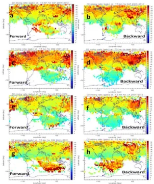
As a first step in validation of the trajectory-mapped climatology, Figs. 3 and S1 (in

20

the Supplement) assess the differences between the CO mapping produced using only backward and only forward trajectories for different seasons using the 7.5 km level as an example. If chemistry (i.e. local sources or sinks) were a significant source of error then one would expect to see differences between these maps. In fact, the CO distribution patterns are very similar (Fig. 3). Differences are most commonly 10 % or less, and

(15)

ACPD

15, 29871–29937, 2015

climatology

M. Osman et al.

Title Page

Tables Figures

◭ ◮

Back Close

Full Screen / Esc

Discussion

P

a

per

|

Discussion

P

a

per

|

Discussion

P

a

per

|

Discussion

P

a

per

|

found to be less than 30 % for almost all cases. They are typically less than 10 % at northern mid-latitudes and less than 20 % in the tropics between±30◦latitude, except in the Pacific and Atlantic oceans where they can be as large as 30 %. As Fig. S1 illustrates, differences also show no distinct pattern, except for some clustering in areas where the trajectories are longest, and therefore least reliable. As differences between

5

the two distributions are comparable with the uncertainties of the mean value estimates and not systematic, it is reasonable to combine forward and backward mapped values to produce an averaged CO map.

3.2 Comparison between trajectory-mapped and in situ profiles

A good test of an interpolation model is to examine how it performs in areas where

10

no data are available. Figure 4 compares the trajectory-mapped climatology profiles at three airport sites (Frankfurt, Germany; Houston, USA; and Tokyo, Japan) with the average of the MOZAIC-IAGOS data from each of these sites for May of 2001–2012. However, since the sampling frequency varies from airport to airport, Houston and Tokyo are not as well sampled as Frankfurt throughout the period. The climatology

15

profiles for each location were produced by excluding data from that location, but using all other MOZAIC-IAGOS data.

Generally, the profiles from the two methods agree very well and the agreement is especially good in the free troposphere, at altitudes between 2 and 10 km. Referring to the bottom panels of Fig. 4, the magnitude of the differences for most altitudes is well

20

under 20 %.

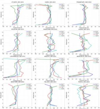
In Fig. 5 we extend the comparisons shown in Fig. 4 for other seasons as well as for another airports that represent different meteorological and source conditions. The se-lected airports are Atlanta (USA), Cairo (Egypt), Frankfurt (Germany), Houston (USA), Khartoum (Sudan), Lagos (Nigeria), Los Angeles (USA), Nagoya (Japan), New Delhi

25

(India), New York (USA), Tel Aviv (Israel) and Tokyo (Japan). Again, the sampling fre-quency among the airports is not the same throughout the period. Similar to the results shown in Fig. 4, in Fig. 5 we notice good agreement between the trajectory-mapped

(16)

ACPD

15, 29871–29937, 2015

climatology

M. Osman et al.

Title Page

Tables Figures

◭ ◮

Back Close

Full Screen / Esc

Discussion

P

a

per

|

Discussion

P

a

per

|

Discussion

P

a

per

|

Discussion

P

a

per

|

and the in situ measurements for different locations and seasons across the globe. There are larger differences below 2 km where trajectories have larger errors predomi-nantly due to complex dispersion and turbulence in the planetary boundary layer (Stohl and Seibert, 1998). However, the overall agreement between 2 and 10 km is very good with biases again within 20 %. As in previous studies using this method, the largest

5

differences are seen where other sources of data are distant. The smallest overall bias is seen at Frankfurt, even though the exclusion of Frankfurt data removes nearly 1/3 of the total number of profiles. Apparently data from nearby airports such as Munich (Germany) and Brussels (Belgium) map accurately to the Frankfurt location. The con-sistency of these validation tests suggests that the trajectory-mapped dataset provides

10

a reliable picture of the tropospheric CO distribution.

3.3 Comparison with the MOZAIC-IAGOS in-situ for upper troposphere

We can also compare the trajectory-mapped profile data and MOZAIC-IAGOS in situ global CO data at cruise altitudes between 8 and 12 km. The maps found at http: //www.iagos.fr/macc/reanalysis_climatology_CO.php show the global seasonal mean

15

(December–February, March–May, June–August and September–November) distribu-tion of CO in the upper troposphere (within 60 hPa below the tropopause) for the period from 2003 to 2011. The figure clearly shows the seasonal cycle of CO with seasonal maximum in the Northern Hemisphere (NH) spring (MAM) and peak CO values in the Southern Hemisphere (SH) spring (SON). Elevated CO levels in the upper troposphere

20

are generally seen over the areas where there is strong biomass burning. The figure also reveals high CO emissions are observed over eastern China in MAM primarily due to a rise in coal use (Boden et al., 2009; Gregg et al., 2008; Tie et al., 2006) and a increasing number of vehicles (Cai and Xie, 2007).

Figure 6 shows the trajectory-mapped global seasonal variation of CO for

25

(17)

ACPD

15, 29871–29937, 2015

climatology

M. Osman et al.

Title Page

Tables Figures

◭ ◮

Back Close

Full Screen / Esc

Discussion

P

a

per

|

Discussion

P

a

per

|

Discussion

P

a

per

|

Discussion

P

a

per

|

However, major regional features of the global CO distributions for different seasons are clearly evident in both figures. The figures show seasonal high CO values in spring in both hemispheres and elevated CO levels over regions where there is in-tensive biomass burning (central Africa, southern Africa and South America) and an-thropogenic emissions (eastern China). Comparable CO values are noticeable from

5

the figures over the Northern Atlantic Ocean as well as Greenland. Such an overall good qualitative agreement between the trajectory-mapped CO and MOZAIC-IAGOS in situ CO cruise data result suggests that the trajectory-mapped CO dataset performs well in remote areas as well.

4 Trajectory-mapped MOZAIC-IAGOS Versus MOPITT

10

This section is devoted to comparing the trajectory-mapped MOZAIC-IAGOS CO dataset with the extensively validated product from the MOPITT instrument onboard the NASA Terra satellite, which has been operating continuously since March 2000 (Drummond and Mand, 1996; Edwards et al., 1999). Global comparison was made for both CO profiles and CO total column for different time periods.

15

4.1 Comparison with MOPITT CO profiles

As described in Sect. 2.4, in order to make a rigorous comparison with MOPITT data, the climatology profiles are first transformed using the corresponding MOPITT a priori profiles and averaging kernels via Eq. (2). Figure 2 shows examples of retrieved CO profiles (xret), together with the original climatology (x) and the a priori profiles (xa).

20

When examining the comparison between the MOPITT CO retrieval and the trajectory-mapped CO profile it is useful to keep in mind the shapes of the averag-ing kernels. For example, the 100 and 1000 mbar kernels are typically less peaked than the other pressure levels. Consequently, the generally broad and weak averaging kernel demonstrates that a significant fraction of the information used in the retrieval is

25

(18)

ACPD

15, 29871–29937, 2015

climatology

M. Osman et al.

Title Page

Tables Figures

◭ ◮

Back Close

Full Screen / Esc

Discussion

P

a

per

|

Discussion

P

a

per

|

Discussion

P

a

per

|

Discussion

P

a

per

|

from the a priori profile or CO from other layers or both. Figure 2 also cautions that the transformed trajectory-mapped MOZAIC-IAGOS CO is closer to both the MOPITT CO retrievals and a priori profiles when there is less information from the measurement. Furthermore, as can be seen from Fig. 2, the MOPITT retrievals are not able to resolve the finer scale vertical structure of the trajectory-mapped CO profiles. The departures

5

of the retrieved CO VMR from the trajectory-mapped VMRs at some pressure levels are as large as 60 ppb. In the lower troposphere the MOPITT CO retrieval profile is positively biased whereas the bias is negative in the upper troposphere. In Fig. 2, we have used only the dayside retrievals from MOPITT as the dayside retrievals have the maximum information content (Deeter et al., 2004). The MOPITT V6 L3 retrievals are

10

used in this analysis.

Figure 7 shows profile comparisons between MOPITT retrievals and the MOZAIC-IAGOS climatology for global CO data at pressure levels 900, 700, 500, and 300 hPa. The slopes and correlations between MOPITT CO retrievals and the CO climatology (after applying the averaging kernels and the a priori profiles) for different levels are

in-15

dicated in the figure. The different dot colors shown in Fig. 7 stand for different latitude bands: 23.5–66.5◦_{S (SH extratropics), 23.5}◦_S–23.5◦_{N (tropics), 23.5–66.5}◦_{N (NH} ex-tratropics). The same figure shows that there are clearly two distinct clusters of dots in Fig. 7a and b and the high CO VMRs values seen here are from tropics with a very few from the NH extratropics. The enhanced CO values may have originated from

an-20

thropogenic sources and/or biomass burning; however, identifying individual sources is beyond the scope of this paper. Recent work by Ding et al. (2015) shows the asso-ciation of enhanced CO in the free troposphere with the uplifting of CO from biomass burning and anthropogenic sources.

MOPITT and trajectory-mapped MOZAIC-IAGOS CO climatology mixing ratios are

25

(19)

ACPD

15, 29871–29937, 2015

climatology

M. Osman et al.

Title Page

Tables Figures

◭ ◮

Back Close

Full Screen / Esc

Discussion

P

a

per

|

Discussion

P

a

per

|

Discussion

P

a

per

|

Discussion

P

a

per

|

Although in Fig. 7 we have chosen to show biases for January 2001–2012, the same analysis for other months and time periods yields similar results.

MOPITT seems to underestimate CO VMR by as much as 21 % against the trajectory-mapped MOZAIC-IAGOS CO climatology at 500 hPa. This result is signifi-cantly different from previous work such as Deeter et al. (2014, 2013, 2010) and

Em-5

mons et al. (2004, 2007, 2009). Most of these examined earlier versions of the MOPITT L3 product, although Deeter et al. (2014) use the MOPITT L3 V6 product, and reported biases varying from −5.2 % at 400 hPa to 8.9 % at the surface. In all cases the vali-dation data consisted of flask samples taken by NOAA aircraft. In order to eliminate the possibility that trajectory errors might be contributing to the bias we find with the

10

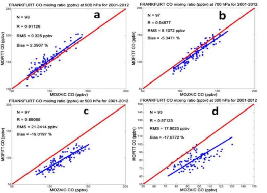
MOZAIC-IAGOS CO dataset, we have also compared MOZAIC-IAGOS in situ CO pro-files against MOPITT retrievals. As an example in Fig. 8, we display the comparison between MOZAIC-IAGOS in situ CO profiles at Frankfurt (Germany) and MOPITT CO retrievals over Frankfurt from MOPITT overpasses. The MOZAIC-IAGOS in situ aircraft CO values have been transformed using the MOPITT averaging kernels and a priori

15

data, for the period from December 2001–December 2012. MOPITT and MOZAIC-IAGOS are again strongly correlated, and biases at 500 and 300 hPa are large, and in fact very similar in magnitude to those with respect to the trajectory-mapped MOZAIC-IAGOS CO dataset.

A global comparison between the trajectory-mapped MOZAIC-IAGOS climatology

20

and MOPITT at 600 hPa is displayed in Fig. 9. As can be seen from the same figure both datasets capture major features of the CO distribution, particularly anthropogeni-cally polluted (i.e., northeast China) and biomass burning (i.e., west Africa, central Africa, South Africa and central America) regions. The CO-rich air in the lower tropo-sphere over west Africa, where biomass burning fires are active, is convectively lifted

25

vertically upward to the upper troposphere where it disperses over the African tropics towards the east coast of South America and the south Arabian peninsula (Edwards et al., 2003). In this region, higher CO VMRs are measured by MOZAIC-IAGOS than MOPITT. Over southeast Asia, MOZAIC-IAGOS detects highly polluted air-masses. In

(20)

ACPD

15, 29871–29937, 2015

climatology

M. Osman et al.

Title Page

Tables Figures

◭ ◮

Back Close

Full Screen / Esc

Discussion

P

a

per

|

Discussion

P

a

per

|

Discussion

P

a

per

|

Discussion

P

a

per

|

these areas MOZAIC-IAGOS also measures higher CO than MOPITT. Comparison of the panels for DJF with those for SON of Fig. 9 also show that the NH CO VMRs are much higher during December–February than September–November (a result of the difference in OH, as noted above) and the latitude gradient in December–February is higher than in September–November. This is because in the SH the seasonal peak

5

in CO occurs in September–November. This comparison also reveals a shift of the biomass burning from central Africa to South Africa and central America. Both datasets capture this, although the TIR/NIR product offers the greatest sensitivity to CO in the lower troposphere (Deeter et al., 2014). MOZAIC-IAGOS shows higher CO concentra-tions in these regions than MOPITT. On the other hand, Liu et al. (2005) suggested

10

that since MOPITT (V3 L2) has low sensitivity to CO in the lower troposphere, the CO VMR estimated may only be a lower bound. The same authors noted that fires can be missed if not large enough or if they do not coincide with the MOPITT overpass time, or both. The presence of clouds is also another limitation for missing data.

Figure S2 shows global maps of percentage differences between MOPITT and the

15

transformed trajectory-mapped MOZAIC-IAGOS CO climatology at 800 and 600 hPa pressure levels for DJF and SON 2001–2012. Di_fferences are generally less than ±20 % at 800 hPa, with a negligible overall bias, but larger at 600 hPa, with MOPITT on average 10–20 % higher except few places over the Caribbean, southeast Asia and central Africa. Generally, the comparisons of the CO profiles of the transformed

20

trajectory-mapped MOZAIC-IAGOS and MOPITT for both grid cells as well as zonal mean for different latitude bands show a consistent, significant bias: MOPITT is lower from about 700 to 300 hPa, but shows a negligible bias in the lowermost troposphere. Above 300 hPa, they seem to agree better, although this may be partly due to the fact that the retrieved CO values in this region are highly influenced by the MOPITT a priori

25

(21)

ACPD

15, 29871–29937, 2015

climatology

M. Osman et al.

Title Page

Tables Figures

◭ ◮

Back Close

Full Screen / Esc

Discussion

P

a

per

|

Discussion

P

a

per

|

Discussion

P

a

per

|

Discussion

P

a

per

|

4.2 Comparison with MOPITT CO total column values

CO total column amounts are retrieved from the MOPITT observations in addition to the profile retrievals. The retrieved CO total columncret(a scalar) is related to the retrieved

profilexret(a vector) through the linear relation

cret=tTxret (3)

5

where T indicates the transpose operation andt is the total column vectors. The CO total column averaging kernel can be calculated from the profile averaging kernels by

a=tTA (4)

The column operator simply converts the mixing ratio for each retrieval level to a partial column amount. Using the hydrostatic relation, the operatortis expressed as

10

t₌2.120×1013∆p (5)

Equation (5) is expressed in molecules cm−2_ppbv−1_and _∆_p_{is the vector of the} thick-nesses of the retrieval pressure levels (in hPa). The interfaces of the retrieval layers are set at the surface, top of the atmosphere, and the midpoints between the standard nine retrieval levels. Determination of ∆p required in Eq. (5) has to be made individually

15

for each retrieval because of the variability of the surface pressure. The boundaries of the imaginary layer associated with each level are located at the pressure midpoints between the levels in the grid.

For example, for a surface pressure of 950 hPa, the fixed retrieval pressure grid lev-els along with surface pressure would be (950, 900, 800, 700, 600, 500, 400, 300,

20

200, 100) hPa. Hence the corresponding∆p values would be (25, 75, 100, 100, 100, 100, 100, 100, 100, 100) hPa. Column amounts are calculated from the in situ profiles according to Eq. (6) to validate the CO total column retrievals.

In the same manner as we have done for the retrieved CO profiles, the retrievals of CO total columncretmay be compared against total column values derived from in situ

25

(22)

ACPD

15, 29871–29937, 2015

climatology

M. Osman et al.

Title Page

Tables Figures

◭ ◮

Back Close

Full Screen / Esc

Discussion

P

a

per

|

Discussion

P

a

per

|

Discussion

P

a

per

|

Discussion

P

a

per

|

profilesx. Utilizing Eq. (2), the retrievals of the total CO column cret found in Eq. (3)

can be rewritten alternatively as

cret=ca+a(x−xa) (6)

whereca=t T

xa is the a priori total column value corresponding to the a priori profile

xa,ais the CO total column averaging kernel andx is the in situ profile.

5

We have calculated the global total CO columns for both the MOZAIC-IAGOS CO cli-matology (using the MOPITT a priori and averaging kernels by applying Eq. 6) and for MOPITT CO retrievals and compared different regions of the globe and different times from 2001–2012. The comparisons between the climatology and the MOPITT obser-vations agree well, typically to within 10 %. For most regions the MOPITT CO total

10

columns are slightly higher than the trajectory-mapped MOZAIC-IAGOS CO climatol-ogy total columns while in high CO source regions MOPITT seems to underestimate CO emissions. The SH shows a distinct latitude gradient, which not evident in the NH. This is likely related to the existence of major CO sources in the NH and the absence of large sources of emission in the SH. Nighttime CO observations of MOPITT have

15

not been validated and appear subject to larger bias (Heald et al., 2004). Hence, we use the daytime data for comparison.

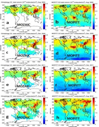
Figure 10 shows total column CO for August 2002, December 2005, December 2011 and August 2012. From Fig. 10, it is clear that MOPITT and the climatology are simi-larly able to capture the CO spatial variability. In August 2002 and 2012, elevated total

20

column CO is seen over South America, southeast Asia and west African which is due primarily to agricultural biomass burning in the regions. In both months, we see high total column CO over southeast Asia and west Africa. High total column CO is also seen over eastern China, which is one of the major emission regions in the world. Northern hemispheric total columns are much higher than those in the Southern

Hemi-25

(23)

ACPD

15, 29871–29937, 2015

climatology

M. Osman et al.

Title Page

Tables Figures

◭ ◮

Back Close

Full Screen / Esc

Discussion

P

a

per

|

Discussion

P

a

per

|

Discussion

P

a

per

|

Discussion

P

a

per

|

total column retrievals are slightly higher than the trajectory-mapped MOZAIC-IAGOS CO climatology.

Figure S3 shows global difference plots for the CO maps shown Fig. 10. Biases gen-erally lie within±20 %, and the global mean bias between the MOPITT and MOZAIC-IAGOS CO climatology total columns is typically about 5 % or less. While overall bias

5

shows MOPITT to be higher, it is also evident that the trajectory-mapped MOZAIC-IAGOS climatology is typically higher near major sources (eastern China, west central Africa and western South America) as well as over some areas of the oceans where aircraft data are not available. The negative biases near major sources are probably due to the limited vertical resolution of MOPITT as previously noted.

10

Similar results are found for other years (Fig. 11). This figure shows scatter plots of retrieved MOPITT CO total columns against the transformed trajectory-mapped MOZAIC-IAGOS climatology for August 2008, December 2008, August 2012 and De-cember 2012. MOPITT and the trajectory-mapped climatology generally show strong correlations, and average biases of less than 5 %. MOPITT is higher most cases. This

15

is consistent with previous work, which also shows positive total column retrieval bias against aircraft data (Deeter et al., 2014, 2013; Emmons et al., 2009, 2007).

5 Results

5.1 Global distribution of MOZAIC-IAGOS CO climatology

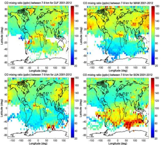
As an example, Fig. 12 shows the monthly mean CO VMR between 4 and 8 km

al-20

titude a.s.l. for the four seasons (i.e., December–February, March–May, June–August and September–November) during 2001–2012. The climatology is able to capture the CO spatial variability fairly well: the northern hemispheric concentrations are much higher, and the biomass burning peaks are clearly visible for the NH winter and spring seasons. The climatology shows more abundant CO in the NH during these seasons.

25

This is due primarily to lower OH levels during the cold season which permits a longer

(24)

ACPD

15, 29871–29937, 2015

climatology

M. Osman et al.

Title Page

Tables Figures

◭ ◮

Back Close

Full Screen / Esc

Discussion

P

a

per

|

Discussion

P

a

per

|

Discussion

P

a

per

|

Discussion

P

a

per

|

lifetime for CO, although there also appears to be an additional source in eastern Asia. Enhanced CO concentration is observed in the tropical regions where wildfire burning is typical during the December–February season, like west Africa and a large part of central Africa (Sauvage et al., 2005, 2007). At southern mid-latitudes between south-ern Africa and Australia, we observe high CO from September to November, during the

5

agricultural burning season. This is accompanied by enhanced ozone in the same re-gion (e.g. Ding et al., 2015; see also Sect. 5.2), produced via Reactions (R1)–(R5) and similar. Although Fig. 12 shows a 12-year global map, the strong enhanced CO over these regions (west Africa, South America, and southeast Asia) is clearly observable as an annual feature with significant interannual variability.

10

Furthermore, Fig. 12 allows us to examine the annual variation of the global distri-bution of CO between 4 and 8 km altitudes a.s.l. Despite the limited MOZAIC-IAGOS data in the SH, the seasonal cycle of CO is clearly shown in both hemispheres. The greatest change of CO from north to south occurs around the tropics in February–April when CO levels are greatest in the NH. The reverse gradient appears with a sharp

15

decrease across the tropics in September–October when CO levels peak in the SH. High CO levels are seen in August between southeast Africa and southwest Australia, which is as a result of the long-range transport of CO produced from biomass burning in the tropical areas (i.e., southern Africa).

5.2 Zonal distribution of MOZAIC-IAGOS CO climatology

20

5.2.1 Seasonal variation

In Fig. 13, data are grouped in three bands representing the NH extratropics (Fig. 13c), the SH extratropics (Fig. 13d), the tropics (Fig. 13b) and for latitude band 45◦_S–45◦_N (Fig. 13a). The zonal mean trajectory-mapped MOZAIC-IAGOS CO climatology for these latitude bands is shown for the altitude ranges 0–2, 2–4, 4–8 and 8–12 km.

25

(25)

ACPD

15, 29871–29937, 2015

climatology

M. Osman et al.

Title Page

Tables Figures

◭ ◮

Back Close

Full Screen / Esc

Discussion

P

a

per

|

Discussion

P

a

per

|

Discussion

P

a

per

|

Discussion

P

a

per

|

April following a steady increase during fall and winter. This is followed by a rapid de-crease giving rise to the lowest CO levels in July–August. The seasonal decline of CO VMR in summer shows the typical seasonal pattern of CO in the NH driven by OH increase during this time (Yurganov et al., 2008; Novelli et al., 1998). In the SH extratropics (Fig. 13d), CO levels peak in September–October. This is consistent with

5

previous studies by Novelli et al. (1998). In the SH, the annual CO maximum is earlier at lower altitudes. Rinsland et al. (2002) suggested this phenomenon to be associated with the vertical and horizontal CO dispersion away from the biomass burning region in the tropics. Moreover, CO shows greater seasonal variability, particularly at higher altitudes, in the SH than in the NH. This can also be seen in Fig. 12. The seasonal CO

10

cycle in the tropics (Fig. 13b) and for latitude band 45◦_S–45◦_{N (Fig. 13a) both display} a July minimum, and a secondary maximum in October while the primary maximum is in late NH winter/early spring. This CO cycle in both hemispheres is controlled by seasonal variations of OH, as OH is the major CO sink (Logan et al., 1981; Bergam-aschi et al., 2000; Novelli et al., 1998) and the space–time distribution of its sources

15

(Novelli et al., 1998), in particular the biomass burning either in the Tropics (largest fires occur in austral Africa and South America in SON) or at boreal latitudes (largest fires in June–July–August), and anthropogenic sources at northern mid-latitudes.

Figure 14 shows zonal mean latitude-time cross-section plots of CO VMR at 2.5, 4.5, 6.5, 8.5, 10.5 and 12.5 km altitudes for the period 2001–2012. The latitude-time

20

cross-section shows the seasonal cycle of zonal mean CO for different altitudes, as seen in the previous figures, and also the variation of the interhemispheric CO VMR gradient throughout the year. The strongest interhemispheric gradient occurs in March, at low altitude, and the smallest gradients are seen in northern summer. The gradient in NH spring reverses at higher altitudes, and in NH fall where it is especially strong

25

at higher altitudes. Plots 14e, f also clearly show the weak seasonal cycle in the NH upper troposphere compared to that in the SH.

(26)

ACPD

15, 29871–29937, 2015

climatology

M. Osman et al.

Title Page

Tables Figures

◭ ◮

Back Close

Full Screen / Esc

Discussion

P

a

per

|

Discussion

P

a

per

|

Discussion

P

a

per

|

Discussion

P

a

per

|

5.2.2 Vertical distribution

Figure 15 illustrates the variation of CO with altitude for the seasons in which we ob-serve maximum CO levels in both the SH and NH (i.e., MAM and SON). The seasons demonstrate the greatest CO VMRs at lower altitude in both hemispheres. Even though CO declines with altitude in both hemispheres, it does so faster in the NH than the SH,

5

which results in a decrease in the strength of the interhemispheric gradient (SH to NH) with altitude. This result is consistent with Edwards et al. (2006) who suggested that in the absence of continued CO input from the source regions (i.e., biomass burning in southern Africa and South America), the aged CO is gradually distributed vertically throughout the troposphere in the SH. In fact, in regions where there is deep convection

10

this leads to an enhanced CO concentration in the upper troposphere, as can be seen on the right-hand side of Fig. 15 and in Fig. 16d. Moreover, Liu et al. (2006) showed large horizontal CO gradients in association with vertical and horizontal transport of air originated from different chemical signatures.

The zonal CO mean vertical profiles for February, April, July and September,

av-15

eraged for 2001–2012, are shown in Fig. 16. The results are displayed for latitude bands 23.5–66.5◦N (NH extratropics), 23.5–66.5◦S (SH extratropics) and 23.5◦ S-23.5◦N (tropics). The CO profiles show strong seasonal and latitudinal variability. The largest VMRs of CO occur at lower altitudes in the NH extratropics in February and April but the strong decline with altitude causes CO VMRs to be higher in the SH at

20

high altitudes than in the NH. In the SH in February, April, July and September, there is little variation of CO with altitude. This is due to the sampling of the lower most strato-sphere in the NH much more frequently than in the SH. The trajectory-mapped CO in the SH extratropics is mainly representative of the tropics unlike in the NH extratrop-ics where there are many CO measurements north of 40◦N. The altitude gradients are

25

(27)

ACPD

15, 29871–29937, 2015

climatology

M. Osman et al.

Title Page

Tables Figures

◭ ◮

Back Close

Full Screen / Esc

Discussion

P

a

per

|

Discussion

P

a

per

|

Discussion

P

a

per

|

Discussion

P

a

per

|

SH. In tropics, CO VMRs show rapid decrease with altitude in the lower troposphere but above approximately 4–5 km changes with altitude are minor.

6 Applications

6.1 Global variation and trends of CO

The smoothed time series of the NH extratropical zonal mean CO VMR at 900, 700,

5

500, and 300 hPa for the trajectory-mapped MOZAIC-IAGOS dataset 2001–2012 is shown in Fig. 17. For purposes of comparison we also show data from MOPITT and from the mapped MOZAIC-IAGOS dataset transformed with the MOPITT averaging kernals. Gaps in the figure occur whenever one data source is missing. The gaps in June–July 2001 and August–September 2009 were due to a cooler failure of the

MO-10

PITT instrument. MOZAIC-IAGOS began CO measurement in December 2001 and there were only partial data available in 2010 and 2011. The observations show an annual late winter or springtime peak in the NH extratropical zonal CO loading each year, in conjunction with low wintertime OH levels. The same interannual cycle of CO is captured by both trajectory-mapped MOZAIC-IAGOS (transformed and untransformed)

15

and MOPITT. They appear to track short-term changes equally well. However, while all show a modest decline in the lower troposphere particularity until about 2008–2009 (and then CO VMR seems to level off), in accordance with the trends found by Wor-den et al. (2013), in the upper troposphere MOPITT shows a modest increase, and a significant bias with respect to trajectory-mapped MOZAIC-IAGOS that decreases

20

with time. Although the untransformed trajectory-mapped MOZAIC-IAGOS CO values show a significant difference against the transformed at lower troposphere, they seem to agree well at higher levels. However, the untransformed trajectory-mapped MOZAIC-IAGOS shows higher CO levels compared to MOPITT CO retrievals for all levels.

Laken and Shahbaz (2014) found increasing CO trends over widespread regions of

25

South America, Mexico, central Africa, Greenland, the eastern Antarctic, and the entire