Quantifying local-scale dust emission from the Arabian Red Sea coastal plain

www.atmos-chem-phys.net/17/993/2017/ doi:10.5194/acp-17-993-2017

© Author(s) 2017. CC Attribution 3.0 License.

Quantifying local-scale dust emission from the Arabian

Red Sea coastal plain

Anatolii Anisimov1, Weichun Tao1,a, Georgiy Stenchikov1, Stoitchko Kalenderski1, P. Jish Prakash1, Zong-Liang Yang2, and Mingjie Shi2,b

1_{King Abdullah University of Science and Technology (KAUST), Physical Science and Engineering Division (PSE),}

Thuwal, 23955-6900, Saudi Arabia

2_{The University of Texas at Austin, Jackson School of Geosciences, Department of Geological Sciences,}

Austin, TX 78712, USA

a_{now at: Policy Research Center of Environment and Economy, Ministry of Environmental Protection,}

Beijing, 100029, People’s Republic of China

b_{now at: Jet Propulsion Laboratory, California Institute of Technology, 4800 Oak Grove Drive, Pasadena, CA 91109, USA} Correspondence to:Georgiy Stenchikov ([email protected])

Received: 11 August 2016 – Published in Atmos. Chem. Phys. Discuss.: 25 August 2016 Revised: 17 December 2016 – Accepted: 22 December 2016 – Published: 23 January 2017

Abstract.Dust plumes emitted from the narrow Arabian Red Sea coastal plain are often observed on satellite images and felt in local population centers. Despite its relatively small area, the coastal plain could be a significant dust source; how-ever, its effect is not well quantified as it is not well approxi-mated in global or even regional models. In addition, because of close proximity to the Red Sea, a significant amount of dust from the coastal areas could be deposited into the Red Sea and serve as a vital component of the nutrient balance of marine ecosystems.

In the current study, we apply the offline Community Land Model version 4 (CLM4) to better quantify dust emission from the coastal plain during the period of 2009–2011. We verify the spatial and temporal variability in model results us-ing independent weather station reports. We also compare the results with the MERRA Aerosol Reanalysis (MERRAero). We show that the best results are obtained with 1 km model spatial resolution and dust source function based on Meteosat Second Generation Spinning Enhanced Visible and InfraRed Imager (SEVIRI) measurements. We present the dust emis-sion spatial pattern, as well as estimates of seasonal and di-urnal variability in dust event frequency and intensity, and discuss the emission regime in the major dust generation hot spot areas. We demonstrate the contrasting seasonal dust cy-cles in the northern and southern parts of the coastal plain and

discuss the physical mechanisms responsible for dust gener-ation.

This study provides the first estimates of the fine-scale spa-tial and temporal distribution of dust emissions from the Ara-bian Red Sea coastal plain constrained by MERRAero and short-term WRF-Chem simulations. The estimate of total dust emission from the coastal plain, tuned to fit emissions in MERRAero, is 7.5±0.5 Mt a−1. Small interannual variabil-ity indicates that the study area is a stable dust source. The mineralogical composition analysis shows that the coastal plain generates around 76±5 kt of iron oxides and 6±0.4 kt of phosphorus annually. Over 65 % of dust is emitted from the northern part of the coastal plain.

1 Introduction

The exploration of dust generation and transport, as well as climatology and seasonality of the dust cycle in the Ara-bian Peninsula, has been gaining increased attention in re-cent years (Hamidi et al., 2013, 2014; Kalenderski and Stenchikov, 2016; Kalenderski et al., 2013; Notaro et al., 2013, 2015; Prakash et al., 2015; Rezazadeh et al., 2013; Shalaby et al., 2015; Shi et al., 2016; Yu et al., 2013, 2015; Alobaidi et al., 2016). Along with a strong climate effect, dust outbreaks in this region affect the nutrient balance of the semi-enclosed Red and Arabian seas. For example, it was shown that the passage of major dust storms over the Arabian Sea causes chlorophyll blooming (Singh et al., 2008). The Red Sea, bordered by the Sahara and Arabian deserts, and with little or no river discharge and infrequent flash floods from land, is highly oligotrophic, especially in the northern part, rendering nutrients coming from the Indian Ocean al-most unobtainable (Acker et al., 2008; Chase et al., 2011; Weikert, 1987). Therefore, atmospheric dust and gaseous de-positions are especially important as nutrient supplies for the Red Sea (Kalenderski et al., 2013; Prakash et al., 2015).

Although previous studies indicate that dust outbreaks are most frequent over the eastern sector of Saudi Arabia (Barkan et al., 2004; Goudie and Middleton, 2006; Prospero et al., 2002; Shalaby et al., 2015; Washington et al., 2003), satellite images and ground observations show that there is a zone of increased dust activity in the western part of the Ara-bian Peninsula (Ackerman and Cox, 1989; Furman, 2003; Ginoux et al., 2012; Shao, 2008; Shao et al., 2011a; Walker et al., 2009; Yu et al., 2013). Located next to the Red Sea, the narrow coastal plain could make a significant contribution to the overall amount of dust depositing to the sea, trans-porting iron, phosphorus, and nitrogen. However, despite the importance of this source area for the nutrient balance of the Red Sea, no specific studies have been focused on the semidesert coastal region and no estimates of the amount of dust emitted from these areas have been made yet, partly due to the scarcity of observations and partly because the nar-row coastal plain is a subgrid area in most global and even regional modeling studies.

The concentration of dust particles in the atmosphere de-pends on small-scale emission processes, which are spatially heterogeneous and involve complex nonlinear interactions controlled by meteorological conditions and properties of land surfaces. As the measurement of emission in field con-ditions is extremely difficult, numerical models are the prin-cipal tools for dust emission evaluation. At the same time, the results from the AeroCom intercomparison project for atmo-spheric models that comprise aerosol components (Huneeus et al., 2011) suggest large discrepancies in model estimates of global dust emission and deposition by up to a factor of 10. As global models cannot approximate fine-scale circulations well, regional uncertainties in dust emissions are expected to be even higher. Due to the relatively small area and com-plex terrain structure of the western Arabian coastal plain, large-scale and even mesoscale models are not able to

repro-duce the dust emission processes here with the desired accu-racy. Even for similar meteorological conditions, a number of studies reported substantial differences in dust fluxes pre-dicted by different models, indicating the model deficiencies in accounting for fine-scale features such as soil texture and surface vegetation cover (Ginoux et al., 2012; Kang et al., 2011; Koven and Fung, 2008; Prospero et al., 2002; Shao, 2008; Textor et al., 2006; Todd et al., 2008; Zender et al., 2003b). Raupach and Lu (2004) identified key challenges in modeling wind erosion related to the representation of land-surface processes, including the fidelity of parameterizations and the availability of high-resolution input data for dust gen-eration calculations. Therefore, to obtain reliable estimates of dust emissions, especially in such highly heterogeneous re-gions as the Arabian Red Sea coastal plain, fine-resolution surface information is required.

Recently, satellite-derived high-resolution datasets of sur-face properties have emerged and provided an opportunity for improving dust emission calculations (Bullard et al., 2011; Ginoux et al., 2012; Kang et al., 2011; Knippertz and Todd, 2012; Pérez et al., 2011; Shao et al., 2011a). For ex-ample, Kim et al. (2013) and Hamidi et al. (2014), using a dynamic vegetation dataset, enabled a simple dust emission scheme to account for the control of seasonally varying vege-tation cover on dust emission, which is usually accounted for in more advanced schemes (Bullard et al., 2011; Mahowald et al., 2006; Zender et al., 2003a). Menut et al. (2013) re-ported that the State Soil Geographic Database (STATSGO-FAO), remapped from the Food and Agriculture Organiza-tion of the United NaOrganiza-tions (FAO) two-layer 5 min global soil texture dataset (Nickovic et al., 2012), provides realis-tic spatial patterns of dust emission for the Middle East and northern Africa. Shi et al. (2016) discussed the impact of the satellite-derived vegetation dataset on patterns and intensity of dust emission in the Arabian Peninsula. Many studies have been devoted to accurately locating dust source regions us-ing different criteria, accountus-ing for sediment availability and erodibility due to geographic influences, and applying satel-lite datasets to define so-called source functions (Ginoux et al., 2012; Kim et al., 2013; Parajuli et al., 2014; Walker et al., 2009; Zender et al., 2003b).

and apply the dust emission statistical source function and demonstrate the benefits of using high-resolution inventories. We compare the results with independent weather code and visibility reports from meteorological stations. Although these data are indirectly related to local dust emissions and cannot be applied for accurate model validation, they may provide valuable information and serve as a reference for determining optimal model configuration (Engelstaedter et al., 2006; Tegen, 2003). We also compare (and calibrate) our dust emission estimates with MERRA Aerosol Reanal-ysis (MERRAero) (Buchard et al., 2016), a recent reanalReanal-ysis product that includes an aerosol model component and has the highest spatial resolution compared with analogous prod-ucts, and with short-term Weather Research and Forecasting model coupled with Chemistry (WRF-Chem) simulations.

Marine productivity is largely limited by the availability of iron (Mahowald, 2009), which in turn depends on the solu-bility of iron-containing compounds in seawater. It has been shown that aerosol source mineralogy is a crucial factor for iron content and solubility as well as aging in the course of particle transport (Baker and Croot, 2010, and references therein). Together with iron, both phosphorus and nitrogen also frequently limit marine productivity (Okin et al., 2011). To evaluate the possible mineralogical composition of nutri-ents deposited in the Red Sea from local sources, we apply the global dataset of soil texture and mineral composition, GMINER30, developed by Nickovic et al. (2012). We as-sume that the mineral composition and size fractioning of the emitted dust are the same as those of the parent soil. This assumption does not always hold (Claquin et al., 1999; Perl-witz et al., 2015). Moreover, airborne dust changes its size distribution and mineralogical composition during its life cy-cle. Nevertheless, due to the short pathway from the coastal plain to the sea, the atmospheric processing of dust particles from this closely located source is less important compared to those subjected to long-range transport, and our assess-ment may serve as an initial estimate of the mineralogical composition of dust particles deposited to the Red Sea.

The rest of the article is organized as follows. In Sect. 2, we present the model description and characterize the study domain and observational datasets. In Sect. 3, we describe numerical experiments, examine model sensitivity to land-surface datasets, and compare results with station observa-tions. A detailed analysis of dust generation and its spatial-temporal variability is conducted in Sect. 4. We summarize our results and draw conclusions in Sect. 5.

2 Data and methods

2.1 CLM4 model and meteorological forcing

We perform the numerical experiments using the offline CLM4 (Lawrence et al., 2011; Oleson et al., 2010) im-plemented with the DEAD module (Zender et al., 2003a).

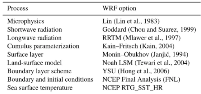
Table 1.WRF model configuration.

Process WRF option

Microphysics Lin (Lin et al., 1983)

Shortwave radiation Goddard (Chou and Suarez, 1999) Longwave radiation RRTM (Mlawer et al., 1997) Cumulus parameterization Kain–Fritsch (Kain, 2004) Surface layer Monin–Obukhov (Janji´c, 1994) Land-surface model Noah LSM (Tewari et al., 2004) Boundary layer scheme YSU (Hong et al., 2006) Boundary and initial conditions NCEP Final Analysis (FNL) Sea surface temperature NCEP RTG_SST_HR

CLM4 is the land-surface model used with the global Com-munity Earth System Model (CESM) (Hurrell et al., 2013), and some other regional models (i.e., Regional Climate Model (RegCM4; Wang et al., 2016) and Weather Research and Forecasting (WRF; Zhao et al., 2016)). CLM4 calculates turbulent fluxes of momentum, heat, and water vapor from the surface into the atmosphere, interaction of solar and ther-mal radiation with soil and vegetation, and heat and moisture fluxes in soils. CLM4 also simulates vegetation processes. The offline version of CLM4 can be run at a finer spatial resolution than driving meteorological fields to account for high heterogeneity of land surface. Additionally, some soil characteristics in CLM4 can be prescribed, instead of be-ing calculated within the model. In this study, we turn off the transient land cover change calculations and the dynamic global vegetation model to conduct historical simulations us-ing observed high-resolution satellite land cover and vegeta-tion datasets instead.

CLM4 is forced by meteorological fields including the wind, surface pressure, precipitation, temperature, and in-coming solar and thermal radiation. The driving meteoro-logical fields for CLM4 are provided by the WRF model (Skamarock et al., 2008) run at a 10 km×10 km resolution over the Arabian Peninsula (8.06–34.6◦_{N, 30.3–60.9}◦_{E) for} the period of 2009–2011. The domain completely covers the Arabian Red Sea coastal area (Fig. 1). The WRF configura-tion used in our simulaconfigura-tions is detailed in Table 1. It generally follows default recommendations from the user guide and is identical to that used in Jiang et al. (2009).

2.2 Dust generation

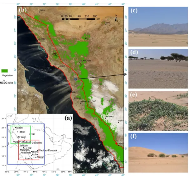
microphysi-Figure 1. (a)The CLM4 model domains (green and red), WRF-Chem domain (blue), and 16 ground observation stations.(b)Dust plume above the Red Sea observed by MODIS/TERRA at 07:45 UTC on 14 January 2009. Overview of the landscapes:(c)piedmont,(d)trees over the sand,(e)wild watermelons over the sand, and(f)sand dunes and scattered vegetation.

cal schemes (Marticorena and Bergametti, 1995; Shao, 2004; Shao et al., 2011b). Intermediate-complexity models use mi-crophysical parameterizations where possible but make sim-plifying assumptions and use empirical coefficients to short-cut complex calculations (Zender et al., 2003a). The total vertical mass flux of dustF (kg m−2_s−1_{), generated from the}

ground into the atmosphere, is calculated using the following equation:

F =T SfmQs 4

X

j=1

αjMj, (1)

whereT is a spatially uniform tuning constant that controls the average emission rate (see Sect. 2.4).

Thefmparameter is a grid cell fraction of soils suitable for

dust mobilization. It depends on the land fraction of bare soil (which is calculated dynamically depending on soil condi-tions), the plant functional type (PFT), leaf area index (LAI),

stem area index (SAI), and top soil layer water content, cal-culated within CLM4.

Theαj coefficients are sandblasting mass efficiencies for each of the four dust transport size binsj. They depend on the mass fraction of clay particles (CLY) in the soil, which is defined by SOILPOP30, a 30 s soil population dataset de-veloped by Nickovic et al. (2012) from STATSGO-FAO. This soil dataset is widely used in dust-related studies (e.g., Menut et al., 2013).

Mj is a mass fraction of dust size binj. The size bins approximate particles with diameters from 0.1 to 1 µm, from 1 to 2.5 µm, from 2.5 to 5.0 µm, and from 5 to 10 µm. In the original model formulation, the emission flux is calculated separately for each size bin. Here, we consider total emitted dust mass and therefore sum up fluxes from all the bins in Eq. (1).

Qs is the total horizontally saltating mass flux

(kg m−2_s−1_{). It is proportional to the third power of}

velocityu∗t:

Qs=

 



csρatmu3∗s

g

1− u∗t

u∗s

1+u∗t

u∗s

2

,foru∗s > u∗t

0 foru∗s≤u∗t,

(2) wherecs is the saltation constant equal to 2.61,ρatm is the

atmospheric density (kg m−3_{), andg is the acceleration of}

gravity (m s−2_{). Saltation wind friction velocityu∗} s is

cal-culated from wind friction velocity u∗ (m s−1_{) accounting}

for the Owen effect of increasingu∗ during saltation (Zen-der et al., 2003a). Threshold friction velocity u∗t is

calcu-lated within CLM4 as a function of surface roughness and soil moisture.

Sis a spatially varying dimensionless dust emission source function. It has a sense of soil erodibility and accounts for the susceptibility of soil to wind erosion (Webb and Strong, 2011). In the default CLM4 configuration S=1, assuming that the emission is calculated based on winds and avail-able surface and soil properties only. However, it has been reported recently that the models based on purely physical properties of soils represent quite inaccurate spatial patterns of dust emission, especially on the regional scale (Huneeus et al., 2011; Knippertz and Todd, 2012). This is caused by the deficiencies of parameterizations and inaccurate input infor-mation. Thus, the source functionSis introduced to improve the spatial distribution of dust emission simulations.

Different approaches have been discussed and a number of principles to calculate the source function recently intro-duced (Kim et al., 2013; Parajuli et al., 2014; Walker et al., 2009). Ginoux et al. (2001) proposed calculating the source function based on a topographic approach, assuming that the areas with topographic depressions are the most probable lo-cations for sediments to accumulate. The geomorphic source function (Zender et al., 2003b) is based on the assumption that dust emission is likely to occur from areas of poten-tial runoff collection. Similar to the topographic source func-tion, it only depends on elevation. Another family of source functions is instead based on observations (mostly remote sensing), assuming that the most active dust source areas are those where airborne dust is more frequently observed. The statistical source function introduced by Ginoux et al. (2010, 2012) uses Moderate Resolution Imaging Spectroradiometer (MODIS) estimates of aerosol optical depth and land cover data to identify the dust source areas.

In this study, we calculate source function using the dust aerosol optical depth (AODD) product developed by

Brind-ley and Russell (2009) and Banks and BrindBrind-ley (2013), based on high-frequency measurements from the Meteosat Sec-ond Generation Spinning Enhanced Visible and InfraRed Im-ager (SEVIRI) instrument. The SEVIRI instrument is lo-cated on board the Meteosat-9 geostationary satellite and provides measurements every 15 min (Brindley and Russell, 2009; Banks and Brindley, 2013), much more frequently than

MODIS. SEVIRI measurements were recently utilized to analyze dust sources in northern Africa (Schepanski et al., 2012; Evan et al., 2015). To calculate the source function we adopt the frequency method, first proposed by Prospero et al. (2002), and later used in a number of other studies (Gi-noux et al., 2010, 2012; Schepanski et al., 2012). It assumes that the intensity of a dust source is proportional to the fre-quency of occurrence of atmospheric dust:

S=N (AODD>AODt) / N (AOD), (3)

where statistical source functionS is defined in each loca-tion as a ratio of the number of events N(AODD> AODt)

when dust-caused AODDexceeds the threshold value AODt

to the total number of observationsN(AOD). The threshold is meant to filter out background dust and is usually cho-sen empirically (Schepanski et al., 2012). We have tested the thresholds in the range of 0.8–1.15 and found that the spatial patterns of the source functions are quite similar. The cho-sen threshold value of 1.12 is larger than the one used in the global study (Ginoux et al., 2012) but comparable to regional studies of Saharan dust sources (Schepanski et al., 2012). The choice of relatively large threshold was motivated by several reasons. First, the background dust AOD in Arabian Penin-sula is much higher than globally observed one. Second, SE-VIRI was shown to overestimate AOD under high humid-ity conditions and low dust loadings that are the case for the Red Sea coastal plain (Banks et al., 2013). Overall, this larger threshold allows us to better represent intensive dust sources, in contrast, for example, to Ginoux et al. (2010, 2012), who aimed at capturing and classifying smaller sources. Below we show that the source function based on high-frequency measurements significantly improves the simulation results. 2.3 Observations, metrics, and an overview of the

study area

The Red Sea environment has been identified as a zone of complex wind circulation (Langodan et al., 2014). Due to the strong land–sea diurnal temperature contrasts, land and sea breezes persist through the entire year. The large-scale circulation systems interact with breezes and are reinforced by orographic structures, which create a complex pattern of mesoscale circulation. The most prominent mesoscale fea-ture of the Red Sea is the Tokar Gap jet on the western coast (Davis et al., 2015, and references therein). Westward-blowing mesoscale jets also exist on the eastern coast (Gille and Llewellyn Smith, 2014; Jiang et al., 2009). These jets originate mostly in winter due to the cold/dry air outbreaks from the central Arabian Plateau and channel through a series of mountain gaps. They may last for several days and have a prominent diurnal cycle. The jets, along with the breezes, cause small-scale dust updrafts in the coastal area. The gen-erated dust plumes are sometimes observed by satellites over the Red Sea. For example, a dust storm with narrow dust plumes caused by the jet winds captured by MODIS/TERRA at 07:45 UTC on 14 January 2009 is shown in Fig. 1b.

In order to cover the study area, we run the CLM4 model over the two rectangular domains shown in Fig. 1a. Also shown are the meteorological observation stations that are used in the current study. We use hourly data from the In-tegrated Surface Dataset (ISD) developed by the National Climatic Data Center (NCDC) (Smith et al., 2011). We se-lected 15 stations in Saudi Arabia and 1 station in Jor-dan inside the CLM4 domains with continuous observation records for 2009–2011. The stations provide meteorological observations including weather code and visibility reports. The automated visibility measurement and manned weather code observation are reported on an hourly basis, but the weather code is only present when visibility reduces to below 10 000 m. Otherwise, just a constant visibility of 10 000 m is reported (indicating fair weather). The weather codes that correspond to the presence of dust are 06 (dust in suspen-sion), 07 (dust raised), 08 (dust whirl), and 09 and 30 to 35 (dust storm). Most of the weather stations (except that in Makkah) are located on the site of regional or interna-tional airports, thus the data archive was primarily assembled from SYNOP or METAR/SPECI weather reports (Smith et al., 2011).

Although the station visibility measurements are only in-directly related to the amount of locally emitted dust, they are one of the most relevant data sources for assessing dust emission fluxes in the absence of other observations. These data are frequently used in dust-related studies. For example, the present weather code reports from meteorological records have been used for evaluation of dust event frequency and dust climatology (Cowie et al., 2014; Goudie and Middle-ton, 2006; Hamidi et al., 2014; Notaro et al., 2013; Shao and Dong, 2006; Wang et al., 2011; Yu et al., 2013). In some other studies, these observations were used to derive soil erodibility fields (Shao, 2008). The parameterization formula for assessing near-surface dust concentration based on

visi-bility measurement has also been proposed (Camino et al., 2015, and references therein; Rezazadeh et al., 2013; Shao et al., 2003). Mahowald et al. (2007) used the station vis-ibility measurements to study dust sources and stated that visibility-derived observations should better capture the tem-poral variability in surface dust fluxes compared to AOD measurements. But still, these data cannot serve as a quanti-tative measure of model performance, being non-automated (in the case of weather code) and being highly influenced by remote dust transport, the presence of water vapor, and dust physical properties and composition (Shao, 2008). Another limitation of station observations is a weak sensitivity to low and moderate reductions in visibility that is only reported and complemented by the weather code when it drops be-low 10 000 m. Camino et al. (2015) also note that clear skies are often reported under hazy atmospheric conditions when dust is present. Thus, we do not expect our analysis to give an absolute assessment of model emissions but rather to allow comparison of different model configurations.

We apply several metrics to compare the model statistics of dust events with station data, making use of both weather code reports and visibility measurements. First, we assess the temporal variability in dust event frequency and intensity, correlating the monthly-averaged time series. We follow the classical definition of dust event frequencyFd from hourly

weather code reports (Shao and Dong, 2006):

Fd=Nd/Ntot, (4)

whereNdis the number of reported dust events andNtot

is the total number of reports (including those when visibil-ity was not reduced below 10 000 m and no weather code was reported). All of the weather codes indicating the presence of dust (i.e., 06 to 09 and 30 to 35) were considered correspond-ing to a dust event. Based on this definition, we construct the monthly-averaged time series, so that the frequency is calcu-lated separately for each month. To obtain the model estimate of dust event frequency, we calculate it as a fraction of time when hourly-averaged emission is above the certain thresh-old. We apply two constant thresholds of 1 and 4 µg m−2_s−1_,

approximately corresponding to 70th and 85th quantiles of hourly emission rates. Taking the fraction of the time with dust emission above the threshold during the month, we ob-tain the model monthly time series of dust event frequency.

An approach alternative to sampling was proposed in Ma-howald et al. (2007). The authors noted the scarceness of weather code reports and proposed to filter non-aerosol (fog-driven) visibility reductions based on dew-point temperature measurements. In our case, we prefer a sampling approach as most of the station visibility reduction measurements are complemented with weather codes.

Both of the metrics described above reflect the primarily temporal, not spatial, variability in the model results. We ap-ply the metrics to different model configurations and, as their basic effect is aimed at improving the spatial patterns, no sig-nificant differences are found. Thus, some other metrics are needed to assess the reliability of dust emission spatial distri-butions. The technique we propose for assessing spatial pat-terns of dust emission is to sample the hourly visibility time series by dust event reports, choosing the time steps when a dust event was reported, and to calculate the daily, and then 3-year mean visibility for each station. The mean emission rate is also calculated from model data sampled for the same time steps. Station data are sampled to correspond to hourly instantaneous model output; thus, SPECI reports that usually take place between regular reports are not considered. We therefore obtain two samples of 3-year-averaged station dust intensity and model emission rate (with the sample length equal to the number of stations) and calculate the correlation coefficient between them.

We calculate correlation coefficients between samples that reflect diverse highly nonlinear physical phenomena. As we do not have the physical ground to assume the linear rela-tion between these phenomena, we use Spearman’s rank cor-relations instead of Pearson’s corcor-relations for all cases. The dust emissions and station visibility are negatively correlated, whereas the opposite is true of station dust frequency. For the sake of simplicity, here we report the emission–intensity cor-relations with reversed sign, keeping both coefficients posi-tive.

2.4 MERRAero and dust emission calibration

Very recently, a few aerosol reanalysis products have become available (Buchard et al., 2016; Inness et al., 2013). In this study, we utilize the dust emissions from MERRAero devel-oped by NASA (Buchard et al., 2016), which was calculated using meteorological fields from the Modern-Era Retrospec-tive Analysis for Research and Applications (MERRA I) (Rienecker et al., 2011). The reanalysis has a spatial reso-lution of 50×50 km and is available from 2003 onwards. MERRAero is built on the Goddard Earth Observing System version 5 (GEOS-5) atmospheric model, which comprises an aerosol module based on a version of the Goddard Chem-istry, Aerosol, Radiation, and Transport (GOCART) model (Chin et al., 2002; Ginoux et al., 2001). GOCART simulates the interactive cycle of dust, sulfate, sea salt, black, and or-ganic carbon aerosols. MERRAero assimilates AOD obser-vations from the MODIS sensor flying both on TERRA and

on AQUA satellites. The GOCART dust scheme in GEOS5 uses a topographic source function (Ginoux et al., 2001).

It is a common approach for atmospheric dust calculations to use calibration based on observations of total AOD (or assimilate AODs as in the MERRAero), as it is the basic observed quantity that characterizes an amount of aerosols in the atmosphere (Kalenderski et al., 2013; Prakash et al., 2015; Zhao et al., 2010, 2013). However, in our offline CLM4 simulations we do not calculate AOD and therefore cannot compare our results with the observed AOD directly (Shi et al., 2016). In the absence of quantitative measurements of dust generation the direct model validation is not possible (Laurent et al., 2008; Bergametti and Forêt, 2014). Therefore, we calibrate the model emissions integrated over the entire coastal area using the dust emissions from MERRAero. We note that it is difficult to expect a global reanalysis with a relatively low spatial resolution to produce detailed spatially resolved estimates of dust emission over a narrow coastal zone. The coastal plain is only covered by one or two grid boxes (in width) by the MERRAero grid. On the other hand, the reanalysis captures the enhanced dust activity area on the western coast of the Arabian Peninsula and its integral (over the entire coastal area) multi-year estimates of dust emission from approximately 150 000 km2area is a reasonable refer-ence point for model calibration. Although MERRAero dust emission has not been validated directly, the recent paper of Ridley et al., (2016) reported better seasonality of dust AOD in MERRAero compared to other datasets and pointed to po-tentially better dust emission patterns due to finer spatial res-olution and representation of surface winds. Thus, we rely on the MERRAero estimate of 2009–2011 annual dust emis-sion from the coastal plain (7.5 Mt) and set theT constant in Eq. (1) to produce the same dust amount in CLM4. The scaling factor depends on whether the dust emission source function is used or not. The values of scaling factors ap-plied in our experiments are given in Table 4. We also exam-ined the Monitoring Atmospheric Composition and Climate (MACC) reanalysis product available from ECMWF (Cuevas et al., 2015; Bellouin et al., 2013), but its spatial resolution of 80×80 km is coarser than that of MERRAero and it does not capture the enhanced dust emission from the coastal plain.

2.5 WRF-Chem simulations

from Kalenderski et al. (2013), who performed a 1 km run for the period of 1–20 January 2009, which included sev-eral major dust outbreaks from the Arabian Peninsula across the Red Sea. Additionally, we have performed a finer-scale 4 km simulation for 1–31 January 2009, but in a smaller spa-tial domain focused on the Red Sea coastal plain (Fig. 1). The experiment setup is generally identical to Kalenderski et al. (2013). The main difference is that we use a more sophis-ticated eight-bin Model for Simulating Aerosol Interactions and Chemistry (MOSAIC) (Zaveri et al., 2008) and photo-chemical Carbon Bond Mechanism (CBM-Z) (Zaveri and Peters, 1999). Another update is that instead of topographic source function (Ginoux et al., 2001) used in Kalenderski et al. (2013), to be consistent with the current study, we use the SEVIRI source function described in Sect. 2.2. Kalenderski et al. (2013) calibrated the dust emission calculations based on AOD observation from Solar Village AERONET station (see the previous section). As there are no AERONET sta-tions in the smaller domain of our WRF-Chem simulation, we calibrate our model run using AODs from Kalenderski et al. (2013) (Fig. S1 in the Supplement).

3 Sensitivity analysis

The dust emission parameterizations calculate dust influx in the atmosphere using meteorological fields, land-surface physical properties, and, sometimes, empirical proxy infor-mation about land-surface erodibility (see Eq. 1). Here we use the improved datasets of soil and vegetation physical properties and high-frequency source function as input for our dust generation calculations. To evaluate the effect of these improved input datasets on dust generation, we use the same meteorological fields fixed in all sensitivity simu-lations. Firstly, we assess the sensitivity of the parameterized dust emissions to varying spatial resolution of land-surface characteristics. Secondly, we apply the dust emission source function and test the results using weather station data.

3.1 Sensitivity to the horizontal resolution of surface data

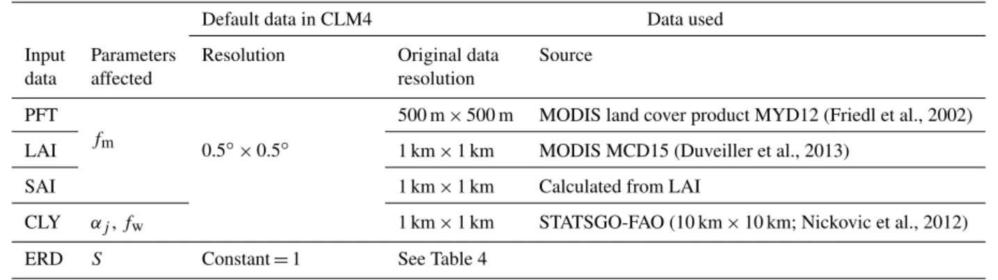
Shi et al. (2016) discussed CLM4 sensitivity to the type and resolution of vegetation datasets for the entire Arabian Penin-sula. They quantified the impact of high-resolution surface characteristics derived from MODIS measurements com-pared to the default ones on dust emission in the Arabian Peninsula. They found that dust emission is most sensitive to surface vegetation, especially in sparsely vegetated areas, which is the case for the western coastal plain. Here, we ex-tend the sensitivity study of Shi et al. (2016) to finer scales, examining the sensitivity to the horizontal resolution of PFT, LAI, SAI, and CLY (clay mass fraction) fields. The descrip-tion of those datasets is given in Table 2.

First, we consider the sensitivity of dust emissions, when changing the spatial resolution of each of the input surface characteristics separately. We perform a control experiment with all of the surface data taken at 10 km×10 km reso-lution (10kmALL), and four additional simulations. In the 10kmLPFT, 10kmLLAI, and 10kmLCLY experiments, we degrade the spatial resolution of one of the datasets (PFT, LAI, or CLY, respectively) in comparison with 10 kmALL to 50 km×50 km. In the 50kmALL experiment, the spatial resolution of all of the above characteristics is degraded to 50 km×50 km. Wind forcing and model grid resolution of (10 km×10 km) are kept the same for all simulations. See the definition of all relevant experiments in Table 3. Spatially uniform tuning constantT =0.011 is used in all experiments (Table 4) based on 10kmALL calibration. It is important to mention thatT does not affect the spatial patterns of emis-sion, which is the primary focus of our attention in these ex-periments.

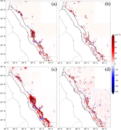
The differences between annual mean dust generation in 10kmALL and other simulations are depicted in Fig. 2a–c. Overall, using high-resolution vegetation results in an ap-preciable increase in total dust generation with comparable contribution from PFT and LAI datasets. The changes are not strictly additive, as the emission process is nonlinear, and are spatially non-uniform. Total dust emission from the coastal plain in 50kmALL is around 10 % smaller than in 10kmALL. The partial differences are smaller: 6 % (10kmL-LAI) and 3 % (10kmLPFT). The spatial structure of dust gen-eration changes with the increased resolution of vegetation datasets is spatially non-uniform. The highest differences occur along the mountain areas with substantial vegetation cover (Fig. 1a). Locally, in the central and southern parts of the coastal plain, dust generation may increase by more than 50 % (Fig. 1c). In some areas south of the coastal plain, high-resolution PFT leads to decreasing of dust emissions. The difference between the 10kmALL and 10kmLCLY sim-ulation is not shown, as the changes are very small (less than 1 g m−2_a−1_{). The likely explanation for the low model}

sensi-tivity to soil texture dataset resolution is that its data sources may initially have been based on relatively coarse-resolution observations, which have subsequently been reinterpolated to a finer grid.

Table 2.Land surface data used in model setup.

Default data in CLM4 Data used

Input Parameters Resolution Original data Source

data affected resolution

PFT

fm _0.5◦_×0.5◦

500 m×500 m MODIS land cover product MYD12 (Friedl et al., 2002)

LAI 1 km×1 km MODIS MCD15 (Duveiller et al., 2013)

SAI 1 km×1 km Calculated from LAI

CLY αj,fw 1 km×1 km STATSGO-FAO (10 km×10 km; Nickovic et al., 2012)

ERD S Constant=1 See Table 4

Table 3.Spatial resolution of input datasets used in simulations.

Simulation

10kmALL 50kmALL 1kmALL 10kmLPFT 10kmLLAI 10kmLCLY

Input data

PFT 10 km 50 km 1 km 50 km 10 km 10 km

LAI & SAI 10 km 50 km 1 km 10 km 50 km 10 km

CLY 10 km 50 km 1 km 10 km 10 km 50 km

Wind forcing 10 km

3.2 Model test with station data

In this section, we compare the model results with observa-tions at meteorological staobserva-tions, keeping in mind the limita-tions of this approach discussed in Sect. 2.3. To obtain the model values at station locations, we use bilinear interpo-lation from four surrounding grid points. If bilinear inter-polation is not possible (for the coastal stations), the near-est neighbor grid point is used. First, we assess the model’s ability to capture the temporal variability in dust generation in the region on monthly scales. The temporal variability in model dust emissions is mostly driven by the wind forcing. As the wind forcing is the same for all experiments, it is not surprising to find that correlation coefficients are similar in all model simulations. Therefore, we show the results for both dust event frequency (Fig. 3a) and intensity (Fig. 3b) based on 10kmALL simulation only.

For most of the stations, there are positive correlation co-efficients of dust event frequency, ranging from 0.3 to 0.7 with the mean value of 0.47±0.15 for 1 µg m−2_s−1

thresh-old and 0.52±0.14 for 4 µg m−2_s−1_{threshold. Most of the}

correlations are statistically significant at the 95 % level, sug-gesting reasonable model skill. For Jeddah, Bisha, and Mad-inah, correlations become significant when a larger threshold is applied, and for Najran and Abha, only correlations with the smaller threshold are significant. The intensity correla-tions are not fully independent from frequency, as average visibility drop is related to the number of dust reports (in the case of severe dust storms, there are usually a number of

con-current reports that increase the frequency estimate). Despite that, we report visibility-based correlations of intensity, as these measurements are used for the spatial metrics. The re-sults are slightly worse than for dust frequency with the mean correlation around 0.4±0.2 for both thresholds, but correla-tions are still significant for 12 stacorrela-tions out of 16. Overall, the obtained correlations demonstrate a good model ability to simulate the monthly variations of dust activities.

Figure 2.Differences between annual mean dust emission in model simulations (g m−2a−1):(a)10kmALL–10kmLLAI,(b)10kmALL– 10kmLPFT,(c)10kmALL–50kmALL, and(d)1kmALL–10kmALL.

Figure 3.Spearman’s correlation coefficients for monthly-mean series of(a)dust event frequency and(b)intensity between station data and results from 10kmALL experiment.(c)Spatial metrics of model performance (see text for definition) for three basic experiments with and without SEVIRI source function.

measurements from AERONET were also proposed in Ma-howald et al. (2007).

The results obtained in the current study are consistent with those proposed by Mahowald et al. (2007) and Yu et

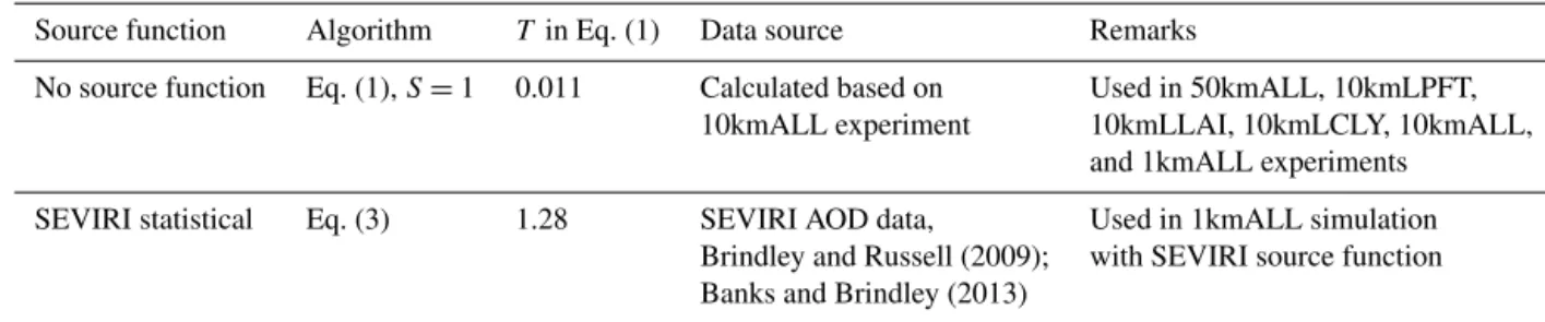
Table 4.Tuning constants used in the simulations.

Source function Algorithm T in Eq. (1) Data source Remarks

No source function Eq. (1),S=1 0.011 Calculated based on Used in 50kmALL, 10kmLPFT, 10kmALL experiment 10kmLLAI, 10kmLCLY, 10kmALL,

and 1kmALL experiments

SEVIRI statistical Eq. (3) 1.28 SEVIRI AOD data, Used in 1kmALL simulation Brindley and Russell (2009); with SEVIRI source function Banks and Brindley (2013)

could be explained by local dust generation. On the other hand, Yu et al. (2013) also suggested that dust is not a pre-dominant aerosol over the Red Sea coastal plain. This state-ment was questioned recently by Osipov et al. (2015), who reported, based on the CALIPSO lidar measurements during 2007–2013, that the ratio of the “not dust” to “dust” success-ful retrievals over this area is 2.04 %.

To assess the spatial distribution of simulated dust emis-sions and choose the best model settings, we use the metrics described in Sect. 2.3. The model and station data are sam-pled to include the visibility reductions during dust reports only. The number of reported dust events per station during the 3 years considered in the study ranges from less than 100 at two stations (72 dust reports in Makkah and 64 dust re-ports in Al Wajh) to up to 400. Given this, the two stations with the lowest numbers of observations are excluded from the final spatial analysis. The Al Wajh station is situated just several hundred meters away from the seashore, and the low number of dust reports may be due to small-scale circula-tion features. Model and satellite dataset resolucircula-tion may be not enough to represent the local circulation, surface char-acteristics and emission rate with the desired accuracy. As for the Makkah station, the low number of dust reports may be caused by instrumentation errors and insufficient quality control; the station is not collocated with the airport and the data are not used in aviation services.

The spatial correlations with station samples are calcu-lated for three basic simulations (50kmALL, 10kmALL, and 1kmALL) with and without the statistical source function (Fig. 3c). The results show that using the SEVIRI source function significantly improves the spatial structure of dust emission. Even our short-sample statistics allow high corre-lations to be obtained for all of the three basic simucorre-lations. Increasing the surface datasets’ resolution, together with ap-plying the source function, leads to increasing the correla-tion coefficient to 0.68, 0.77, and 0.85 depending on the ba-sic simulation. The correlation coefficients for simulations without source functions are not statistically significant. The 50kmALL correlation is almost zero, whereas correlations in 10kmALL and 1kmALL experiments are almost equal. This result is expected, implying high-resolution datasets only add small-scale details that are difficult to capture with a coarse observational network.

Along with the SEVIRI source function, we use several others (see Sect. 2.2). However, topographic, geomorphic and MODIS-based source functions are all unable to signifi-cantly increase the model skill. For topographic and geomor-phic source functions this can be explained by the fact that they were developed for large-scale models initially; thus, they are not expected to work well on regional scales. The MODIS source function, on the other hand, is based on mea-surements from a polar-orbiting satellite that has low tempo-ral resolution (only two measurements per day), insufficient to capture the local dust phenomena caused primarily by cir-culations with a prominent diurnal cycle (Ginoux and Torres, 2003; Kocha et al., 2013; Yu et al., 2013) (see Sect. 4.3).

4 Dust emission multi-year estimate

The above analysis shows that 50kmALL, 10kmALL, and 1kmALL model configurations with the source function based on high-frequency satellite measurements provide quite realistic results (spatial correlation with respect to ob-servations of 0.68, 0.77, and 0.85). The 1kmALL simulation with the SEVIRI source function has the highest resolution and correlation coefficient; therefore, we use it for further analysis of dust emission climatology and discuss the major dust source areas within the coastal plain, diurnal, and sea-sonal cycles of emission from those areas, as well as their annual mean and variability.

4.1 Emissions from the main dust sources

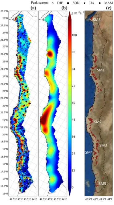
We first address the spatial distribution of dust-generating ar-eas (hot spots), and then turn to the temporal variability. To examine the dust generation regime, we discuss the 3-year-averaged (2009–2011) spatial patterns of total generated dust amount (Fig. 4), dust emission frequency, intensity, and max-imum emission rate (Fig. 5). Dust emission hot spots are defined as areas where generated dust amount and emission frequency are 2 times higher, and dust event intensity is 1.5 times higher than domain-averaged values. The locations of hot spots are shown by shaded areas on a real-color satellite image (Fig. 4c).

Figure 4.Annual dust emission (g m−2a−1) in(a)1kmALL exper-iment with SEVIRI source function (2009–2011);(b)MERRAero (2003–2015).(c)Main dust emission hot spot areas mapped on real-color satellite image. Peak season is indicated by symbols (see fig-ure legend).

special attention to dust generation mechanisms in the hot spot areas. Although the period of 3 years is quite short to be considered climatologically representative, it is shown below that dust generation in this area generally has low interannual variability. In the current and subsequent sections, we use the same threshold for frequency and intensity (4 µg m−2_s−1_{) as}

for calculation of correlation coefficients with observations. The total dust emission is spatially variable, chang-ing from zero to more than 100 g m−2_a−1 _{in some areas}

(Fig. 4a). Figures 4a and 5a–b depict a similar pattern, sug-gesting that the areas with the largest and most frequent dust outbreaks coincide. The dust emission hot spots occupy

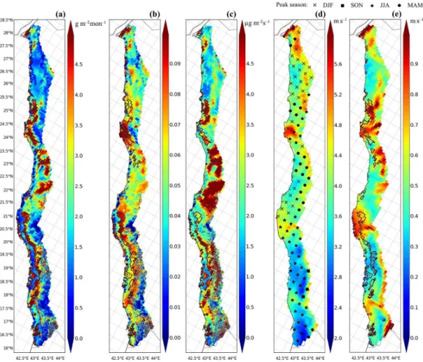
Figure 5.Average 2009–2011(a)dust event frequency,(b)average emission intensity (µg m−2_s−1_{), and (c)yearly maximum} emis-sion rate (µg m−2s−1) in 1kmALL experiment with SEVIRI source function. Peak season is indicated by symbols (see figure legend).

around 8 % of the total coastal area (Fig. 4c). The zones where the maximum emission rate occurs (Fig. 5c) agree well with the hot spots. Most of the hot spots correspond to lowlands. The hot spots are located not directly near the coastal areas, but rather near the western hillsides of the He-jaz Mountains, in the dry riverbeds (“wadis”) where allu-vial deposits are available. The primary hot spot zone in the northern part of the study area (SM1, Fig. 5c) spans along the coast between the cities of Yenbo and Umluj. Emission inten-sity reaches its maximum value here (over 12 µg m−2_s−1_),

and emission frequency is over 0.25. As seen from Fig. 6d, this hot spot is mostly driven by high winds. Dust event fre-quency is highly variable here, which is explained by the wind forcing variability (Fig. 6e). Dust generation and wind forcing peak in spring. These hot spot conditions are preva-lent in this part of the coastal plain.

Figure 6.Standard deviations of monthly(a)total dust emission (g m−2_month−1_{),(b)dust event frequency, and(c)average emission} intensity (µg m−2s−1) in 1kmALL experiment with SEVIRI source function. Average 2009–2011 WRF forcing(d)wind speed (m s−1), and(e)its monthly standard deviation (m s−1_{). Peak season is indicated by symbols (see figure legend).}

the proximity of Al Bahah (SM3). A third small but inten-sive zone is located on a coast near the city of Al Qunfudhah (SM4). The frequency of dust events is around 0.25 in these southern hot spot areas, and emission intensity reaches more than 10 µg m−2_s−1_.

The SM2 hot spot is driven by moderate winds with con-siderable intermonth variability; thus, the frequency of dust activity changes during the year, having its peak in summer months. In the rest of the southern hot spots (SM3 and SM4, Fig. 5c), wind activity is weak (Fig. 6d) and dust emission is mainly facilitated by the low erosion threshold and is in-creased due to source function correction. The intermonth variability in dust emission is relatively low here and is pre-dominantly driven by dust frequency variations. There are two other smaller, isolated emission zones: a hot spot near the Gulf of Aqaba in the north (SM6, Fig. 5c) and an inten-sive hot spot area in the south near Jizan (SM5, Fig. 5c).

Dust emission in the large area between 21 and 24◦_N is relatively uniform and reaches quite a considerable vol-ume. Although there are no major hot spots, this area con-tributes significantly to the total dust generation, producing

around 2 Mt of dust per year. The annual-mean dust fre-quency is around 0.15 here, and the average dust intensity is 7–9 µg m−2_s−1_{, with both of them reaching maximum in}

winter. Dust generation shows high intermonth variability, but in contrast to SM1, the variability is mostly caused by variations in dust emission intensity. Examining the wind circulation in this area, we find that the high variability in dust event intensity is caused by high monthly mean val-ues in winter and early spring. Dust intensity averaged over this part of the coastal plain reaches 36 µg m−2_s−1 _during

a January 2009 dust storm and 28 µg m−2_s−1_{during March}

character of dust generation, these wind gusts may lead to high monthly values of dust generation intensity. Similar pro-cesses also occur in the north of the SM1 hot spot.

To further confirm this idea we analyze the WRF-Chem simulations discussed in Sect. 2.5. The jets that originate in the coastal plain and bring dust over the Red Sea are both ob-served by satellites and simulated in the models (Fig. S1 in the Supplement). The spatial patterns of dust generations in WRF-Chem and CLM4 simulations are consistent (Fig. S2 in the Supplement). However, the magnitude of dust emis-sion in the models varies. In the 20-day simulation by Kalen-derski et al. (2013), 1.39 Mt of dust is generated compared to 0.66 Mt in CLM4. In the WRF-Chem–MOSAIC run per-formed in the current study, 1.5 Mt of dust is produced dur-ing January 2009 compared to 0.92 Mt in CLM4. Thus, the daily average dust generation from the coastal plain in WRF-Chem is 40–50 % larger than in CLM4 which is in the range of expected uncertainty between offline and coupled dust simulations.

The annual mean spatial distribution of dust emission in MERRAero for the period of 2003–2015 is depicted in Fig. 4b. Due to its coarse resolution, MERRAero hardly re-solves the local-scale emission areas. Nevertheless, the dust generation pattern reasonably agrees with the results ob-tained with the high-resolution model and features the pri-mary emission zones. Two major emission zones in Fig. 4b can be identified as SM1 and SM2, although SM1 is smaller than in our results and its peak generation is further to the north. The SM2 source area is the strongest, covering large neighboring territories. MERRAero generates some dust in the area of SM3 and SM4 hot spots, although the amount is less than in CLM4. The emission zone near Jizan (SM5) is also present in the reanalysis. Overall, the dust emission pat-terns from CLM4 and independent reanalysis are quite con-sistent. Below we show that CLM4 dust emission seasonal cycles are consistent with reanalysis as well.

4.2 Temporal variability in dust emissions 4.2.1 Seasonal cycle of dust emissions

The seasonal and interannual variability in dust storms in the Arabian Peninsula has been extensively discussed in re-cent studies (Alobaidi et al., 2016; Notaro et al., 2013, 2015; Rezazadeh et al., 2013; Shalaby et al., 2015; Yu et al., 2013, 2015). Most of the studies report that the period of maxi-mum dust activity is from February until July–August, but the peak month varies depending on location and data source (Notaro et al., 2013; Shalaby et al., 2015; Yu et al., 2013). In the north of the Arabian Peninsula, late winter – early spring peak is more common, and in the south-southeast desert re-gions dust activity tends to reach its maximum in summer. According to Notaro et al. (2013, and references therein), the late winter–early spring dust peak in the northwest is due to the cold fronts associated with cyclones from the

Mediter-ranean, whereas the summer peak in the south is due to di-urnal heating, turbulent mixing, and strong summer Shamal winds (Yu et al., 2015). In this study, we find the seasonal-ity of dust emission from local sources to be quite consistent with previously reported results.

The seasonal cycles (averaged over 3 years) of total dust generation, monthly mean dust frequency, intensity, and monthly maximum emission rate are shown in Fig. 7. The analysis is conducted over the entire coastal domain and separately for the northern and southern parts (separated at 21◦_{N) of the coastal plain and hot spot areas. To compare} our model results with reanalysis, the corresponding values from MERRAero averaged over 2003–2015 are also plotted together with standard deviation intervals.

The total emission flux (Fig. 7a) exhibits a pronounced seasonal cycle with a dual maximum in March and July and minimum in February and October. The peaks originate from a distinct character of seasonal cycles in the northern and southern parts of the coastal plain. The March peak is only evident in the northern area and is mostly caused by increased intensity during the dust storm episodes (Fig. 7c). High intensity is also seen in January in the north, partially caused by a dust storm in 2009. The peak winter and spring seasons for dust intensity in the north are also shown in Fig. 5b. Conversely, the July peak is due to both frequency (Figs. 5a and 7b) and intensity (Figs. 5b and 7c) reaching their maximums in the southern part of the coastal plain, al-though they are lower than that in the northern coastal plain. The seasonal cycle of maximum dust emission rate (Fig. 7d) generally follows that of intensity. Overall, we can conclude that the different climate and surface conditions in the north and south of 21◦_{N drive the spatial variations of the seasonal} cycle of dust emission.

The seasonal cycle of dust emissions from the hot spots is consistent with the seasonal variability in the total dust generation from the coastal plain. Since the hot spots are in both the northern and southern parts of the coastal plain, the seasonal cycles of total emissions are smoother than for the northern and southern coastal plain separately. In the hot spots, magnitudes of dust frequency, intensity, and maximum emission rate are 2–2.5 times higher than that for the total coastal area and are above the mean plus standard deviation threshold in MERRAero. The overall amount of dust emit-ted from the hot spot areas is 1.9 Mt a−1_{, or 25 % of the total}

emissions, while hot spots occupy only 12 800 km2 or less than 10 % of the total area. This fact indicates that the soil mineralogical composition and wind variability have to first be studied in these hot spot areas (Prakash et al., 2016).

re-Figure 7.Average seasonal cycles of monthly(a)total dust emission (Mt month−1),(b)dust event frequency,(c)average emission inten-sity (µg m−2s−1), and(d)maximum emission rate (µg m−2s−1) in 1kmALL experiment with SEVIRI source function (2009–2011) and MERRAero (2003–2015). MERRAero standard deviation intervals are shown by shading.

analysis. One of the possible reasons is the coarse resolution of reanalysis that does not capture the local-scale wind pat-terns that cause the spring peak. Similarly, Yu et al. (2013) re-ported that satellite AOD measurements in the western Ara-bian Peninsula do not feature the early spring peak (as op-posed to station dust records), attributing it to the local char-acter of springtime dust generation.

With the exception of the March peak, the seasonal cy-cle of CLM4 dust generation lies within the MERRAero standard deviation interval. This is also true for dust event frequency and intensity, although the frequency is slightly smaller than in reanalysis and intensity is slightly larger. It may be caused by the fact that, in the case of MERRAero, these quantities were calculated with the same threshold, but based on 3-hourly data; therefore, some dust outbreaks on the threshold borderline are missed. As expected, maximum dust emission rates in CLM4 are larger than in reanalysis, being substantially above the standard deviation interval, especially in March and July.

The total annual dust emission from the entire 147 000 km2 coastal area is 7.5 Mt, as in MERRAero. This dust influx in the atmosphere is substantial and, assuming that a significant portion of this dust could be transported to the Red Sea, may cause dust deposition to the Red Sea comparable to that of 6 Mt a−1_{from the major dust}

storms (Prakash et al., 2015). About 4.9 Mt a−1_{, or 65 % of}

the total emission, is generated from the northern part of the coastal plain. Analyzing dust emission in MERRAero for the entire 2003–2015 period, we find it varies only slightly

7.5±0.5 Mt a−1_{. Small interannual variability in emissions}

and a permanent distribution of the dust hot spots (Figs. 6a–c and 7) suggest that the coastal plain is a stable dust source. 4.2.2 Diurnal cycle of dust emissions

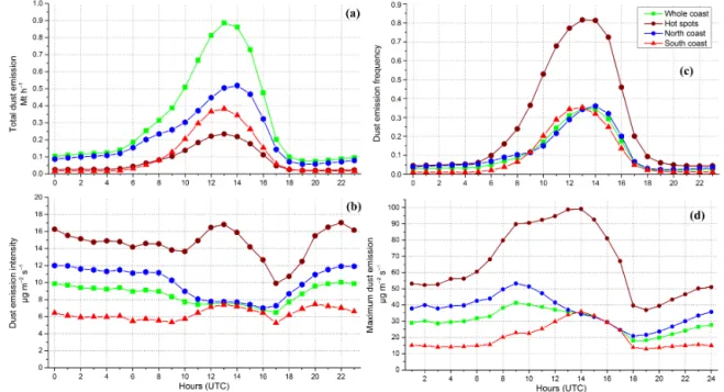
The annual average diurnal cycles of total dust generation, frequency, intensity, and maximum emission rate are com-puted from the 3-year simulations (Fig. 8a–d). Total dust gen-eration, frequency, and maximum emission rate have a pro-nounced diurnal cycle, consistent with wind speed intensify-ing durintensify-ing solar peak. Both total dust emission and frequency peak around the early afternoon, at 12:00–14:00 UTC, with a slight shift between the northern and southern parts of the coastal plain due to the latitudinal extent. The frequency of dust events during the daily maximum is around 0.35 both in the north and in the south. Overall, around 80 % of air-borne dust is generated between 07:00 and 16.00 UTC. The nighttime dust emission in the northern part is much stronger due to the larger number of cold fronts passing through the northern Red Sea (Notaro et al., 2013; Yu et al., 2015). In the south, the frequency of nighttime dust events is lower due to the different character of wind forcing with a more pro-nounced diurnal cycle (Notaro et al., 2013). The frequency of dust events in the hot spot areas during the peak hours reaches 0.8, but during the nighttime it is less than 0.05.

Figure 8. Annual mean diurnal cycles of (a) total dust emission (Mt h−1), (b) dust event frequency, (c) average emission intensity (µg m−2s−1), and(d)maximum emission rate (µg m−2s−1) in 1kmALL experiment with SEVIRI source function (2009–2011).

a large number of moderate-intensity events; thus, the aver-age emission is relatively small. On the other hand, the small total number of dust events above the threshold in the night-time leads to a larger contribution from strong events and in-creased average intensity. The diurnal range of emissions in the northern coastal plain is from 7 to 12 µg m−2_s−1_{. In the}

southern part, the nighttime intensity is smaller due to the presence of areas with zero contribution to the average inten-sity, as there are no dust events exceeding the threshold in-tensity. This results in an almost uniform diurnal intensity cy-cle in the southern part of the coastal plain (5–7 µg m−2_s−1_).

In the hot spot areas, average dust intensity has two diurnal peaks at 13:00 and 22:00 UTC and reaches the minimum at 17:00 UTC.

The diurnal cycle of dust maximum emission rate is also different in the north and south. It peaks at 09:00 UTC in the northern areas with a diurnal range of 20–50 µg m−2_s−1_,

and at 14:00 UTC in the south with a diurnal range of 15– 35 µg m−2_s−1_{. The maximum emission rate averaged over}

the coastal plain follows the one in the north, but the peak value is smaller (40 µg m−2_s−1_{). In the hot spot areas, the}

diurnal cycle of maximum emission rate is even more pro-nounced. Daily maximum emission peaks during 09:00– 15:00 UTC and reaches 100 µg m−2_s−1_{. It is still}

signifi-cant during the nighttime, reaching more than 50 µg m−2_s−1_.

High nighttime values of dust emission intensity and maxi-mum emission rate in the hot spot areas despite low event frequency indicate that the rare, severe nighttime dust gener-ation is much more pronounced in the hot spots compared to other areas of the coastal plain.

4.3 Mineralogical composition

Dust elemental composition has a variety of physical and biogeochemical impacts. Perlwitz et al. (2015), Scanza et al. (2015), and Zhang et al. (2015) have applied sophisti-cated modeling tools to study the dust mineral composition on global scales. In our case, we concentrate on a fine-scale narrow coastal area, as generated dust has the potential to deposit directly to the sea. Thus, we aim at estimating the amount of minerals generated from the coastal plain and as-sume it is representative of the mineral composition of dust deposited to the Red Sea. To calculate the emitted mineral fluxes we use the global datasets of dust mineral composi-tion, GMINER30, and soil texture, SOILPOP30, developed by Nickovic et al. (2012). SOILPOP30 provides the global coverage of fractions for three soil texture classes (clay, silt, and sand). GMINER30 provides the soil type and corre-sponding mineral composition. We assume that the relative proportions of minerals in the airborne dust are the same as those of the parent soils. The largest size bin of emitted dust (transport bin) in CLM4 is 5–10 µm, whereas the silt fraction in GMINER30 corresponds to 2–50 µm. This allows us to as-sume following Nickovic et al. (2013) that emitted dust is a mixture of clay and silt particles only (without coarser frac-tions). Thus, emitted mineral fractions are weighted with the clay and silt content in the soil. For minerals that are present in both clay and silt, the weighted values are summed.

Figure 9.Annual mineral emission fluxes (Mt a−1) in 1kmALL ex-periment with SEVIRI source function (2009–2011).

it does not always hold in the general case (Claquin et al., 1999; Perlwitz et al., 2015). During the airborne dust life cycle, both chemical (dust aging) and physical fractionation processes occur and change the dust mineral composition and size distribution. However, due to the short pathway from the coastal plain to the sea, dust composition changes due to gravitational settling and chemical transformations become less important for local dust particles compared to those sub-jected to long-range transport. Another issue is the instru-mental bias of GMINER30 dataset that was produced using the wet sieving technique. This technique strongly disperses soil aggregates (Shao, 2001; Laurent et al., 2008; Perlwitz et al., 2015), adding uncertainty to the partitioning of miner-als between clay and silt fractions. However, Nickovic et al. (2012) assume the same fraction of phosphorus and nearly the same of iron oxides in clay and silt. These minerals are our primary interest, as they limit the marine productivity, and thus the instrumental bias is less important. Nickovic et al. (2012) assume the same fraction of phosphorus and nearly the same of iron oxides in clay and silt. Having said this, we note that our assessment may serve as an initial rough esti-mate of the mineral composition of dust deposited in the sea from local sources.

The minerals’ annual emissions are calculated using dust emission flux obtained with the 1kmALL simulation and the SEVIRI source function applied. Figure 9 shows annual amounts of minerals emitted from the coastal plain. Quartz is the most abundant mineral, comprising around 40 % of the total emission. A total of 25 % of the total emission corre-sponds to feldspars, followed by illite, smectite, kaolinite, calcite, gypsum, hematite and goethite (the iron source), and phosphorus. The Arabian Red Sea coast provides 76±5 kt of

iron oxides and 6±0.4 kt of phosphorus annually. Over 60 % of iron oxides and phosphorus are emitted from the northern part of the coastal plain, acting as a nutrition source for the oligotrophic northern part of the Red Sea. Although only a portion of dust emitted from the Arabian coast is deposited to the Red Sea, due to the close proximity of the dust gener-ation area to the sea (especially in the northern coastal plain) and the structure of mesoscale circulation that includes jets and breezes, its role in total mineral deposition to the Red Sea could be significant.

5 Conclusions

This study focused on the dust emission from the Red Sea Arabian coastal plain. We applied the offline CLM4 land-surface model to perform high-resolution simulations of dust emission for 2009–2011 using up-to-date land-surface datasets. The magnitude of integrated over the entire area dust emissions was tuned to fit the estimate from MER-RAero, while the spatial structure was calculated within CLM4, forced by 10 km×10 km resolution meteorology from WRF simulations. To test the simulated dust emission, we developed the corresponding metrics and performed a comparison with the weather station reports of horizontal visibility and present weather code. We obtained significant correlations for monthly time series of dust event frequency and intensity (station-mean correlation coefficients of 0.5 and 0.4), indicating reasonable model performance. The results confirmed that dust emission from local sources on the Ara-bian Red Sea coastal plain is significant and supported the hypothesis by Yu et al. (2013) that the dust activity in this area may be caused by local-scale dust outbreaks.

Within the proposed framework, we performed a sensitiv-ity study and demonstrated that high-resolution input surface datasets may add fine-scale details to dust generation pat-terns. The spatial resolution of vegetation datasets was shown to alter total dust emissions by up to 10 %. We confirmed the findings by Shi et al. (2016), showing that the increased res-olution of the vegetation dataset leads to significant dust flux in some zones where it was very weak when coarse input data fields were used. We estimated the comparable contri-bution to total dust emission from the increased resolution of the plant functional type dataset on the one hand and the leaf area index and stem area index on the other.

Following the evaluation tests, we based our estimates on model simulation with 1 km×1 km spatial resolution and SEVIRI source function. The estimate of total dust emission from the coastal plain, tuned to fit emissions in the MER-RAero, is 7.5±0.5 Mt a−1 _{(approximately 50 g m}−2_a−1_).

Over 65 % of dust is generated in the northern part of the coastal plain. The seasonality of dust emission differs sub-stantially in the northern and southern parts of the coastal plain. In the south, the annual maximum of dust emission occurs in July, whereas in the north March is the peak month of dust activity. This distinct character is due to the contrast-ing forccontrast-ing mechanisms: in the north, emission is caused by strong, diurnally variable, cold season winds, whereas in the south it is largely controlled by a low erodibility threshold and soil moisture. These features result in dual maximum values within the seasonal cycle of total dust emission from the coastal area in March and July.

The spatial pattern of total annual dust emission is highly non-uniform, reaching more than 100 g m−2a−1in some hot spot areas. The chain of hot spots stretches alongside the coastal zone, with most of them located in the lowlands near the western hillsides of the Hejaz Mountains – riverbeds that are usually considered the source of alluvial material. The hot spots occupy around 8 % of the coastal area and gener-ate over 25 % (1.9 Mt a−1_{) of total dust. The emission pattern}

is in reasonable agreement with the coarse-resolution results from the MERRAero global reanalysis, despite the fact that the reanalysis dust model uses a different source function. We also showed that dust generation has a pronounced diurnal cycle. Around 80 % of dust is generated during the daytime, between 07:00 and 16.00 UTC, with dust emission rate and emission frequency peaks during the early afternoon (12:00– 14:00 UTC).

The total dust generation from the coastal plain of 7.5±0.5 Mt a−1_{is comparable to the estimate of annual dust}

deposition to the Red Sea of 6 Mt a−1 _{due to major dust}

storms (Prakash et al., 2015). Small interannual variability indicates that the study area is a stable dust source. The com-parison with the short-term WRF-Chem simulations suggests that this estimate could be even larger, as WRF-Chem pro-duces 40–50 % more dust, supporting the finding that the coastal plain is a significant dust source. Our calculations of the dust mineralogy suggest that 76±5 kt of iron oxides and 6±0.4 kt of phosphorus are emitted from the coastal plain annually.

6 Data availability

All the data and model results used in this study are available from the authors upon request.

The Supplement related to this article is available online at doi:10.5194/acp-17-993-2017-supplement.

Author contributions. Anatolii Anisimov performed the data pro-cessing, developed the technique for comparison with observations, conducted the comparison with reanalysis, performed the WRF-Chem simulation, formulated the results, and wrote the final paper. Weichun Tao designed the experiments, ran the model simulations, calculated the source functions, performed the basic analysis, and wrote the paper draft. Georgiy Stenchikov formulated the problem, directed the research, and edited the paper. Stoitchko Kalenderski ran the WRF model to obtain the meteorological forcing for the dust emission calculations. P. Jish Prakash and Weichun Tao worked to-gether on the dust mineral analysis. Zong-Liang Yang, one of the developers of CLM4, helped in setting the CLM4 runs. Mingjie Shi and Weichun Tao worked together on collecting the land-surface data.

Acknowledgement. We thank V. Ramaswamy and Paul A. Ginoux of GFDL for valuable discussions. We also thank Johann Engel-brecht and Linda Everett for proofreading the article. The research reported in this publication was supported by the King Abdullah University of Science and Technology (KAUST). For computer time, this research used the resources of the Supercomputing Laboratory at KAUST in Thuwal, Saudi Arabia.

Edited by: K. Tsigaridis

Reviewed by: three anonymous referees

References

Acker, J., Leptoukh, G., Shen, S., Zhu, T., and Kempler, S.: Remotely-sensed chlorophyll a observations of the northern Red Sea indicate seasonal variability and influence of coastal reefs, J. Mar. Syst., 69, 191–204, doi:10.1016/j.jmarsys.2005.12.006, 2008.

Ackerman, S. A. and Cox, S. K.: Surface weather observations of atmospheric dust over the southwest summer monsoon region, Meteorol. Atmos. Phys., 41, 19–34, doi:10.1007/BF01032587, 1989.

Alobaidi, M., Almazroui, M., Mashat, A., and Jones, P. D.: Arabian Peninsula wet season dust storm distribution: region-alization and trends analysis (1983–2013), Int. J. Climatol., doi:10.1002/joc.4782, 2016.

Baker, A. R. and Croot, P. L.: Atmospheric and marine controls on aerosol iron solubility in seawater, Mar. Chem., 120, 4–13, doi:10.1016/j.marchem.2008.09.003, 2010.

Banks, J. R. and Brindley, H. E.: Evaluation of MSG-SEVIRI mineral dust retrieval products over North Africa and the Middle East, Remote Sens. Environ., 128, 58–73, doi:10.1016/j.rse.2012.07.017, 2013.

Banks, J. R., Brindley, H. E., Flamant, C., Garay, M. J., Hsu, N. C., Kalashnikova, O. V., Klüser, L., and Sayer, A. M.: Intercom-parison of satellite dust retrieval products over the west African Sahara during the Fennec campaign in June 2011, Remote Sens. Environ., 136, 99–116, doi:10.1016/j.rse.2013.05.003, 2013. Barkan, J., Kutiel, H., and Alpert, P.: Climatology of dust