www.atmos-chem-phys.net/10/3119/2010/ © Author(s) 2010. This work is distributed under the Creative Commons Attribution 3.0 License.
Chemistry
and Physics
What can we learn from European continuous atmospheric CO
2
measurements to quantify regional fluxes – Part 2: Sensitivity of flux
accuracy to inverse setup
C. Carouge1, P. J. Rayner1, P. Peylin1,2, P. Bousquet1,3, F. Chevallier1, and P. Ciais1
1Laboratoire des Sciences du Climat et de l’Environnement, UMR1572, CNRS-CEA-UVSQ, Bˆat. 701,
Orme des Merisiers, 91191 Gif-sur-Yvette, France
2Laboratoire de Biog´eochimie et Ecologie des Milieux Continentaux, CNRS-UPMC-INRA, Paris, France 3Universit´e de Versailles Saint-Quentin en Yvelines, Versailles, France
Received: 7 August 2008 – Published in Atmos. Chem. Phys. Discuss.: 28 October 2008 Revised: 22 December 2009 – Accepted: 8 March 2010 – Published: 31 March 2010
Abstract. An inverse model using atmospheric CO2
obser-vations from a European network of stations to reconstruct daily CO2fluxes and their uncertainties over Europe at 50 km
resolution has been developed within a Bayesian framework. We use the pseudo-data approach in which we try to recover known fluxes using a range of perturbations to the input. In this study, the focus is put on the sensitivity of flux accu-racy to the inverse setup, varying the prior flux errors, the pseudo-data errors and the network of stations. We show that, under a range of assumptions about prior error and data error we can recover fluxes reliably at the scale of 1000 km and 10 days. At smaller scales the performance is highly sensitive to details of the inverse set-up. The use of tempo-ral correlations in the flux domain appears to be of the same importance as the spatial correlations. We also note that the use of simple, isotropic correlations on the prior flux errors is more reliable than the use of apparently physically-based er-rors. Finally, increasing the European atmospheric network density improves the area with significant error reduction in the flux retrieval.
Correspondence to:C. Carouge (claire.carouge@lsce.ipsl.fr)
1 Introduction
Quantitative understanding of the sources and sinks of chem-ically and radiatively important trace gases and aerosols is essential in order to assess the human impact on the envi-ronment. Observations of atmospheric concentration provide the basic data for inferring sources and sinks at the surface of the Earth, or in the volume of the atmosphere. For conser-vative tracers, which stay inert once emitted, the influences of surface fluxes are modified only by atmospheric trans-port, which integrates the flux heterogeneity over regional and continental scales. Starting from a set of atmospheric concentration observations, and using a model of the atmo-spheric transport and chemistry, it is possible to infer infor-mation about the distribution of sources and sinks at the sur-face. This process is known as inversion of the atmospheric transport.
In the companion paper (Carouge et al., 2010, CA08) we investigated the ability of an atmospheric network to con-strain sources and sinks of CO2over Europe. In particular,
work in a real case but we can be confident that if an inver-sion setup is unsuccessful with pseudo-data it is unlikely to work in realistic conditions.
There are many decisions in setting up an inversion. The choice of a particular spatial resolution to execute an inver-sion is tightly related to the degree of confidence we attribute to our biogeochemical knowledge on spatial heterogeneity of the fluxes and their errors. If one strongly trusts the correct-ness of the prior spatial structure of the sources and sinks as usually defined by models of ecosystems, or of air-sea fluxes, one needs to use only a few number of regions to solve for, whereas if not, one must increase the resolution of the solu-tion.
Here we tackle the problem of inverting daily Net Ecosys-tem Exchange (NEE) from daily atmospheric concentrations over Western Europe, using pseudo-data. In this context, there is little biogeochemical knowledge about the space and time coherence of modeled NEE and its errors within a con-tinent. Only one comparison between the results of a vegeta-tion model and the observed daily NEE at a few tens of eddy-covariance sites was realized so far (Chevallier et al., 2006). This study suggests that the NEE errors possess strong tem-poral correlation (up to several weeks) but no obvious spatial correlation. In this context, a logical inversion setup would be to consider as many regions as possible (i.e. every grid point of the model) but with correlated prior uncertainties, with correlations informed by the knowledge of flux errors. Very little is known on the structure of flux errors at the scale used in this study, we thus realized different scenario.
In this paper, we perform three categories of sensitivity tests to investigate the influence on the inversion results of 1) the parametrisation of the prior flux errors structure, 2) the errors attached to the atmospheric pseudo-observations, and 3) the density of the atmospheric station network. The latter is studied by comparing the 10 stations network of the control case with a denser network of 23 stations, reflecting the evolution of European network. As in CA08 we invert pseudo-data, generated with a forward run of the transport model prescribed with an arbitrary “true” NEE flux from an ecosystem model. The prior, or first guess, NEE is given by another, independent, ecosystem model. Our main criteria for assessing the inversion accuracy are the error reduction, and the ability to retrieve the true fluxes when starting from the erroneous prior. We first describe the control inversion (S0, CA08) setup and the sensitivity tests (Sect. 2), then we analyze the inversion accuracy (Sect. 3) for each of the sen-sitivity tests. Conclusions are drawn in Sect. 4.
2 Grid-based regional inversion and sensitivity tests
2.1 Control inversion (S0)
2.1.1 Overall setup
The Bayesian synthesis inversion formalism is used (Enting, 2002). We invert CO2fluxes each day over a European grid,
which has the same spatial resolution as the transport model (50 km). The input information is a time-series of simulated, daily CO2 concentration from a network of European
sta-tions. The pseudo-data framework allows us to test the im-pact of different inversion setups on the accuracy of the so-lution. This will be done by comparing the retrieved fluxes with the “true fluxes” used to generate the pseudo-data. The goal is to optimize daily land-ecosystem CO2fluxes (NEE)
over Europe, and daily air-sea fluxes over the Northeastern Atlantic. It is assumed that, outside these two regions, all the fluxes are perfectly known and are not optimized. We construct separately the true and the a priori NEE fluxes us-ing two independent terrestrial ecosystem models (see be-low). The time series of pseudo-data are generated for year 2001 by the LMDZ transport model, prescribed with true fluxes from the ORCHIDEE ecosystem model (Krinner et al., 2005). These pseudo-data are further perturbed with Gaus-sian noise, in order to account for data errors and, in an ide-alized way, for model representation errors. Technically, we divide the inversion during one year into a series of consec-utive 3-monthly inversions, (see CA08 for details). The per-formance of the inversion will be analyzed by comparing: 1) the optimized fluxes with the true fluxes (error diagnostic), and 2) the optimized flux uncertainties with the a priori un-certainties (error reduction diagnostic).
2.1.2 Calculation of the sensitivity of concentrations to
surface fluxes
We use the LMDZ global transport model with 19 sigma-pressure layers (Sadourny and Laval, 1984, Hourdin and Ar-mengaud, 1999). The grid of the model is zoomed over Western Europe, with a maximum resolution of 50 km by 50 km. The modeled winds are nudged to the analyzed fields of the European Center for Medium Range Weather Fore-casting (ECMWF) for the year 2001. The sensitivity of daily CO2 concentration at a given station and time step to all
the surface fluxes is called the influence function (also the Green’s function). The influence function of each datum is calculated with the LMDZ retro-transport (Hourdin and Tala-grand, 2006), where a pulse of “retro-tracer” is emitted each day and transported backwards in time. In this formulation, the sign of the advection term is reversed, and the sign of the unresolved diffusion terms is unchanged. Computing the sensitivity of one daily CO2observation to all the fluxes is
2.1.3 Construction of pseudo-data
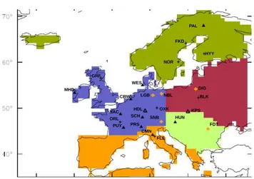
We rely on a European network of 10 stations, as it existed in 2001 in the CARBOEUROPE cluster of projects (see Fig. 1). The pseudo-data are generated with LMDZ for that year, pre-scribed with “true” daily NEE from the ORCHIDEE model. For inverting the fluxes, the modeled CO2pseudo-data are
selected for daytime only, between 11:00 and 16:00 local time, and their influence functions calculated accordingly. This daytime selection strategy is currently applied by mod-elers simulating continuous CO2data (Geels et al., 2007;
Pe-ters et al., 2007; Law et al., 2008), and by experimentalists taking flask samples. This selection recognizes the difficul-ties of large-scale models simulating nocturnal CO2trapping
near the ground during the growing season. In the control inversion S0, only a small noise with a standard deviation 0.3 ppm, representative of instrumental noise, is added to the pseudo-data (CA08).
2.1.4 A priori fluxes and errors
These errors are as in CA08. The CO2fluxes over all the
re-gions outside Europe and the Northeast Atlantic (see Fig. 1) are not optimized. For each grid-point of the Northeastern Atlantic region, the prior air-sea flux is set to zero, with a small total regional error of±0.05 GtC/year. The prior air-sea flux errors are spatially correlated between ocean grid-points, with an exponential decrease with distance (e-folding length of 1500 km). Some temporal correlations are consid-ered with an exponential decrease with time (e-folding time of 10 days) but no cross-correlations are applied. For each grid point of Europe, the prior daily NEE is taken from the TURC model (Lafont et al., 2002). TURC is a diagnostic NEE model driven by climate data and satellite observations of NDVI for the period April 1998–April 1999. The dif-ferences between fluxes produced by biospheric models are principally driven by differences in the meteorological con-straints and the differences in the internal structure of the models. The fact that TURC has a very different structure from ORCHIDEE, used to produce the true fluxes, and that it is integrated with climate forcing of a different year, maxi-mizes the difference between prior and true NEE. From these differences, we assess an average prior daily flux standard deviation error of 3 gC m−2day−1for each grid-point. The structure of terrestrial flux correlations varies between sensi-tivity tests and is presented in the next section for each test.
2.2 Sensitivity tests
2.2.1 Prior flux errors (SP tests)
In addition to S0, we ran four sensitivity tests with a distinct a priori NEE error covariance. A summary of the error char-acteristics and of the total European NEE prior error for each test is given in Table 1:
SAC OXK
NBL LGB
HDL SCH
PRS
CMN FLE
HUN
FDT KPS
BLK DIG
PUY ORL
CBW WES
MHD GRF
HYY
NOR FKD
PAL
SNB
Fig. 1. Map of European continuous stations. The 2001 AERO-CARB stations are represented by black filled triangles, CarboEu-rope stations by black empty triangles, CHIOTTO tower by black crosses and WDCGG stations by orange stars. After inversion, fluxes were aggregated over five different regions: “Western Eu-rope” in blue, “Mediterranean EuEu-rope” in orange, “Balkans” in light green, “Central Europe” in red and “Scandinavia” in green.
S0. Control inversion setup, with both spatial and tempo-ral correlation being defined by an exponential attenuation, with an e-folding time of 10 days and an e-folding distance of 1000/1500 km over land/ocean. This setup, detailed in CA08 is also called “isotropic flux correlation”. Note that the e-folding time length was chosen from the autocorre-lation in time of the NEE differences between TURC and ORCHIDEE that shows for each grid-point an exponential decrease, withR≈0.3 after 10 days. We choose to neglect cross-correlations in time and space. Then each of the spa-tial and temporal covariance matrices need to be divided by 2 before to add them together (CA08). In this way, we ensure the mathematical properties of the total covariance matrix.
SP1. Test with no spatial and no temporal correlations be-tween grid points, also called “No-correlation”.
SP2. Test with temporal but no spatial correlations, called “time-only correlation”. There are no cross-correlations, so the factor 0.5 is not applied and the resulting temporal corre-lations are higher than the correcorre-lations used in S0 case.
SP3. Test with spatial but no temporal correlations, called “distance-only correlation”. Here again, there are naturally no cross-correlations, so the spatial correlations are higher than the correlations used in S0 case.
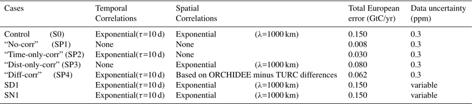
Table 1.Name of the different inversions and flux error correlations used in each case.
Cases Temporal Spatial Total European Data uncertainty
Correlations Correlations error (GtC/yr) (ppm)
Control (S0) Exponential(τ=10 d) Exponential (λ=1000 km) 0.150 0.3
“No-corr” (SP1) None None 0.008 0.3
“Time-only-corr” (SP2) Exponential(τ=10 d) None 0.030 0.3
“Dist-only-corr” (SP3) None Exponential (λ=1000 km) 0.080 0.3
“Diff-corr” (SP4) Exponential(τ=10 d) Based on ORCHIDEE minus TURC differences 0.062 0.3
SD1 Exponential(τ=10 d) Exponential (λ=1000 km) 0.150 variable
SN1 Exponential(τ=10 d) Exponential (λ=1000 km) 0.150 variable
Table 2. List of European continuous stations with their location and additional stations for SN1.
Station Station Latitude Longitude Altitude
name symbol (m a.s.l.)
Cabauw CBW 51.97◦N 4.92◦E 200
Monte Cimone CMN 44.18◦N 10.70◦E 2165
Hegyhatsal HUN 46.95◦N 16.65◦E 363
Mace Head MHD 53.32◦N 9.88◦W 25
Pallas PAL 67.97◦N 24.12◦E 560
Plateau Rosa PRS 45.93◦N 7.70◦E 3480
Puy de Dˆome PUY 45.75◦N 3.00◦E 1465
Saclay SAC 48.75◦N 2.17◦E 120
Schauinsland SCH 47.92◦N 7.92◦E 1205
Westerland WES 54.93◦N 8.32◦E 8
Diabla Gora DIG 54.15◦N 22.07◦E 157
Fundata FDT 45.47◦N 25.30◦E 1383
Neuglobsow NBL 53.17◦N 13.03◦E 65
Sonnblick SNB 47.05◦N 12.98◦E 3106
Waldhof LGB 52.80◦N 10.77◦E 74
Heidelberg HDL 49.40◦N 8.70◦E 116
Kasprowy KPS 49.22◦N 19.99◦E 1987
Bialystok BLK 52.25◦N 22.75◦E 300
Florence FLE 43.82◦N 11.26◦E 245
Griffin GRF 56.55◦N 2.99◦W 232
Orl´eans ORL 46.97◦N 2.12◦E 203
Norunda NOR 60.08◦N 17.47◦E 102
Hyyti¨al¨a HYY 61.84◦N 24.28◦E 73
Flakaliden FKD 64.12◦N 19.45◦E 57
Ochsenkopf OXK 50.03◦N 11.80◦E 1185
error structure is more complex than in the S0 case (Fig. 2). The cross-correlations are also discarded in this case, in the same way than in S0 case.
For all experiments, prior fluxes over land are assigned standard deviations of 3 gC m−2day−1. Because we ne-glect cross-correlations in case S0 and SP4, correlations are smaller (factor 2) compared to the initial “space-only” and “time-only” correlation matrices (SP2 and SP3). Note that
-1 -0.6 -0.2 0.2 0.6 1
b) a)
Fig. 2.Example of correlations for a point in Germany (symbolised
with a black triangle) for correlations in distance(a)and
correla-tions based on TURC and ORCHIDEE fluxes difference for 1 Jan-uary 2001(b).
2.2.2 Data errors (SD test)
We consider in addition to S0, a sensitivity test with larger random errors on the daily pseudo-data, which intend to rep-resent the random part of transport model errors. In all cases, the daily data errors are not correlated spatially and tempo-rally in the data error covariance matrix. Note also that flux error reduction does not depend on the value of the concen-tration data, but only on its prior uncertainties (Sect. 3.2).
S0. Control inversion setup. A small white noise of stan-dard deviation 0.3 ppm is assumed (CA08). This small noise is representative of instrumental noise.
SD1. Test with a larger noise added to the pseudo-data. We add to the pseudo-data a noise with a realistic value based on temporal variability of real observations, and corresponding to the typical error that could be used in an inversion with real observations. Following Peylin et al., 2005, daily er-rors are calculated as the standard deviation of actual hourly (or half-hourly) CO2measurements, each day between 11:00
and 16:00. The underlying assumption to link this error cal-culation to the random part of error in transport modeling is that atmospheric transport models tend to be less reliable for sites and days with larger hourly variability (Geels et al., 2007). The resulting annual mean daily error varies between 0.56 ppm at Pallas, up to 2.84 ppm at Cabauw. In summer, the seasonal mean daily error varies between 0.84 ppm at Plateau Rosa, up to 3.51 ppm at Schauinsland. In winter, the data error ranges between 0.29 ppm at Pallas up to 2.63 ppm at Cabauw. In winter, plain stations, like Cabauw, are more likely to present large variability in their measurements. In-deed, the planetary boundary layer (PBL) is low in winter. Thus, plain stations are likely to measure blobs of concen-trated air from time to time. At the opposite, mountain sites measure almost exclusively the free troposphere in winter. Thus the measurements at these sites are likely to show lit-tle variability. At the opposite in summer, the PBL is more developed. The plain sites measure then a more uniformly mixed air than in winter. At the opposite, the mountain sites are more likely to measure air from free troposphere and the PBL. The variability in their hourly measurements is then enhanced compared to winter. In the SD1 setup, the flux er-ror reduction reflects more realistically the erer-ror reduction structure of actual data. Yet, this data error setup might not account completely for the lack of ability (and the system-atic biases) of a transport model with a resolution of 50 km to reproduce faithfully a point-scale measurement.
2.2.3 Network of stations (SN test)
All previously described inversion tests have been conducted with 10 European continuous stations, as operational in 2001 (Fig. 1). However, the European atmospheric CO2network
is still growing, both in spatial (more stations) and temporal (more continuous stations) density.
SN1. Test with 13 new stations added to the 2001 Euro-pean network. To do so, the influence functions are cal-culated for additional pseudo-stations with LMDZ. We re-strict the SN sensitivity test to three months in summer in order to avoid a too large computation time. We use the er-ror reduction as a measure of the “power” of a denser net-work. The calculation of this term only requires the influ-ence function and the data error for each new observation. For data errors, we adopted the case of a large noise, as de-scribed in the SD1 test above and thus compared the SN1 inversion to the SD1 inversion. Three groups of new stations are added to the network in the SN1 test. The first group contains five stations which are measuring CO2
continu-ously and reporting data to the World Data Center for Green-house Gases (WDCGG, http://gaw.kishou.go.jp/wdcgg/), but which are not inter-calibrated with the high-precision CAR-BOEUROPE network (Fig. 1). Their data errors are taken as the daily standard deviations of available hourly observa-tions, as for other sites. The second group contains two con-tinuous sites, Heidelberg and Kasprowy, which became part of the CARBOEUROPE-IP project after 2001 (see Fig. 1; http://ce-atmosphere.lsce.ipsl.fr/). The errors at both sites are set to the average error of the 2001 network, excluding Hegy-hatsal and Cabauw stations. The third group contains six tall towers, which progressively became operational as part of the CHIOTTO project (http://www.chiotto.org/). These tall towers (Fig. 1) were assigned a summer mean error identical to the one of the Hegyhatsall tower in Hungary (2.24 ppm).
3 Results
We analyze in this section the sensitivity of the accuracy of the inversion to the different setups described in Sect. 2. To focus on synoptic changes, we only compare deseasonalized fluxes (see CA08). The results from the control inversion S0 of CA08, briefly summarized below, are then systematically compared with those of each sensitivity test.
3.1 Control inversion results
Correlation NSD
C/ SP2
E/ SP4
Time aggregation (days)
1.8 > 2 1 1.2 1.4 1.6 0.2 0.4 0.6 0.8
0 B/ SP1 A/ Control
S
p
a
c
e
a
g
g
re
g
a
tio
n
(
k
m
)
D/ SP3
0.8 0.95
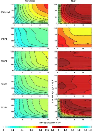
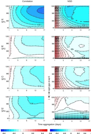
Fig. 3.Evolution of correlation and NSD with spatial and temporal aggregation for the posterior flux residuals of the control(a), SP1
(b), SP2(c), SP3(d)and SP4(e)inversions.
the densest network, the NEE can be reasonably well recon-structed, withR >0.63 and NSD≈1. The maximum values ofRreached 0.75 at the scale of the entire western European region, for a 15-days aggregation scale. For other European regions, the true fluxes could not be accurately reconstructed, due to the sparse atmospheric observing network (CA08).
3.2 Sensitivity to prior flux error correlations (SP tests)
Figure 3b–e display for the four SP sensitivity tests theR
and NSD statistics between inverted and true fluxes (desea-sonalized) as a function of space (y-axis) and time (x-axis) aggregation. We also discuss the statistical significance of the correlations and variance differences as in CA08, using confidence interval for a Gaussian law and F-variance tests, respectively (Saporta, 1990). At the 95% level, we obtain, for 365 daily values, a confidence interval of±0.1 for the correlations.
In all cases, we found NSD>1 (Fig. 3), which reflects the fact that the inversion cannot entirely correct for the much larger variability of the prior NEE in TURC as compared to ORCHIDEE. This result confirms the dependence of the re-sults on the prior in Bayesian inversions but also suggests the overall procedure may work better with an improved prior.
SP1. With no correlations of prior NEE errors, the inver-sion accuracy is degraded, as shown by comparing SP1 to the control inversion S0 results (Fig. 3b vs. Figs. 3a, 6a). A maximum value ofR=0.4 is reached, while NSD always lies above 1.15. The evolution ofR and NSD as a function of space and time aggregation is similar for SP1 as for S0 (Fig. 3 of CA08), showing that aggregation does not improve the in-version accuracy, except for NSD corresponding to spatial aggregation>1000 km. The statistical significance analysis shows no statistical differences between SP1 and the prior for correlations and variances (not shown). These limited improvements in the estimated fluxes from the prior fluxes illustrate the fact that prior flux error covariances are critical to spread the information content of concentration measure-ments to a large domain (Kaminski et al., 1999).
SP2. As mentioned in Sect. 2.2, including only temporal error correlations in the inversion does not directly compare to S0 because of the construction of the prior flux error ma-trix. We thus mainly compare SP2 to SP1 and SP3 cases. SP2 case clearly improvesRand NSD statistics compared to SP1 case but with still intermediate results between S0 and SP1. We obtainR=0.6 when aggregating the optimized fluxes each 15 days over the large western European region and the re-sponse ofR to aggregation (Fig. 3c) is similar to that of S0 but weaker. Almost independent of the temporal aggregation scale, the NSD steeply drops toward 1.1, i.e. the inversion ac-curacy is dramatically improved, when increasing the spatial aggregation scale from 40 to 200 km. For spatial aggregation higher than 200 km, only marginal NSD changes are found (Fig. 3c). This indicates that in SP2, the spatial aggrega-tion is the limiting factor controlling the inversion accuracy at scales smaller than 200 km (see also discussion in CA08). SP3. Including only spatial error correlations in the prior NEE, we obtain R values that are slightly degraded com-pared to the case with temporal prior error correlations only (SP2). A maximum value ofR=0.55 is reached for the west-ern European region, given a temporal aggregation of 15 days (Fig. 3d). This result is very similar to SP2. The response of NSD to aggregation is also similar to SP2, except for small spatial scales (<200 km) where NSD remains close to 1. In this case, the spatial prior error correlation plays an important role in correcting for large prior NEE variability compared to the truth, which was not the case in SP2.
a comparable role in spreading the atmospheric information to neighboring grid-points in the inversion.
SP4. In this more complex sensitivity test, the flux error correlations are patterned according to the NEE differences between truth and prior (see Sect. 2.2). The value ofR is smaller than in the control inversion S0, reaching up to 0.5 only (Figs. 3e and 6d). Correlations are statistically different between S0 and SP4 only for time aggregations longer than 9 days and spatial aggregations larger than 1000 km. The NSD as function of aggregation has about the same shape as in S0, with a slight improvement at large spatial (>1000 km) and small temporal (<7 days) scales compared to S0 but a deterioration at small spatial scale (<300 km). The sig-nificance analysis indicates no statistical difference for the residual variances between S0 and SP4 with both cases not being statistically different to the variances of ORCHIDEE true residual fluxes for time aggregation longer than 3 days at all spatial aggregations. At small spatial scales (<300 km) the inversion accuracy in SP4 is worse than in S0, with NSD isolines parallel to the temporal axis (Fig. 3e). Overall, at small spatial/small temporal scales, the NSD improves sim-ilarly in space and in time in SP4 and S0, indicating a bal-anced contribution of temporal and spatial error correlations to improve the flux variability retrieval.
It is rather surprising that the SP4 sensitivity test, with “physically-based” error correlations based on differences between TURC and ORCHIDEE, degrades on average the inversion accuracy as compared to the “isotropic” error cor-relations of S0, both in terms ofRand NSD. The reasons for this are linked to the computation of the error correlations in SP4 (using the variation of true minus prior fluxes over 5 days) and also because 1) prior and true fluxes are gener-ated using two very different models, and 2) these models calculate daily NEE forced by two different years of meteo-rology. Regarding point 2, different synoptic weather events affecting NEE in TURC and ORCHIDEE induce day-to-day changes in error correlation between grid-points, which have a poor coherence during a 5-day window. The resulting NEE error correlations thus strongly vary with time, and may show some sudden swings between large positive and large nega-tive values, even across grid-points that are far apart from each other. In this case, inconsistencies between prior mi-nus true NEE and prior error covariances might occur when considering all European grid-points. On the contrary, a smoother and isotropic prior flux error structure, such as pre-scribed in S0 always produces correlations that are constant in time and rapidly decrease with increasing distance across grid points (R is only 0.3 at 1000 km). For this case, in-consistencies between prior minus true NEE and prior error covariances are likely to be more restricted in space. It is also important to keep in mind that eachRor NSD value in Fig. 3 represents the mean of an ensemble of values correspond-ing to all possible spatial/temporal groups of grid points at a given aggregation scale during one year. We found, when calculatingR and NSD in the SP4 sensitivity test, that for
Correlation NSD
S
p
a
c
e
a
g
g
re
g
a
tio
Time aggregation (days)
1.8 >2
1 1.2 1.4 1.6
0.2 0.4 0.6 0.8
0 0.95 0.8
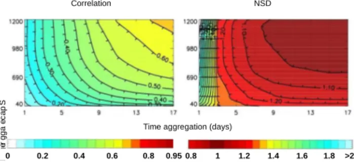
Fig. 4.Same as Fig. 3 for posterior fluxes of “dist correl” inversion of “transport error” case.
each level of space/time aggregation, the spread between the individual R and NSD values is larger than in the control inversion S0. This indicates that the SP4 error correlation patterns happen to be more favorable for some groups of grid points during specific periods. On average, the prior er-ror correlation matrix defined with the SP4 sensitivity test is more selective in terms of possible directions for the NEE er-ror corrections, as compared to the isotropic S0 case, which does not favor any particular spatial direction at any time. It turns out that the simpler isotropic choice is more neutral, and appears to be more robust for obtaining an accurate re-trieval of the daily fluxes in our framework. Finally, we also checked that, using a longer time window to build the spatial flux error correlations (10 days), the SP4 prior error correla-tion matrix becomes closer to the matrix of S0, so that theR
statistics are then more comparable between the two setups. In addition, we note that the NSD close to 1 for all ag-gregations in SP2 and SP3 contrasts with the large NSD ob-served in S0 and SP4 cases for small temporal and space ag-gregations. This suggests that larger prior flux error correla-tions (spatially or temporally) effectively constrain flux vari-ations at high resolution. The implementation of a full prior flux error correlation matrix, including cross-correlation be-tween space and time, in the inversion might thus be a poten-tial way to improve the results at small aggregation scales. It could be interesting to study a correlation matrix with cross-correlations in future work to estimate the validity of this as-sumption.
3.3 Sensitivity to data errors (SD test)
For the SD1 sensitivity test, where the data errors are larger and more realistic than in the control inversion, Fig. 4 shows the dependency ofRand NSD as a function of space and time aggregation. The results of SD1 are close to those obtained when assuming a smaller data error in S0, with only a small degradation of the inversion accuracy. On a daily basis, the
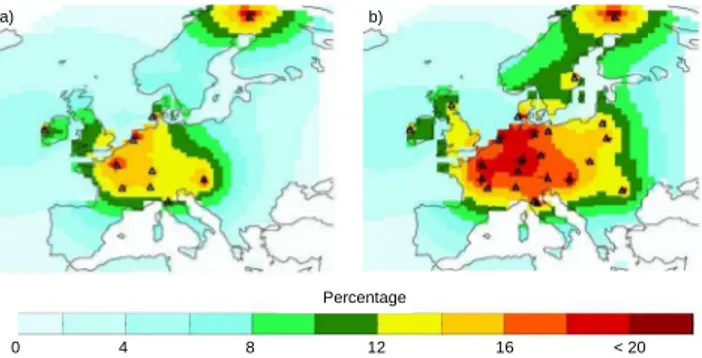
0 4 8 12 16 < 20 Percentage
a) b)
Fig. 5. (a)Three monthly average of daily error reduction for June-July-August for the “dist correl” inversion of “transport error” case.
(b)Same as (a) for an extended network.
shorter than 7 days). However, at the scale of the Western European region, and for a 10-day aggregation, bothR and NSD come very close to the results obtained in S0. This find-ing is encouragfind-ing for usfind-ing inversions to determine regional fluxes, because if a larger data error worsens the retrieval of daily fluxes, it has no strong consequences in the retrieval of weekly spatially-aggregated fluxes. However, the results of the SD1 test should not be generalized to the full impact of transport model uncertainties on inversion results. We only considered random data errors here, whereas a large part of the model-data mismatches arise from unresolved local pro-cesses/topography (representation error) or from wrong mix-ing parameterizations. Such errors may not disappear with averaging.
3.4 Sensitivity to the atmospheric network density
(SN test)
In order to estimate the potential of added atmospheric sta-tions, we consider the flux error reduction (ER, or inversion precision). ER is a measure of the network and method ade-quacy. It is defined by:
ER=Vprior−Vposte
Vprior
×100, (1)
whereVprior(resp.Vposte)is the daily prior variance at a grid
cell (resp. daily posterior variance).
Error reduction is complementary to theR/NSD diagnos-tics used above to assess the inversion accuracy, related to the difference between true and optimized fluxes. We could not produceRand NSD variations as a function of space and time aggregation, because this test is limited to a 3-months summer period (June–September) for computational reasons. We first estimate the error reduction associated with the network of 10 continuous stations used in SD1. This er-ror reduction is independent of the observation values them-selves and only relies on network geometry, transport prop-erties, and error covariance matrices associated to the data
and to the prior fluxes. Although the absolute value of the error reduction depends on the prior error setup, the rela-tive differences between grid-points can be considered as a robust indication of the network’s ability to retrieve fluxes. The map of error reduction in summer 2001 (Fig. 5a) shows small values at the grid-point scale, lying between 0 and 22%, with an average of only 7.6% across Europe. The er-ror reduction is maximal around each station and decreases smoothly with distance. This is clearly illustrated for the Pal-las station in Finland in Fig. 5a. The largest error reduc-tions (∼20%) are found in the vicinity of surface stations. This is shown in Fig. 5a around Saclay, Hungary, Westerland, Cabauw and Pallas. Mountain stations show smaller error re-ductions (∼14%) as compared to the surface stations. Moun-tain stations being more influenced by large-scale transport in the free troposphere tend to have a more widespread influ-ence function than surface stations. The information brought by each mountain station is thus more evenly spread in space. In the western European “ring of stations” formed by Saclay, Cabauw, Westerland, Schauinsland, Plateau Rosa and Puy de Dˆome, a spatially coherent region of error reduction>14% appears on Fig. 5a. The proximity of these six stations en-hances the flux constraints on this region, leading to consis-tently larger error reductions than elsewhere. Daily fluxes over other regions of Europe remain poorly constrained by the 10 stations network. This is the case for Mediterranean regions, for Central and Eastern Europe and for most of Scandinavia (see discussion in CA08).
The error reduction for a network with 13 additional sites (see Sect. 2.2) is shown in Fig. 5b. The mean daily error re-duction can be compared with the control case S0. With the denser network, the error reduction is significantly increased over Western and Central Europe. Areas with error reduction
>14% increase from 6.8 105km2up to 11 105km2, extend-ing eastward in Hungary and Poland. However, the error re-duction on daily fluxes remains much larger in the vicinity of the stations, and regions with poor coverage remain under-constrained. Although encouraging, these results show that even with 23 stations delivering continuous data assumed to be well captured by the transport model (no bias in data er-rors), the atmospheric constraint on European daily fluxes remains small (error reduction at the grid cell level<25%). This result is consistent with the inversion accuracy anal-yses of CA08 showing poor inversion performances at the daily/grid-point resolution.
4 Closing remarks
incorporation of prior information (prior error covariance) in inversions, and 3) improving the description of transport model errors.
4.1 Prior error covariances
The estimation of a priori spatial and temporal error corre-lations is a key issue that needs further developments. Solv-ing fluxes over large regions as in most previous inversions implies that “hard constraints” are imposed between model grid-points (Engelen et al., 2005). In this case, the error re-duction on estimated fluxes is larger but the so-called “ag-gregation error” (Kaminski et al., 2001; Peylin, 2001) linked to the use of incorrect prior patterns can generate estimates that strongly deviate from the truth. Solving for individ-ual grid-points with prior flux error correlations is a way to turn “hard constraints” into “soft constraints” (Engelen et al., 2005). These error correlations should be small enough to allow individual grid-points to be adjusted, but also signifi-cant enough to account for existing correlations in order to limit the null space of the inverse problem. Recent work by Michalak et al. (2004) allows estimating some error parame-ters, both in the flux space and the observation space, using information from the atmospheric data and the transport in a maximum likelihood approach. Although they only inferred variances, the methodology could be used to estimate non-diagonal terms of the prior flux error covariance matrix. Our attempt to use differences between the true and prior fluxes to define spatial elements of the prior flux error matrix produced worse results in terms of inversion accuracy as compared to the use of a simpler isotropic distance-based correlation (con-trol case). This result suggests that the conservative choice of an isotropic spatial error correlation structure might be a reasonably robust choice, unless more information is known about the spatial error correlations. However, this result can not be generalized as it is critically linked to the temporal and spatial resolution of the inverted fluxes (daily and∼50 km in our setup) and to the distinct patterns we choose between prior and true fluxes in the SP4 test (two independent mod-els, each driven by meteorology from a different year). Fur-ther investigations need to be conducted as these error corre-lations are crucial in inversions, considering the insufficient density of observations.
4.2 Transport model errors
With the attempt to assimilate continuous CO2
measure-ments at continental stations, errors in transport models are likely to be the most severe source of errors. This is illus-trated in Geels et al. (2007), with a twofold increase in the spread of model results between marine and continental sta-tions. This implies a model error twice larger at continen-tal stations than at marine sites. In particular, night-time (and winter) accumulations of CO2near the surface because
of reduced mixing are generally underestimated by models.
Correlation NSD
A/ SP1
B/ SP2
C/ SP3
D/ SP4
Time aggregation (days)
S
p
a
c
e
a
g
g
re
g
a
tio
n
(
k
m
)
-0.6 -0.4 -0.2 0 0.2 0.4 0.6
-0.4 -0.2 0 0.2 0.4
Fig. 6.Evolution with spatial and temporal aggregation of the dif-ference of correlation between the sensitivity cases and the control case, for the posterior flux residuals (left panel). Evolution with spatial and temporal aggregation of the difference of the distance to 1 of the NSD between the sensitivity cases and the control case:
|NSDCont−1|−|NSDSen−1|, for the posterior flux residuals (right panel). On both panels, a value of 0 indicates estimated flux residu-als are equivalently good. A negative, resp. positive, value indicates the control case is better, resp. worse.
The representation of vertical mixing in the continental plan-etary boundary layer has also received much interest in re-cent years as more aircraft vertical profiles observations be-come available to check model performances (Stephens et al., 2007).
terrain with heterogeneous sources, the presence of moun-tains, or the proximity of oceans. The use of atmospheric mesoscale models coupled with more realistic land-surface physics is also investigated as a promising way to reproduce properly atmospheric concentrations of trace gases (Lauvaux et al., 2008).
5 Conclusions
In this paper we investigated the performance of an inversion system under a range of assumptions about the setup. We as-sessed the performance by the ability to recover known fluxes in a pseudo-data experiment. Our control inversion assumed a perfect transport model and prior flux error correlations in space and time. All correlations of the control case follow an exponential decrease. We tested four other prior flux er-ror correlation matrices. The first one assume no correlation at all. The second includes only temporal correlations. In the third matrix, we consider only spatial correlations. Fi-nally the fourth matrix has temporal and spatial correlations but spatial correlations are based on the knowledge of the true flux error. We tested also the sensitivity to model er-ror by increasing the data uncertainty to a more realistic one. Eventually, we examined the effect of the network of stations by adding projected stations. The performance at highly re-solved spatial and temporal scales are generally bad but very sensitive to the setup. The prior flux covariance matrix plays a critical role at these scales and the use of a more complex structure, including in particular cross-correlation between space and time, needs further investigations. As we aggre-gated to larger scales, both in space and time, performance improved and the details of the setup became less important. This was true both for assumptions about the structure of the prior or background error and also of the data uncertainty (al-though our exploration of this was more limited). There thus seems a reasonable chance of setting up an inversion system using real data to recover fluxes at the scales suggested by CA08 i.e. about 1000 km and 10 day means.
The case with an extended network showed with no sur-prise a better error reduction than in the control case, sim-ply because of an increase number of observations to con-strain the inversion. However, the error reduction stays glob-ally low showing that even more ground stations or addi-tional constraints (airborne or spaceborne measurements) are needed in order to infer highly spatial and temporal scales. The most important (and very large) caveat is the assump-tion about the uncorrelated nature of data errors. It is now imperative that efforts switch to the reduction and character-ization of such errors. A useful by-product is likely to be an increase in the amount of data we are able to use in atmo-spheric inversions.
Acknowledgements. The Commissariat `a l’Energie Atomique partly funded this work, especially for the computing resources.
Edited by: W. E. Asher
The publication of this article is financed by CNRS-INSU.
References
Carouge, C., Bousquet, P., Peylin, P., Rayner, P. J., and Ciais, P.:
What can we learn from European continuous atmospheric CO2
measurements to quantify regional fluxes – Part 1: Potential of the 2001 network, Atmos. Chem. Phys., 10, 3107–3117, 2010, http://www.atmos-chem-phys.net/10/3107/2010/.
Chevallier, F., Viovy, N., Reichstein, M., and Ciais, P.: On
the assignment of prior errors in Bayesian inversions of
CO2 surface fluxes, Geophys. Res. Lett., 33(13), L13802,
doi:10.1029/2006GL026496, 2006.
Engelen, R. J. and McNally, A. P.: Estimating atmospheric CO2
from advanced infrared satellite radiances within an operational four-dimensional variational (4D-Var) data assimilation system: Results and validation, J. Geophys. Res.-Atmos., 110(D18), D18305, doi:10.1029/2005JD005982, 2005.
Enting, I. G.: An empirical characterisation of signal versus noise
in CO2data, Tellus B, 54(4), 301–306, 2002.
Geels, C., Gloor, M., Ciais, P., Bousquet, P., Peylin, P., Vermeulen, A. T., Dargaville, R., Aalto, T., Brandt, J., Christensen, J. H., Frohn, L. M., Haszpra, L., Karstens, U., Rdenbeck, C., Ramonet, M., Carboni, G., and Santaguida, R.: Comparing atmospheric transport models for future regional inversions over Europe –Part
1: mapping the atmospheric CO2signals, Atmos. Chem. Phys.,
7, 3461–3479, 2007,
http://www.atmos-chem-phys.net/7/3461/2007/.
Gerbig, C., Lin, J. C., Wofsy, S. C., Daube, B. C., Andrews, A. E., Stephens, B. B., Bakwin, P. S., and Grainger, C. A.: Toward
constraining regional-scale fluxes of CO2with atmospheric
ob-servations over a continent: 1. Observed spatial variability from airborne platforms, J. Geophys. Res.-Atmos., 108(D24), 4756, doi:10.1029/2002JD003018, 2003.
Hourdin, F. and Armengaud, A.: The use of finite-volume methods for atmospheric advection of trace species. Part I: Test of various formulations in a general circulation model, Mon. Weather Rev., 127(5), 822–837, 1999.
Hourdin, F. and Talagrand, O.: Eulerian backtracking of atmo-spheric tracers: I Adjoint derivation and parametrization of subgrid-scale transport, Q. J. Roy. Meteor. Soc., 128, 567–583, 2006.
Kaminski, T., Heimann, M., and Giering, R.: A coarse grid three-dimensional global inverse model of the atmospheric transport –
2. Inversion of the transport of CO2in the 1980s, J. Geophys.
Kaminski, T., Rayner, P. J., Heimann, M., and Enting, I. G.: On ag-gregation errors in atmospheric transport inversions, J. Geophys. Res.-Atmos., 106(D5), 4703–4715, 2001.
Krinner, G., Viovy, N., de Noblet-Ducoudre, N., Ogee, J., Polcher, J., Friedlingstein, P., Ciais, P., Sitch, S., and Prentice, I. C.: A dynamic global vegetation model for studies of the coupled atmosphere-biosphere system, Global Biogeochem. Cy., 19(1), GB1015, doi:10.1029/2003GB002199, 2005.
Krol, M., Houweling, S., Bregman, B., van den Broek, M., Segers, A., van Velthoven, P., Peters, W., Dentener, F., and Bergamaschi, P.: The two-way nested global chemistry-transport zoom model TM5: algorithm and applications, Atmos. Chem. Phys., 5, 417– 432, 2005,
http://www.atmos-chem-phys.net/5/417/2005/.
Lafont, S., Kergoat, L., Dedieu, G., Chevillard, A., Karstens, U.,
and Kolle, O.: Spatial and temporal variability of land CO2
fluxes estimated with remote sensing and analysis data over west-ern Eurasia., Tellus B, 54(5), 820–833, 2002.
Law, R. M., Rayner, P. J., Steele, L. P., and Enting, I. G.: Using
high temporal frequency data for CO2 inversions, Global
Bio-geochem. Cy., 16(4), 1053, doi:10.1029/2001GB001593, 2002. Lauvaux, T., Uliasz, M., Sarrat, C., Chevallier, F., Bousquet, P.,
Lac, C., Davis, K. J., Ciais, P., Denning, A. S., and Rayner, P. J.: Mesoscale inversion: first results from the CERES campaign with synthetic data, Atmos. Chem. Phys., 8, 3459–3471, 2008, http://www.atmos-chem-phys.net/8/3459/2008/.
Law, R. M., Peters, W., R¨odenbeck, C., Aulagnier, C., Baker, D., Bergmann, D. J., Bousquet, P., Brandt, J., Bruhwiler, L., Cameron-Smith, P. J., Christensen, J. H., Delage, F., Denning, A. S., Fan, S., Geels, C., Houweling, S., Imasu, R., Karstens, U., Kawa, S. R., Kelist, J., Krol, M. C., Lin, S.-J., Lokupitiya, R., Maki, T., Maksyutov, S., Niwa, Y., Onishi, R., Parazoo, P.K. Patra, G. Pieterse, L. Rivier, M. Satoh, S. Serrar, S. Taguchi, Takigawa, N. M., Vautard, R., Vermulen, A. T., and Zhu, Z.:
Transcom model simulations of hourly atmospheric CO2:
exper-imental overview and diurnal cycle results for 2002, Global Bio-geochem. Cy., 22, GB3009, doi:10.1029/2007GB003081, 2008.
Michalak, A. M., Bruhwiler, L., and Tans, P. P.: A
geosta-tistical approach to surface flux estimation of atmospheric trace gases, J. Geophys. Res.-Atmos., 109(D14), D14109, doi:10.1029/2003JD004422, 2004.
Peters, W., Jacobson, A. R., Sweeney, C., Andrews, A. E., Conway, T. J., Masarie, K., Miller, J. B., Bruhwiler, L. M. P., Petron, G., Hirsch, A. I., Worthy, D. E. J., van der Werf, G. R., Randerson, J. T., Wennberg, P. O., Krol, M. C., and Tans, P. P.: An atmospheric perspective on North American carbon dioxide exchange: Car-bonTracker, P. Natl. Acad. Sci. USA, 104(48), 18925–18930, 2007.
Peylin, P.: Inverse modeling of atmospheric carbon dioxide fluxes – Response (vol. 294, p. U1, 2001), Science, 294(5550), 2292– 2292, 2001.
Peylin, P., Rayner, P. J., Bousquet, P., Carouge, C., Hourdin, F., Heinrich, P., Ciais, P., and AEROCARB contributors: Daily
CO2flux estimates over Europe from continuous atmospheric
measurements: 1, inverse methodology, Atmos. Chem. Phys., 5, 3173–3186, 2005,
http://www.atmos-chem-phys.net/5/3173/2005/.
Sadourny, R. and Laval, K.: January and July performance of the LMD general circulation model, in New perspectives in Climate Modeling, edited by: Berger, A. and Nicolis, C., 173–197, Else-vier, Amsterdam, 1984.
Saporta, G.: Probabilit´es, Analyse des donn´ees et Statistique, Tech-nip, Paris, France, 1990.
Stephens, B. B., Gurney, K. R., Tans, P. P., Sweeney, C., Pe-ters, W., Bruhwiler, L., Ciais, P., Rammonet, M., Bousquet, P., Nakazawa, T., Aoki, S., Machida, T., Inoue, G., Vinnichenko, N., Lloyd, J., Jordan, A., Shibistova, O., Lanenfelds, R. L., Stelle, L. P., Francey, R. J., and Denning, A. S.: The
verti-cal distribution of atmospheric CO2defines the latitudinal
par-titioning of global carbon fluxes, Science, 316, 1732–1735, doi:10.1126/science.1137004, 2007.