The potential for regional-scale bias in top-down CO<sub>2</sub> flux estimates due to atmospheric transport errors

(1)

ACPD

14, 23681–23709, 2014

Meteorological uncertainties and CO2flux estimation

S. M. Miller et al.

Title Page

Abstract Introduction

Conclusions References

Tables Figures

◭ ◮

Back Close

Full Screen / Esc

Printer-friendly Version

Interactive Discussion

Discussion

P

a

per

|

Discus

sion

P

a

per

|

Discussion

P

a

per

|

Discussion

P

a

per

|

Atmos. Chem. Phys. Discuss., 14, 23681–23709, 2014 www.atmos-chem-phys-discuss.net/14/23681/2014/ doi:10.5194/acpd-14-23681-2014

This discussion paper is/has been under review for the journal Atmospheric Chemistry and Physics (ACP). Please refer to the corresponding final paper in ACP if available.

The potential for regional-scale bias in

top-down CO

2

flux estimates due to

atmospheric transport errors

S. M. Miller1, I. Fung2, J. Liu3, M. N. Hayek1, and A. E. Andrews4

1

Department of Earth and Planetary Sciences, Harvard University, Cambridge, MA, USA

2

Department of Earth and Planetary Sciences, University of California–Berkeley, Berkeley, CA, USA

3

Earth Science Division, Jet Propulsion Laboratory, NASA, Pasadena, CA, USA

4

Global Monitoring Division, Earth Systems Research Laboratory, National Oceanic and Atmospheric Administration, Boulder, CO, USA

Received: 18 August 2014 – Accepted: 19 August 2014 – Published: 15 September 2014 Correspondence to: S. M. Miller ([email protected])

(2)

ACPD

14, 23681–23709, 2014

S. M. Miller et al.

Title Page

Tables Figures

◭ ◮

Back Close

Full Screen / Esc

Discussion

P

a

per

|

Discus

sion

P

a

per

|

Discussion

P

a

per

|

Discussion

P

a

per

|

Abstract

Estimates of CO2 fluxes that are based on atmospheric data rely upon a

meteorologi-cal model to simulate atmospheric CO2transport. These models provide a quantitative

link between surface fluxes of CO₂ and atmospheric measurements taken downwind. Therefore, any errors in the meteorological model can propagate into atmospheric CO2

5

transport and ultimately bias the estimated CO2 fluxes. These errors, however, have

traditionally been difficult to characterize. To examine the effects of CO₂ transport er-rors on estimated CO2fluxes, we use a global meteorological model-data assimilation

system known as “CAM–LETKF” to quantify two aspects of the transport errors: error variances (standard deviations) and temporal error correlations. Furthermore, we de-10

velop two case studies. In the first case study, we examine the extent to which CO2

transport uncertainties can bias CO2 flux estimates. In particular, we use a common

flux estimate known as CarbonTracker to discover the minimum hypothetical bias that can be detected above the CO2 transport uncertainties. In the second case study, we

then investigate which meteorological conditions may contribute to month-long biases 15

in modeled atmospheric transport.

We estimate 6 hourly CO2 transport uncertainties in the model surface layer that

range from 0.15 to 9.6 ppm (standard deviation), depending on location, and we es-timate an average error decorrelation time of∼2.3 days at existing CO₂ observation sites. As a consequence of these uncertainties, we find that CarbonTracker CO2fluxes

20

would need to be biased by at least 29 %, on average, before that bias were detectable at existing non-marine atmospheric CO₂ observation sites. Furthermore, we find that persistent, bias-type errors in atmospheric transport are associated with consistent low net radiation, low energy boundary layer conditions. The meteorological model is not necessarily more uncertain in these conditions. Rather, the extent to which meteoro-25

(3)

ACPD

14, 23681–23709, 2014

S. M. Miller et al.

Title Page

Tables Figures

◭ ◮

Back Close

Full Screen / Esc

Discussion

P

a

per

|

Discus

sion

P

a

per

|

Discussion

P

a

per

|

Discussion

P

a

per

|

CO₂flux studies may be more likely to estimate inaccurate regional fluxes under those conditions.

1 Introduction

Scientists increasingly use atmospheric CO₂ observations to estimate CO₂ fluxes at the Earth’s surface (e.g., Gurney et al., 2002; Michalak et al., 2004; Peters et al., 5

2007; Gourdji et al., 2012). This “top-down” approach contrasts with “bottom-up” stud-ies that rely primarily on expert knowledge of biological processes (e.g., Huntzinger et al., 2012; Raczka et al., 2013). In order to estimate the fluxes, top-down studies typically require a meteorology model to link fluxes at the surface with measurements taken downwind. Using this link, one can estimate the fluxes even if the atmospheric 10

measurements do not themselves directly measure the fluxes.

However, both the accuracy and effective resolution of the flux estimate hinge upon the accuracy of the meteorological model. Errors in the meteorological model may (or may not) translate into errors in CO2 transport from the location(s) of surface fluxes

to the atmospheric measurement site(s). Subsequently, errors in CO2 transport may

15

(or may not) bias estimated CO₂ fluxes depending upon the error characteristics and the space/time scales of interest. This cascading chain of cause and effect defines the three types of errors or uncertainties that are of primary interest in this paper: (1) errors in modeled meteorological variables, (2) errors in atmospheric CO₂ transport, as they manifest in modeled atmospheric CO2concentrations, and (3) errors in the fluxes that

20

result from problems in estimated transport. This study is particularly concerned with how CO2transport errors may propagate into the estimated fluxes.

More specifically, the e_ffect of CO₂transport errors on the estimated fluxes depends upon two important factors. First, the flux estimate becomes more uncertain as the CO2

transport error variance (or standard deviation) increases. Top-down studies that use 25

(4)

ACPD

14, 23681–23709, 2014

S. M. Miller et al.

Title Page

Tables Figures

◭ ◮

Back Close

Full Screen / Esc

Discussion

P

a

per

|

Discus

sion

P

a

per

|

Discussion

P

a

per

|

Discussion

P

a

per

|

estimates the total variance due to an array of model or data errors – due to imperfect atmospheric transport or imperfect measurements, among many other sources of error (e.g. Gerbig et al., 2003; Michalak et al., 2005; Ciais et al., 2011).

Second, the flux estimate becomes more uncertain as the temporal and/or spatial covariance in the errors increases. As the covariances increase, each CO2

measure-5

ment effectively provides less and less independent information to constrain the surface fluxes. Error correlations, however, are often difficult to characterize (e.g. Lin and Ger-big, 2005; Lauvaux et al., 2009) and are omitted from most existing top-down studies. These difficulties aside, correlated transport errors can have a number of impacts on the estimated greenhouse gas fluxes. First, a top-down study that does not account for 10

these errors will typically underestimate the uncertainties in the flux estimate. Second, correlated errors can bias the flux estimate over a region or over the entire geographic area of interest (e.g., Stephens et al., 2007).

Quantification of this complex cause-and-e_ffect between meteorological errors and errors in estimated CO2fluxes represents an ongoing research challenge, and a

num-15

ber of existing studies have partly characterized these uncertainties. For example, a se-ries of studies known as “TRANSCOM” represents one of the first coordinated projects on CO2 transport uncertainties (Gurney et al., 2002; Baker et al., 2006). These early

studies used 13 different global atmospheric models and compared differences in top-down CO₂budgets due to atmospheric model di_fferences. These models gave an un-20

certainty in the Northern Hemisphere CO2budget of±1.1 Pg Cyr −1

(standard deviation; mean budget of 2.4 Pg Cyr−1) (Stephens et al., 2007). Subsequent to the TRANSCOM project, a number of studies have focused on the effects of changing vertical mixing and/or planetary boundary layer height (PBLH) (Gerbig et al., 2008; Kretschmer et al., 2012, 2014; Parazoo et al., 2012; Pino et al., 2012). In general, these papers found 25

that uncertainties in PBLH can lead to errors of up to∼3 ppm in modeled CO2.

(5)

de-ACPD

14, 23681–23709, 2014

S. M. Miller et al.

Title Page

Tables Figures

◭ ◮

Back Close

Full Screen / Esc

Discussion

P

a

per

|

Discus

sion

P

a

per

|

Discussion

P

a

per

|

Discussion

P

a

per

|

viation) to the overall CO₂ transport uncertainty. In summary, a number of previous studies have either perturbed individual meteorological parameters or, in the case of TRANSCOM, sampled a subset of transport uncertainties using 13 pre-selected atmo-spheric models.

Numerous questions still remain, however. For example, if one could carefully utilize 5

all available meteorological observations, what meteorological and CO2 transport

un-certainties would remain? Furthermore, what is the combined effect of meteorological errors from multiple parameters (e.g., wind, boundary layer, etc.) on CO2transport and

subsequently on CO2 fluxes? In addition, which meteorological errors are most likely

to bias regional-scale CO₂flux estimates on month-long time scales? 10

In the present study, we explore several facets of these questions using a global meteorology model ensemble and a meteorology data assimilation system – the Com-munity Atmosphere Model (CAM) and an assimilation framework known as a Local Ensemble Transform Kalman Filter (LETKF) (Hunt et al., 2007; Liu et al., 2011). CAM– LETKF systematically estimates meteorology and CO2 transport uncertainties to an

15

extent not previously possible; this framework explicitly represents the CO2 transport

uncertainties that remain after assimilating several hundred thousand meteorology ob-servations at each 6 h model time step. To accomplish this task, CAM–LETKF uses an ensemble of weather forecasts and optimizes the ensemble to match available meteo-rological observations. Furthermore, CAM-LETKF adjusts the variance of the weather 20

ensemble at each time step to match the modeling uncertainties implied by the mete-orological observations.

Using this toolkit, we construct two case studies to understand both the possible magnitude and potential drivers of bias in top-down CO2flux budgets. Previous studies

by Liu et al. (2011) and Liu et al. (2012) used CAM–LETKF to estimate CO2transport

25

uncertainties, and this study investigates connections with top-down CO₂flux estima-tion. First, we construct a case study with a commonly-used estimate of CO2 fluxes

known as CarbonTracker (CT): how biased would regional CO2fluxes need to be

(6)

ACPD

14, 23681–23709, 2014

S. M. Miller et al.

Title Page

Tables Figures

◭ ◮

Back Close

Full Screen / Esc

Discussion

P

a

per

|

Discus

sion

P

a

per

|

Discussion

P

a

per

|

Discussion

P

a

per

|

CAM–LETKF? We test this hypothesis at a number of atmospheric CO₂ monitoring sites in the US, Canada, Europe, and East Asia. Second, we construct a case study using a synthetic atmospheric tracer. This synthetic experiment serves as a lens to explore the possible meteorological factors associated with persistent, month-long de-viations in atmospheric transport.

5

2 Methods

2.1 The meteorology and CO2model

The first component of CAM–LETKF is the meteorological model. We simulate global meteorology using the Community Atmosphere Model (CAM) and Community Land Model (CLM, version 3.5), run in weather forecast mode (not climate mode) (Collins 10

et al., 2006; Oleson et al., 2008; Chen et al., 2010). Model simulations in this study have a spatial resolution of 2.5◦ longitude by 1.9◦latitude with 26 vertical model levels. We save the global model output at 6 h time increments. Furthermore, we run the model for two time periods: January–February 2009 and May–July 2009. The first month of each run serves as an initial spin-up for the model-data assimilation system. The next 15

section describes this assimilation in greater detail.

2.2 The meteorological model-data assimilation framework

The second component of CAM–LETKF is the data assimilation and model optimiza-tion framework. This framework serves two purposes. First, the LETKF optimizes mod-eled meteorology (CAM–CLM) to match available observations. Second, the LETKF 20

uses an ensemble of model forecasts to represent model uncertainties that remain af-ter data assimilation (Hunt et al., 2004, 2007). We define each ensemble member and the mean of the entire ensemble as follows:

xi =x¯+Xi wherei=1. . .k (1)

(7)

ACPD

14, 23681–23709, 2014

S. M. Miller et al.

Title Page

Tables Figures

◭ ◮

Back Close

Full Screen / Esc

Discussion

P

a

per

|

Discus

sion

P

a

per

|

Discussion

P

a

per

|

Discussion

P

a

per

|

wherexi (m1×1) is a single model ensemble member,x¯ (m1×1) is the mean of the

model ensemble, andXi (m1×k) refers to theith column of the matrix that defines the

ensemble spread. In this paper, the variablem1refers to the total number of model

pa-rameters – the model estimate for a variety of meteorological variables, concatenated across the globe and across all 6 hourly time steps in a given model run. Furthermore, 5

we usek=64 total ensemble members in this setup, as was done in Liu et al. (2011) and Liu et al. (2012).

Using this ensemble, CAM–LETKF steps through time in sequential 6 h intervals. First, the model ensemble at timet is optimized to match meteorological data. To this end, we assimilate the same meteorological observations used in the National Cen-10

ters for Environmental Prediction-Department of Energy reanalysis 2 (Kanamitsu et al., 2002): temperature (in situ and satellite), zonal wind (in situ and satellite), meridional wind (in situ and satellite), surface pressure (in situ), and specific humidity (in situ). At each 6 h model time step, we assimilate between ∼180 000 to 330 000 observations globally. At that juncture, the ensemble mean associated with timet,x¯(t), represents 15

the model best guess and the ensemble members, x¯(t)+X(t), collectively represent the posterior variances and covariances in the modeled meteorology. For the remain-der of this paper, we define the 6 hourly meteorological uncertainties as the standard deviation (or alternately, the range) of each row inX. Second, we run 6 h CAM–CLM forecasts using these realizations as initial conditions – a total of 64 model forecasts. 20

This ensemble of global forecasts then becomes the prior (and prior variances and covariances) for the next LETKF assimilation cycle (Hunt et al., 2007). The 6 h cycle of data assimilation and model forecast then begins again.

This model ensemble, by design, is guaranteed to reflect actual uncertainties in mod-eled meteorology; at each 6 h model time step, we adjust the ensemble variance such 25

(8)

ACPD

14, 23681–23709, 2014

S. M. Miller et al.

Title Page

Tables Figures

◭ ◮

Back Close

Full Screen / Esc

Discussion

P

a

per

|

Discus

sion

P

a

per

|

Discussion

P

a

per

|

Discussion

P

a

per

|

to the Supplement, Hunt et al. (2004), Hunt et al. (2007), Li et al. (2009), Liu et al. (2011), or Miyoshi (2011).

2.3 CO2transport error variances and covariances

The CAM–LETKF system described above estimates not only meteorological uncer-tainties but also unceruncer-tainties in CO₂ transport. In this study, CO₂ is a passive tracer 5

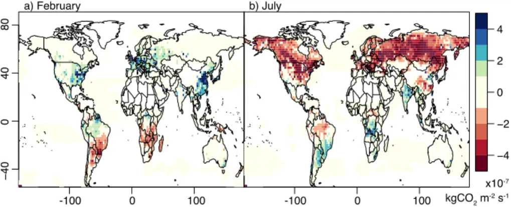
and is not part of the data assimilation. Instead, we use biospheric, oceanic, biomass burning, and fossil fuel CO2fluxes from CT (version “CT2011_oi”, Fig. 1) (Peters et al.,

2007, http://carbontracker.noaa.gov). Furthermore, we use CT as the initial condition for global atmospheric CO2 mixing ratios on 1 January and 1 May 2009. Each CAM

ensemble member uses the same initial condition for atmospheric CO2, so any

subse-10

quent differences in CO₂among the model realizations are due entirely to meteorolog-ical uncertainties.

We estimate 6 hourly CO2 transport uncertainties using the standard deviation of

CO₂ concentrations across the 64 model realizations (e.g., Fig. 2). To make this esti-mate, we calculate the standard deviation of each row inX[CO₂], where the subscript

15

“[CO2]” refers to the atmospheric CO2 concentrations estimated by the ensemble. In

addition, we characterize temporal covariance or correlation in transport errors (i.e., in X_[CO

2]). To estimate an error decorrelation time, we use a variogram analysis. In specific, we fit an exponential variogram model to afternoon-only model output (1– 7 p.m. LT) associated with a number of existing, global atmospheric CO2 observation

20

sites. Both Kitanidis (1997) and the Supplement describe variograms in greater detail. The remainder of the methods section applies this CO2 and meteorology modeling

(9)

ACPD

14, 23681–23709, 2014

S. M. Miller et al.

Title Page

Tables Figures

◭ ◮

Back Close

Full Screen / Esc

Discussion

P

a

per

|

Discus

sion

P

a

per

|

Discussion

P

a

per

|

Discussion

P

a

per

|

2.4 Case study 1: how biased would CarbonTracker fluxes need to be before that bias were detectable above CO2transport uncertainties?

In this case study, we construct a hypothesis test to determine whether biases in CT CO₂ fluxes would be detectable above atmospheric transport uncertainties. CT is a commonly-used global CO2flux estimate created by the US National Oceanic and

5

Atmospheric Administration (NOAA). To create CT, NOAA scientists use atmospheric CO₂ data from observations towers and surface sites around the world and estimate regional scaling factors that optimize an initial CO2flux model (Peters et al., 2007).

We test whether a hypothetical bias in regional scaling factors, like those estimated by CT, would be detectable at atmospheric CO₂observation sites across the globe. We 10

build this test using the CO2 sum of squared residuals (SSR) from the CAM–LETKF

model ensemble. A number of previous statistical and/or greenhouse gas studies con-struct hypothesis tests using squared residuals (e.g., Sheskin, 2003; Huntzinger et al., 2011).

In this setup, we construct the test as follows. First, compute the SSR associated 15

with the transport uncertainties:

SSR=

n2

X

H_[CO

2]X[CO2]

2

(2)

This equation interpolates the model residuals (X[CO₂]) to the observation sites, squares

these residuals, and sums them over the entire time period of interest. More specifically, 20

the variablen₂refers to the number of hourly CO₂observations at an observation site over the time span of the hypothesis test. In addition,H[CO₂] (n2×m2) is the matrix that

interpolates or maps the ensemble deviations (X[CO₂], dimensionsm2×k) to the CO2

observations. Lastly, SSR (1×k) are the sum of squared residuals from each of the kCAM–LETKF model ensemble members. Note that some of the ensemble members 25

will be closer than others to the ensemble mean or best estimate ( ¯x[CO₂]). Therefore,

(10)

ACPD

14, 23681–23709, 2014

S. M. Miller et al.

Title Page

Tables Figures

◭ ◮

Back Close

Full Screen / Esc

Discussion

P

a

per

|

Discus

sion

P

a

per

|

Discussion

P

a

per

|

Discussion

P

a

per

|

Second, we compute the SSR associated with a hypothetical bias (λ) in the fluxes:

FSSR₌

n₂

X

(_∆CO₂)2

∆CO2=λH[CO₂]

¯

x[CO₂,surface]−x¯[CO₂,600 hPa]

(3)

The output of this equation, FSSR, is a scalar that estimates the squared residuals 5

due to a biased flux estimate, summed over all observations at a given CO2

measure-ment site. The variable λ represents a hypothetical bias in CT fluxes. In this study, we conduct the hypothesis test at each measurement site individually, so the variable λ is specific to the site being considered. In addition, the variables in parentheses (x¯[CO₂,surface]−x¯[CO₂,600 hPa]) quantify the contribution of regional-scale fluxes to CO2at

10

the atmospheric observation site. Many top-down studies pre-subtract free troposphere or marine “clean air” concentrations from the CO2 measurements or model output at

the observation sites (e.g., Gerbig et al., 2003; Gourdji et al., 2012). These top-down studies then optimize regional fluxes to match the pre-subtracted CO₂ observations. In this study, we similarly subtract modeled concentrations at 600 hPa in the free tro-15

posphere (x¯[CO₂,600 hPa]) from those at the CO2 observation sites (x¯[CO₂,surface]). The

concentrations at 600 hPa are not necessarily a perfect measure of “clean air” concen-trations. Rather, this approach is an approximation similar to that used in the existing literature. This difference in concentrations is then used to estimate how a regional bias in CT fluxes would manifest at a given observation site (∆CO₂, in ppm).

20

Finally, we test the hypothesis. If the FSSR is larger than most of the k SSR asso-ciated with the meteorological uncertainties, then we can distinguish the flux bias (λ) above the meteorological noise. This statement can be formalized into a hypothesis test as follows:

A={SSR|SSR>FSSR} (4)

25

p=|A|

(11)

ACPD

14, 23681–23709, 2014

S. M. Miller et al.

Title Page

Tables Figures

◭ ◮

Back Close

Full Screen / Esc

Discussion

P

a

per

|

Discus

sion

P

a

per

|

Discussion

P

a

per

|

Discussion

P

a

per

|

whereAis the set of SSR that are greater than FSSR, and the expression|A|indicates the number of elements in A. If the p value is less than 0.05, we have disproven the null hypothesis – that the hypothetical bias (λ) in CO2fluxes is indistinguishable above

the transport uncertainties.

Note that this hypothesis test accounts for both variance and temporal covariance in 5

the CO2 transport uncertainties, a concept discussed in detail in the Supplement. In

addition, note that FSSR will almost never be zero due to diurnal or daily changes in NEP, even if the monthly-averaged NEP at a given site is zero.

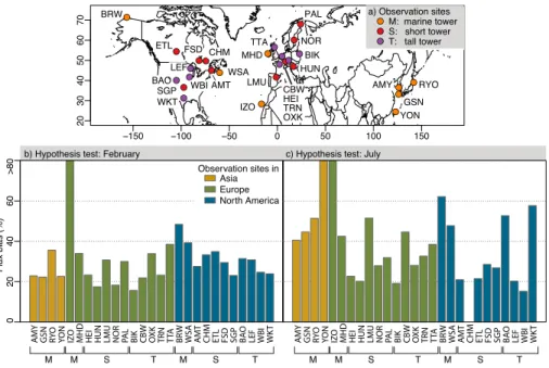
We conduct the hypothesis test above for both February and July 2009 at a variety of different observation sites in North America, Asia, and Europe. We report the results 10

of this hypothesis test for a representative selection of global CO2 observation sites

– different types of observation towers located on different continents and in different biomes. Furthermore, we test this hypothesis using month-long modeled time series corresponding to afternoon data only (1–7 p.m. LT). We use this month-long window because CO2budgets are often reported in month-long increments.

15

In summary, case study 1 quantifies the extent to which atmospheric CO₂transport errors can obscure any regional biases in estimated CO2fluxes. The next case study, in

contrast, explores the meteorological conditions under which sustained CO2transport

errors may be more likely to occur.

2.5 Case study 2: which meteorological factors may be associated with sus-20

tained, month-long transport biases?

We create a relatively simple, synthetic experiment to explore the meteorological con-ditions under which month-long model biases in atmospheric transport may occur. The spatial patterns in the CO2transport uncertainties are heavily influenced by spatial

pat-terns in the CO2fluxes (Fig. 2). In other words, regions with large fluxes or large diurnal

25

(12)

ACPD

14, 23681–23709, 2014

S. M. Miller et al.

Title Page

Tables Figures

◭ ◮

Back Close

Full Screen / Esc

Discussion

P

a

per

|

Discus

sion

P

a

per

|

Discussion

P

a

per

|

Discussion

P

a

per

|

space and time. This experiment serves as a lens to explore the possible effects of different meteorological parameters independent of the spatial variability in CO2fluxes.

To this end, we initialize CAM-LETKF runs with zero atmospheric concentration of this synthetic tracer and then run CAM-LETKF forward for one month using constant global emissions (e.g., for both February and July 2009). Any uncertainties in the at-5

mospheric distribution of this tracer are solely due to meteorological parameters, not due to the spatial distribution of the underlying fluxes.

Next, we calculate the coefficient of variation (CV) associated with the monthly-averaged surface concentrations. The CV is an inverted signal-to-noise ratio; it mea-sures the uncertainty in modeled surface concentrations relative to the average surface 10

concentration (σ_µ). For example, an uncertainty of 1 ppm in modeled concentrations is most problematic if the signal from surface fluxes is weak, and a 1 ppm uncertainty is less problematic if the signal from surface sources is strong.

For this setup, the CV equals the standard deviation in the monthly-averaged sur-face concentrations divided by the monthly sursur-face concentration averaged across all 15

64-realizations. We then plot the tracer CV against monthly-averaged meteorological parameters and their associated uncertainties from CAM–LETKF. These relationships give insight into the meteorological conditions or meteorological uncertainties that are associated with month-long biases in the modeled synthetic tracer.

3 Results and discussion 20

3.1 Uncertainties in the 6 hourly modeled CO2concentrations

Before examining the two case studies in detail, we first provide context on the CO2

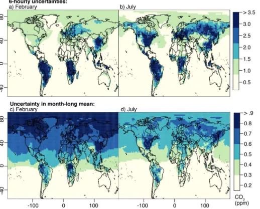
transport uncertainties estimated with CT fluxes and CAM–LETKF. Figure 2a and b visually summarize the average 6 hourly CO₂transport uncertainties (standard devia-tions) in the model surface layer; these figures show how CO₂ transport uncertainties 25

(13)

loca-ACPD

14, 23681–23709, 2014

S. M. Miller et al.

Title Page

Tables Figures

◭ ◮

Back Close

Full Screen / Esc

Discussion

P

a

per

|

Discus

sion

P

a

per

|

Discussion

P

a

per

|

Discussion

P

a

per

|

tion. Furthermore, the transport uncertainties in Fig. 2a and b show several distinctive features. The largest uncertainties are localized to regions where either the magnitude or the diurnal cycle of the CT fluxes is largest (e.g., the US Eastern Seaboard and southern Siberia during summertime, the Amazon, the Congo, and eastern China). CO₂ transport uncertainties in the Eastern US and East Asia bleed, to a smaller de-5

gree, over the adjacent ocean where surface fluxes are small.

These transport uncertainties are in the range of the uncertainties estimated in a number of previous studies. For example, the spatial patterns in the 6 hourly un-certainties are similar to those modeled by Liu et al. (2011) using CAM-LETKF and temperature-scaled CO2 fluxes from TRANSCOM 3. In addition, a number of previous

10

studies focused on the effects of perturbing individual meteorological parameters at specific observation sites or for individual aircraft campaigns (e.g., Gerbig et al., 2003, 2008; Lin and Gerbig, 2005; Kretschmer et al., 2012). Our 6 hourly transport uncer-tainties, though very different in both scope and scale, are comparable in magnitude to the individual parameter uncertainties estimated by Gerbig et al. (2003), Gerbig et al. 15

(2008), and Kretschmer et al. (2012) but are less than the uncertainties in Lin and Ger-big (2005). Furthermore, our estimated 6 hourly transport uncertainties also appear similar to or slightly smaller than the model–data mismatch errors estimated at individ-ual observation sites in several inversion studies (e.g., Peters et al., 2007; Schuh et al., 2010; Gourdji et al., 2012). Model–data mismatch includes not only transport errors but 20

also any model or data errors unrelated to an imperfect initial flux estimate. This result may reflect the fact that atmospheric transport often dominates model-data mismatch errors.

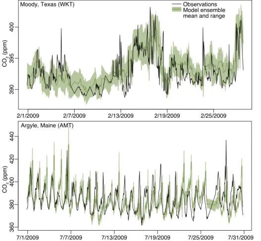
Figure 3 places these transport uncertainties in context of CO₂ data measured at two observation sites in the United States. These time series plots validate the model’s 25

capacity to simulate daily variations in CO2 concentrations. Furthermore, the

compar-ison illustrates the magnitude of the CO₂ transport uncertainties relative to the diurnal cycle in CO2concentrations. For example, the uncertainties at AMT in July are∼30 %

(14)

ACPD

14, 23681–23709, 2014

S. M. Miller et al.

Title Page

Tables Figures

◭ ◮

Back Close

Full Screen / Esc

Discussion

P

a

per

|

Discus

sion

P

a

per

|

Discussion

P

a

per

|

Discussion

P

a

per

|

in these plots usually encapsulates the hourly-averaged measurements. CT fluxes are estimated using these CO2observations and the TM5 transport model (Tracer Model,

version 5) (Peters et al., 2007), so one might expect the CAM model to fit the CO2

ob-servations relatively well. In the instances when the model ensemble does not encap-sulate the hourly-averaged CO2 measurements, one of the many other non-transport

5

error types could be to blame; the ensemble spread only encompasses transport error and does not include measurement error, error due to finite model resolution, or errors in the fluxes. The Supplement provides more example CO2 model–data comparisons,

meteorology model validation, and data assimilation diagnostics.

3.2 CO2transport uncertainties at longer time scales

10

The uncertainty in monthly-averaged CO₂ concentrations provides one measure of how transport errors persist over time. In other words, these uncertainties provide a metric of error correlations in CO2 transport. Uncorrelated transport errors will

av-erage out, to a large degree, over many model time steps, but temporal correlations prevent the errors from averaging down over time. As a result, large uncertainties 15

in monthly-averaged concentrations indicate the potential for persistent bias in CO2

fluxes estimated using atmospheric observations. Such bias could lead to under- or over-estimation of regional-scale CO₂budgets.

To this end, Fig. 2c and d displays uncertainties in the month-long average surface concentrations for February and July 2009. In contrast to the 6 hourly uncertainties, 20

these uncertainties are far more spatially-distributed; the largest uncertainties are not just associated with regions that have large fluxes. This result implies that CO2

trans-port errors are correlated over longer periods of time in remote regions, compared to regions with large anthropogenic or biospheric fluxes. Furthermore, month-long trans-port uncertainties are large across the entire Northern Hemisphere during February 25

(15)

ACPD

14, 23681–23709, 2014

S. M. Miller et al.

Title Page

Tables Figures

◭ ◮

Back Close

Full Screen / Esc

Discussion

P

a

per

|

Discus

sion

P

a

per

|

Discussion

P

a

per

|

Discussion

P

a

per

|

study discussed in that section provides insight into why the month-long uncertainties may be large across the Northern Hemisphere during winter.

A variogram analysis provides an additional measure of the error correlations in CO2transport (see Sect. 2.3 and the Supplement). Based upon this analysis, we

esti-mate CO₂transport error decorrelation times of 2.2 and 2.3 days at global atmospheric 5

CO2observation sites during February and July, respectively (see Table S1). The error

decorrelation times are generally longer at marine sites (average of 2.9 and 2.7 days in February and July, respectively) or at sites that are far from large CO2 fluxes. For

ex-ample, the longest error decorrelation times occur at coastal sites in Japan, Korea and the Canary Islands. In contrast, decorrelation times are usually shorter than average 10

for observation sites on the European mainland.

This level of temporal correlation in the CO₂ transport errors implies several large-scale conclusions for estimating CO2 fluxes. First, observation sites that are far from

large fluxes are more likely to produce a biased CO2 budget than sites near to large

surface fluxes. These “remote” sites see a lower CO₂ signal from surface fluxes, and 15

the transport errors at these locations are generally correlated over longer periods of time. Second, most existing top-down studies will underestimate the uncertainties in estimated CO₂fluxes. Existing inversions rarely account for error correlations in CO₂ transport and most likely underestimate the posterior uncertainties as a direct result. The next Sect. 3.3 quantifies the impact of the transport uncertainties discussed above 20

on surface flux estimation.

3.3 Case study 1: how biased would CT fluxes need to be before that bias were detectable above the CO2transport uncertainties?

We use a case study from CT to understand how transport errors translate into uncer-tainty in a top-down, CO₂flux estimate. In specific, if the flux scaling factors estimated 25

(16)

ACPD

14, 23681–23709, 2014

S. M. Miller et al.

Title Page

Tables Figures

◭ ◮

Back Close

Full Screen / Esc

Discussion

P

a

per

|

Discus

sion

P

a

per

|

Discussion

P

a

per

|

Discussion

P

a

per

|

Figure 4 shows the results of this case study (described in Sect. 2.4) at a selection of global CO2 observation sites. The y-axis of each bar plot shows the minimum bias

that would be detectable using hourly-averaged CO2 observations collected over an

entire month. The mean minimum detectable bias across all non-marine sites is 29 % (at a month-long time scale). The results are not substantially different at short versus 5

tall non-marine tower sites: 27 % and 31 %, respectively. In other words, the tall towers examined in this analysis are neither more or less sensitive to biased CO₂ fluxes in comparison to the set of short towers in Fig. 4. At marine sites, in contrast, the minimum detectable bias is far larger: 76 % on average.

These results show a number of additional trends across the different observation 10

sites. In general, towers that are near large sources are better able to detect bias in the modeled fluxes. These include observation sites in the central and eastern US or in Germany and Eastern Europe – sites that are strongly influence by terrestrial (ver-sus marine) airflow relative to other locations. Most of these towers see large signals from biospheric fluxes during summer (Figs. S9–S14). Other towers, in contrast, are 15

less sensitive to detecting bias during the summertime (e.g., the marine towers and towers in the western US). The western US towers, for example, are surrounded by weak biosphere uptake that is diluted into a larger mixed layer during summer. But during summer, transport uncertainties increase due to large seasonal fluxes in adja-cent regions. The sensitivity of the marine Japanese and Korean sites also declines 20

in the summer. At these sites, the signal from surface fluxes is largest in winter. Dur-ing summer, biosphere uptake somewhat cancels the signal from large anthropogenic emissions in China.

Note that this analysis only considers uncertainties due to meteorology. The capa-bilities of the atmospheric observations would deteriorate if other errors were included 25

(17)

ACPD

14, 23681–23709, 2014

S. M. Miller et al.

Title Page

Tables Figures

◭ ◮

Back Close

Full Screen / Esc

Discussion

P

a

per

|

Discus

sion

P

a

per

|

Discussion

P

a

per

|

Discussion

P

a

per

|

3.4 Case study 2: which meteorological factors are associated with sustained, month-long atmospheric transport biases?

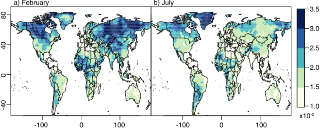
We now examine the results of the synthetic tracer experiment (Sect. 2.5) to uncover possible drivers of atmospheric transport biases.

Figure 5 displays the coefficient of variation (CV) for monthly-averaged surface con-5

centrations of the synthetic tracer. The CV, a unitless quantity, does not just indicate where the uncertainties are largest. Rather, the CV indicates the magnitude of these uncertainties relative to the mean modeled tracer concentration. Arguably, this noise-to-signal ratio measures the influence of transport uncertainties more effectively than a simple standard deviation. The remainder of this section focuses only on land regions 10

because most existing top-down studies focus on land fluxes.

This coefficient shows a number of distinctive seasonal and spatial patterns. Like the uncertainties in monthly-averaged CO₂ (Fig. 2c and d), the CV in Fig. 5 is highest in boreal and arctic regions of the Northern Hemisphere during winter. The CV is lowest over Europe, Australia, and the Amazon during all seasons.

15

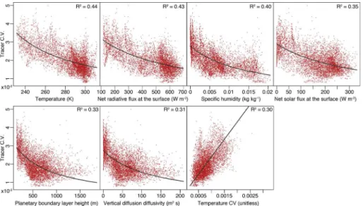
We plot the synthetic tracer CV against numerous modeled meteorological param-eters to understand the possible drivers behind the transport uncertainties. Of the 60 variables tested (Table S2), seven of the variables showed correlations (R2) with the tracer CV that are greater or equal to 0.3 (Fig. 6). Meteorological conditions that lead to high atmospheric stability and low energy are most closely associated with persis-20

tent tracer uncertainties (relative to mean surface concentrations). For example, a high tracer CV is associated with low temperatures, low net radiative flux, low net solar flux, low planetary boundary layer height, and low vertical diffusion diffusivity. Furthermore, many of the meteorological variables exhibit a nonlinear relationship with the tracer CV; the CV increases more quickly when net radiation and planetary boundary heights are 25

low.

(18)

ACPD

14, 23681–23709, 2014

S. M. Miller et al.

Title Page

Tables Figures

◭ ◮

Back Close

Full Screen / Esc

Discussion

P

a

per

|

Discus

sion

P

a

per

|

Discussion

P

a

per

|

Discussion

P

a

per

|

higher in regions with consistent low energy, limited vertical mixing, and/or high albedo. These biases are unlikely to be represented by most existing inversion uncertainty calculations, as explained in the previous sections. Furthermore, the meteorological model ensemble is not necessarily more uncertain these regions (see Figs. S16 and S17). Note that month-long CO2 transport biases did not correlate as strongly with

5

meteorology uncertainties. Rather, the extent to which meteorological uncertainties translate into tracer transport uncertainties appears to depend, at least in part, on the stability and net energy input associated with the boundary layer.

4 Conclusions

In this paper, we use two case studies to investigate the potential for bias in top-down 10

CO2flux estimates due to errors in modeled atmospheric CO2transport. The first case

study examines the ability of in situ atmospheric observations to detect bias in esti-mated CO₂ fluxes. Among other results, we find that CT would need to be biased by 29 %, on average, before that bias were detectable above CO2transport uncertainties

at terrestrial, atmospheric observation sites. These results are strongly influenced by 15

temporal correlations in the transport uncertainties. In other words, atmospheric CO₂ measurements contain less information about the fluxes than is usually assumed by top-down studies that overlook transport error covariances. As a result, most existing inversions are likely to underestimate the uncertainties in estimated CO₂fluxes and/or may be vulnerable to unforeseen biases in the estimated fluxes. Accounting for these 20

correlated errors can be as simple as modifying one of the covariance matrix inputs in a Bayesian inversion. Accordingly, this study provides information to improve the setup of future top-down inverse modeling studies – an improvement that will widen the confidence interval on the estimated fluxes.

In a subsequent case study, we investigate the factors associated with month-long 25

(19)

at-ACPD

14, 23681–23709, 2014

S. M. Miller et al.

Title Page

Tables Figures

◭ ◮

Back Close

Full Screen / Esc

Discussion

P

a

per

|

Discus

sion

P

a

per

|

Discussion

P

a

per

|

Discussion

P

a

per

|

mospheric transport are not only localized to regions with large fluxes. Rather, these biases may be more likely to occur at observation sites that are far from large fluxes and in regions with high atmospheric stability and low net radiation. Existing top-down flux studies may be more likely to estimate inaccurate regional fluxes under those con-ditions.

5

The Supplement related to this article is available online at doi:10.5194/acpd-14-23681-2014-supplement.

Acknowledgements. This work was conducted at the Department of Energy’s (DOE) Lawrence

Berkeley National Laboratory as part of a DOE Computational Science Graduate Fellowship. The research used resources of the National Energy Research Scientific Computing Center,

10

which is supported by the DOE’s Office of Science under Contract No. DE-AC02-05CH11231. CarbonTracker CT2011_oi results are provided by NOAA ESRL, Boulder, Colorado, USA from the website at http://carbontracker.noaa.gov. We thank Steven Wofsy for his feedback on the manuscript and thank Ed Dlugokencky of NOAA.

References 15

Baker, D. F., Law, R. M., Gurney, K. R., Rayner, P., Peylin, P., Denning, A. S., Bousquet, P., Bruhwiler, L., Chen, Y.-H., Ciais, P., Fung, I. Y., Heimann, M., John, J., Maki, T., Maksyu-tov, S., Masarie, K., Prather, M., Pak, B., Taguchi, S., and Zhu, Z.: TransCom 3 inversion intercomparison: impact of transport model errors on the interannual variability of regional CO₂fluxes, 1988–2003, Global Biogeochem. Cy., 20, GB1002, doi:10.1029/2004GB002439,

20

2006. 23684

Chen, H., Zhou, T., Neale, R. B., Wu, X., and Zhang, G. J.: Performance of the New NCAR CAM3.5 in East Asian Summer Monsoon simulations: sensitivity to modifications of the con-vection scheme, J. Climate, 23, 3657–3675, doi:10.1175/2010JCLI3022.1, 2010. 23686 Ciais, P., Rayner, P., Chevallier, F., Bousquet, P., Logan, M., Peylin, P., and Ramonet, M.:

At-25

(20)

ACPD

14, 23681–23709, 2014

S. M. Miller et al.

Title Page

Tables Figures

◭ ◮

Back Close

Full Screen / Esc

Discussion

P

a

per

|

Discus

sion

P

a

per

|

Discussion

P

a

per

|

Discussion

P

a

per

|

Gas Inventories, edited by: Jonas, M., Nahorski, Z., Nilsson, S., and Whiter, T., Springer, the Netherlands, doi:10.1007/978-94-007-1670-4_6, 69–92, 2011. 23684

Collins, W. D., Bitz, C. M., Blackmon, M. L., Bonan, G. B., Bretherton, C. S., Carton, J. A., Chang, P., Doney, S. C., Hack, J. J., Henderson, T. B., Kiehl, J. T., Large, W. G., McKenna, D. S., Santer, B. D., and Smith, R. D.: The community climate system model

ver-5

sion 3 (CCSM3)., J. Climate, 19, 2122–2143, doi:10.1175/JCLI3761.1, 2006. 23686

Enting, I.: Inverse Problems in Atmospheric Constituent Transport, Cambridge Atmospheric and Space Science Series, Cambridge University Press, Cambridge, 2002. 23683

Gerbig, C., Lin, J. C., Wofsy, S. C., Daube, B. C., Andrews, A. E., Stephens, B. B., Bakwin, P. S., and Grainger, C. A.: Toward constraining regional-scale fluxes of CO₂with atmospheric

ob-10

servations over a continent: 2. Analysis of COBRA data using a receptor-oriented frame-work, J. Geophys. Res.-Atmos., 108, 4757, doi:10.1029/2003jd003770, 2003. 23684, 23690, 23693

Gerbig, C., Körner, S., and Lin, J. C.: Vertical mixing in atmospheric tracer transport models: error characterization and propagation, Atmos. Chem. Phys., 8, 591–602,

doi:10.5194/acp-15

8-591-2008, 2008. 23684, 23693

Gourdji, S. M., Mueller, K. L., Yadav, V., Huntzinger, D. N., Andrews, A. E., Trudeau, M., Petron, G., Nehrkorn, T., Eluszkiewicz, J., Henderson, J., Wen, D., Lin, J., Fischer, M., Sweeney, C., and Michalak, A. M.: North American CO₂exchange: inter-comparison of mod-eled estimates with results from a fine-scale atmospheric inversion, Biogeosciences, 9, 457–

20

475, doi:10.5194/bg-9-457-2012, 2012. 23683, 23690, 23693

Gurney, K. R., Law, R. M., Denning, A. S., Rayner, P. J., Baker, D., Bousquet, P., Bruhwiler, L., Chen, Y. H., Cials, P., Fan, S., Fung, I. Y., Gloor, M., Heimann, M., Higuchi, K., John, J., Maki, T., Maksyutov, S., Masarie, K., Peylin, P., Prather, M., Pak, B. C., Randerson, J., Sarmiento, J., Taguchi, S., Takahashi, T., and Yuen, C. W.: Towards robust regional

esti-25

mates of CO₂sources and sinks using atmospheric transport models, Nature, 415, 626–630, doi:10.1038/415626a, 2002. 23683, 23684

Hunt, B. R., Kalnay, E., Kostelich, E. J., Ott, E., Patil, D. J., Sauer, T., Szunyogh, I., Yorke, J. A., and Zimin, A. V.: Four-dimensional ensemble Kalman filtering, Tellus A, 56, 273–277, doi:10.1111/j.1600-0870.2004.00066.x, 2004. 23686, 23688

30

(21)

ACPD

14, 23681–23709, 2014

S. M. Miller et al.

Title Page

Tables Figures

◭ ◮

Back Close

Full Screen / Esc

Discussion

P

a

per

|

Discus

sion

P

a

per

|

Discussion

P

a

per

|

Discussion

P

a

per

|

Huntzinger, D. N., Gourdji, S. M., Mueller, K. L., and Michalak, A. M.: The utility of continuous atmospheric measurements for identifying biospheric CO₂ flux variability, J. Geophys. Res.-Atmos., 116, D06110, doi:10.1029/2010JD015048, 2011. 23689

Huntzinger, D., Post, W., Wei, Y., Michalak, A., West, T., Jacobson, A., Baker, I., Chen, J., Davis, K., Hayes, D., Hoffman, F., Jain, A., Liu, S., McGuire, A., Neilson, R., Potter, C.,

Poul-5

ter, B., Price, D., Raczka, B., Tian, H., Thornton, P., Tomelleri, E., Viovy, N., Xiao, J., Yuan, W., Zeng, N., Zhao, M., and Cook, R.: North American Carbon Program (NACP) regional in-terim synthesis: terrestrial biospheric model intercomparison, Ecol. Model., 232, 144–157, doi:10.1016/j.ecolmodel.2012.02.004, 2012. 23683

Kanamitsu, M., Ebisuzaki, W., Woollen, J., Yang, S.-K., Hnilo, J. J., Fiorino, M., and

Pot-10

ter, G. L.: NCEP–DOE AMIP-II reanalysis (R-2), B. Am. Meteorol. Soc., 83, 1631–1643, doi:10.1175/BAMS-83-11-1631, 2002. 23687

Kitanidis, P. K.: Introduction to Geostatistics: Applications in Hydrogeology, Stanford-Cambridge program, Cambridge University Press, Cambridge, 1997. 23688

Kretschmer, R., Gerbig, C., Karstens, U., and Koch, F.-T.: Error characterization of CO₂vertical

15

mixing in the atmospheric transport model WRF-VPRM, Atmos. Chem. Phys., 12, 2441– 2458, doi:10.5194/acp-12-2441-2012, 2012. 23684, 23693

Kretschmer, R., Gerbig, C., Karstens, U., Biavati, G., Vermeulen, A., Vogel, F., Hammer, S., and Totsche, K. U.: Impact of optimized mixing heights on simulated regional atmospheric trans-port of CO₂, Atmos. Chem. Phys., 14, 7149–7172, doi:10.5194/acp-14-7149-2014, 2014.

20

23684

Lauvaux, T., Pannekoucke, O., Sarrat, C., Chevallier, F., Ciais, P., Noilhan, J., and Rayner, P. J.: Structure of the transport uncertainty in mesoscale inversions of CO₂ sources and sinks using ensemble model simulations, Biogeosciences, 6, 1089–1102, doi:10.5194/bg-6-1089-2009, 2009. 23684

25

Li, H., Kalnay, E., and Miyoshi, T.: Simultaneous estimation of covariance inflation and ob-servation errors within an ensemble Kalman filter, Q. J. Roy. Meteor. Soc., 135, 523–533, doi:10.1002/qj.371, 2009. 23687, 23688

Lin, J. C. and Gerbig, C.: Accounting for the e_ffect of transport errors on tracer inversions, Geophys. Res. Lett., 32, L01802, doi:10.1029/2004GL021127, 2005. 23684, 23693

30

(22)

ACPD

14, 23681–23709, 2014

S. M. Miller et al.

Title Page

Tables Figures

◭ ◮

Back Close

Full Screen / Esc

Discussion

P

a

per

|

Discus

sion

P

a

per

|

Discussion

P

a

per

|

Discussion

P

a

per

|

Liu, J., Fung, I., Kalnay, E., Kang, J.-S., Olsen, E. T., and Chen, L.: Simultaneous assimilation of AIRS XCO₂and meteorological observations in a carbon climate model with an ensemble Kalman filter, J. Geophys. Res.-Atmos., 117, D05309, doi:10.1029/2011JD016642, 2012. 23685, 23687

Michalak, A., Bruhwiler, L., and Tans, P.: A geostatistical approach to surface flux

5

estimation of atmospheric trace gases, J. Geophys. Res.-Atmos., 109, D14109, doi:10.1029/2003JD004422, 2004. 23683

Michalak, A. M., Hirsch, A., Bruhwiler, L., Gurney, K. R., Peters, W., and Tans, P. P.: Maximum likelihood estimation of covariance parameters for Bayesian atmospheric trace gas surface flux inversions, J. Geophys. Res.-Atmos., 110, D24107, doi:10.1029/2005JD005970, 2005.

10

23684

Miyoshi, T.: The Gaussian approach to adaptive covariance inflation and its implementa-tion with the local ensemble transform Kalman filter, Mon. Weather Rev., 139, 1519–1535, doi:10.1175/2010MWR3570.1, 2011. 23687, 23688

Oleson, K. W., Niu, G.-Y., Yang, Z.-L., Lawrence, D. M., Thornton, P. E., Lawrence, P. J.,

15

Stöckli, R., Dickinson, R. E., Bonan, G. B., Levis, S., Dai, A., and Qian, T.: Improvements to the Community Land Model and their impact on the hydrological cycle, J. Geophys. Res.-Biogeo., 113, G01021, doi:10.1029/2007JG000563, 2008. 23686

Parazoo, N. C., Denning, A. S., Kawa, S. R., Pawson, S., and Lokupitiya, R.: CO₂flux estimation errors associated with moist atmospheric processes, Atmos. Chem. Phys., 12, 6405–6416,

20

doi:10.5194/acp-12-6405-2012, 2012. 23684

Peters, W., Jacobson, A. R., Sweeney, C., Andrews, A. E., Conway, T. J., Masarie, K., Miller, J. B., Bruhwiler, L. M. P., Petron, G., Hirsch, A. I., Worthy, D. E. J., Werf, G. R. v. d., Rander-son, J. T., Wennberg, P. O., Krol, M. C., and Tans, P. P.: An atmospheric perspective on North American carbon dioxide exchange: CarbonTracker, Proceedings of the National Academy

25

of Sciences, with updates documented at: http://carbontracker.noaa.gov (last access: 12 September 2014), 104, 18925–18930, doi:10.1073/pnas.0708986104, 2007. 23683, 23688, 23689, 23693, 23694

Pino, D., Vilà-Guerau de Arellano, J., Peters, W., Schröter, J., van Heerwaarden, C. C., and Krol, M. C.: A conceptual framework to quantify the influence of convective boundary

30

(23)

ACPD

14, 23681–23709, 2014

S. M. Miller et al.

Title Page

Tables Figures

◭ ◮

Back Close

Full Screen / Esc

Discussion

P

a

per

|

Discus

sion

P

a

per

|

Discussion

P

a

per

|

Discussion

P

a

per

|

Raczka, B. M., Davis, K. J., Huntzinger, D., Neilson, R. P., Poulter, B., Richardson, A. D., Xiao, J., Baker, I., Ciais, P., Keenan, T. F., Law, B., Post, W. M., Ricciuto, D., Schaefer, K., Tian, H., Tomelleri, E., Verbeeck, H., and Viovy, N.: Evaluation of continental carbon cycle simulations with North American flux tower observations, Ecol. Monogr., 83, 531–556, doi:10.1890/12-0893.1, 2013. 23683

5

Schuh, A. E., Denning, A. S., Corbin, K. D., Baker, I. T., Uliasz, M., Parazoo, N., Andrews, A. E., and Worthy, D. E. J.: A regional high-resolution carbon flux inversion of North America for 2004, Biogeosciences, 7, 1625–1644, doi:10.5194/bg-7-1625-2010, 2010. 23693

Sheskin, D.: Handbook of Parametric and Nonparametric Statistical Procedures, 3 edn., Taylor and Francis, Boca Raton, Florida, 2003. 23689

10

Stephens, B. B., Gurney, K. R., Tans, P. P., Sweeney, C., Peters, W., Bruhwiler, L., Ciais, P., Ramonet, M., Bousquet, P., Nakazawa, T., Aoki, S., Machida, T., Inoue, G., Vinnichenko, N., Lloyd, J., Jordan, A., Heimann, M., Shibistova, O., Langenfelds, R. L., Steele, L. P., Francey, R. J., and Denning, A. S.: Weak northern and strong tropical land carbon uptake from vertical profiles of atmospheric CO₂, Science, 316, 1732–1735,

15

doi:10.1126/science.1137004, 2007. 23684

(24)

ACPD

14, 23681–23709, 2014

S. M. Miller et al.

Title Page

Tables Figures

◭ ◮

Back Close

Full Screen / Esc

Discussion

P

a

per

|

Discus

sion

P

a

per

|

Discussion

P

a

per

|

Discussion

P

a

per

|

−40 0 40 80

−4 −2 0 2 4

-100 0 100 -100 0 100

a) February b) July

kgCO₂ m-2_s-1

x10-7

(25)

ACPD

14, 23681–23709, 2014

S. M. Miller et al.

Title Page

Tables Figures

◭ ◮

Back Close

Full Screen / Esc

Discussion

P

a

per

|

Discus

sion

P

a

per

|

Discussion

P

a

per

|

Discussion

P

a

per

|

Figure 2.The top panels display average 6 hourly CO₂ transport uncertainties estimated by CAM–LETKF. The uncertainties (standard deviations) are for the surface model layer for(a)

(26)

ACPD

14, 23681–23709, 2014

S. M. Miller et al.

Title Page

Tables Figures

◭ ◮

Back Close

Full Screen / Esc

Discussion

P

a

per

|

Discus

sion

P

a

per

|

Discussion

P

a

per

|

Discussion

P

a

per

|

CO

2

(ppm)

390

395

400

Moody, Texas (WKT) Observations

Model ensemble mean and range

2/1/2009 2/7/2009 2/13/2009 2/19/2009 2/25/2009

CO

2

(ppm)

360

380

400

420

440

Argyle, Maine (AMT)

7/1/2009 7/7/2009 7/13/2009 7/19/2009 7/25/2009 7/31/2009

(27)

ACPD

14, 23681–23709, 2014

S. M. Miller et al.

Title Page Abstract Introduction Conclusions References Tables Figures ◭ ◮ ◭ ◮ Back Close

Full Screen / Esc

Printer-friendly Version Interactive Discussion Discussion P a per | Discus sion P a per | Discussion P a per | Discussion P a per |

b) Hypothesis test: February c) Hypothesis test: July

A

MY

GSN RY

O

Y

ON

IZ

O

MHD HEI HUN LMU NOR PAL BIK CB

W

O

XK

TRN TT

A

BR

W

WSA AM

T

CHM ETL FSD SGP BA

O

LEF WBI WK

T

A

MY

GSN RY

O

Y

ON

IZ

O

MHD HEI HUN LMU NOR PAL BIK CB

W

O

XK

TRN TT

A

BR

W

WSA AM

T

CHM ETL FSD SGP BA

O

LEF WBI WK

T

M M S T M S T

Flux bias (%)

0

20

40

60

>80 Observation sites in Asia Europe North America

M M S T M S T

−150 −100 −50 0 50 100 150

20 30 40 50 60 70

a) Observation sites M: marine tower S: short tower T: tall tower BRW ETL FSD CHM GSN WSA IZO AMT LEF BAO SGP WKT WBI YON RYO AMY BIK HUN PAL NOR MHD TTA LMU CBW HEI TRN OXK

(28)

ACPD

14, 23681–23709, 2014

S. M. Miller et al.

Title Page

Tables Figures

◭ ◮

Back Close

Full Screen / Esc

Discussion

P

a

per

|

Discus

sion

P

a

per

|

Discussion

P

a

per

|

Discussion

P

a

per

|

1.0 1.5 2.0 2.5 3.0 3.5

x10-2

a) February b) July

-100 0 100 -100 0 100

-40 0

40

80

(29)

ACPD

14, 23681–23709, 2014

S. M. Miller et al.

Title Page

Tables Figures

◭ ◮

Back Close

Full Screen / Esc

Discussion

P

a

per

|

Discus

sion

P

a

per

|

Discussion

P

a

per

|

Discussion

P

a

per

|

Figure 6.Each panel shows the correlation between the synthetic tracer CV (Fig. 5) and various monthly-averaged meteorological parameters estimated by CAM-LETKF. We test the correla-tion with 60 different parameters (Table S2) and plot the relationships for whichR2≥0.3. In all cases, we fit both a standard major axis regression and nonlinear least squares ( 1

[β1×parameter+β2])