Consistency of long-term elemental carbon trends from thermal and optical measurements in the IMPROVE network

(1)

AMTD

5, 3837–3859, 2012

Carbon trends from thermal and optical measurements in the

IMPROVE network

L.-W. A. Chen et al.

Title Page Abstract Introduction Conclusions References

Tables Figures

◭ ◮

Back Close

Full Screen / Esc

Printer-friendly Version Interactive Discussion

Discussion

P

a

per

|

Dis

cussion

P

a

per

|

Discussion

P

a

per

|

Discussio

n

P

a

per

|

Atmos. Meas. Tech. Discuss., 5, 3837–3859, 2012 www.atmos-meas-tech-discuss.net/5/3837/2012/ doi:10.5194/amtd-5-3837-2012

Atmospheric Measurement Techniques Discussions

This discussion paper is/has been under review for the journal Atmospheric Measurement Techniques (AMT). Please refer to the corresponding final paper in AMT if available.

Consistency of long-term elemental

carbon trends from thermal and optical

measurements in the IMPROVE network

L.-W. A. Chen1,2, J. C. Chow1,2, J. G. Watson1,2, and B. A. Schichtel3

1

Division of Atmospheric Sciences, Desert Research Institute, 2215 Raggio Parkway, Reno, Nevada, 89512, USA

2

State Key Laboratory of Loess and Quaternary Geology, Institute of Earth Environment, Chinese Academy of Sciences, 10 Fenghui South Road, Xi’an, 710075, China

3

Cooperative Institute for Research in the Atmosphere, Colorado State University, 1375 Campus Delivery, Fort Collins, Colorado, 80523, USA

Received: 14 April 2012 – Accepted: 8 May 2012 – Published: 31 May 2012 Correspondence to: L.-W. A. Chen ([email protected])

(2)

AMTD

5, 3837–3859, 2012

IMPROVE network

Tables Figures

◭ ◮

Back Close

Full Screen / Esc

Discussion

P

a

per

|

Dis

cussion

P

a

per

|

Discussion

P

a

per

|

Discussio

n

P

a

per

|

Abstract

Decreasing trends of elemental carbon (EC) have been reported at US Interagency Monitoring of Protected Visual Environments (IMPROVE) network since 1990, consis-tent with the phase-in of cleaner engines, residential biomass burning technologies, and prescribed burning methods. The EC trends from the past decade are cautioned

5

due to an upgrade of IMPROVE carbon analyzers and the thermal/optical analysis pro-tocol since 2005. Filter reflectance (τ_R) values measured as part of the carbon analysis were retrieved from archived data and compared with EC for 65 sites with more com-plete records from 2000 to 2009. The EC-τR relationships show only minor changes

of EC quantified by the original and upgraded instruments for most of the IMPROVE

10

samples. EC andτRshow universal decreasing trends across the US. The EC andτR

trends are correlated well, with national average downward trends of 4.5 % and 4.1 % (of the 2000–2004 baseline medians) per year, respectively. The consistency between independent EC andτR trends adds to the weight-of-evidence that EC reductions are

real rather than an artifact of the measurement process.

15

1 Introduction

Elemental carbon (EC), also known as black carbon (BC) or light-absorbing carbon (LAC), is the dominant aerosol component that absorbs visible radiation in the tropo-sphere (Andreae and Gelencser, 2006). EC aerosols from incomplete fuel combustion are non-spherical and internally mixed with organic carbon (OC) (Chakrabarty et al.,

20

2006a,b). Jacobson (2009) estimates the 100-yr Global Warming Potential (GWP) of EC+OC from fossil- and bio-fuel combustion to be 800–1300 relative to carbon diox-ide (CO₂). Reducing EC emissions could be a short-term and cost-e_ffective method for slowing global warming (Jacobson, 2002; Bond and Sun, 2005), as well as providing co-benefits for public health, visibility, and material damage (Chow and Watson, 2011).

(3)

AMTD

5, 3837–3859, 2012

IMPROVE network

Tables Figures

◭ ◮

Back Close

Full Screen / Esc

Discussion

P

a

per

|

Dis

cussion

P

a

per

|

Discussion

P

a

per

|

Discussio

n

P

a

per

|

Long-term monitoring of aerosol chemical composition in the Interagency Monitoring of Protected Visual Environments (IMPROVE) network (Watson, 2002) reveals a de-creasing trend in average EC concentrations by over 25 % in the US from 1990 to 2004 (Murphy et al., 2011) as well as decreases of 40–60 % EC for urban and non-urban California sites from 1988 to 2007 (Bahadur et al., 2011a,b; Schichtel et al., 2011).

5

These trends are consistent with emission reduction measures implemented to attain PM2.5and PM10 National Ambient Air Quality Standards for residential wood

combus-tion (Hough and Kowalczyk, 1983; Butler, 1988; Hough et al., 1988), prescribed burn-ing (Riebau and Fox, 2001; Tian et al., 2008), and engine exhaust (Lloyd and Cackette, 2001). Even though IMPROVE data were available through 2009, Murphy et al. (2011)

10

chose to exclude data from 2005 onward owing to potential biases that might be caused by an upgrade in IMPROVE carbon analyzers beginning in 2005. Chow et al. (2007) demonstrated equivalence between measurements made with the original (Chow et al., 1993) and upgraded (Chow et al., 2007, 2011) analyzers for hundreds of samples from a variety of environments. However, average EC concentrations and EC/OC

ra-15

tios increased at some (but not all) IMPROVE sites from 2004 to 2005, as illustrated in Fig. 1. The objective of this study is to investigate the recent (2000–2009) trends in IMPROVE EC along with those of filter reflectance which serves as an independent surrogate for EC.

The IMPROVE thermal/optical reflectance (TOR) analysis protocol separates EC

20

from OC on filter samples by temperature-dependent volatilization and oxidation. EC is defined as carbon that does not evolve at∼580◦C in an inert helium (He) atmosphere and is subsequently oxidized to CO₂ with the introduction of oxygen (2 %) at higher temperatures, up to 840◦C. A fraction of OC chars in the inert atmosphere, as evi-denced by decreases in light (633 nm He-Ne laser) reflected from the aerosol deposit

25

(4)

AMTD

5, 3837–3859, 2012

IMPROVE network

Tables Figures

◭ ◮

Back Close

Full Screen / Esc

Discussion

P

a

per

|

Dis

cussion

P

a

per

|

Discussion

P

a

per

|

Discussio

n

P

a

per

|

usually white, similar to the appearance of a blank filter. Non-white filters occasionally occur during dust events, and these are flagged as part of the IMPROVE protocol.

The 2005 carbon analyzer upgrade led to a transition from the IMPROVE to IM-PROVE A protocol. The transition did not change the temperatures plateaus but rather reflected “actual” analysis temperatures that had been implemented since the

incep-5

tion of the IMPROVE network (Chow et al., 2005). The replacement analyzer allows for more precise sample positioning and temperature control, more flexible data acquisi-tion, a higher intensity laser light beam, and lower trace oxygen levels in the inert He atmosphere than did the old analyzer design. It also allows simultaneous monitoring of filter reflectance and transmittance. Since 2005, light transmitted through the filter and

10

aerosol deposit as well as that reflected from the deposit has been used for charring correction. Thermal/optical transmittance (TOT) often reports higher POC and lower EC than TOR. Chen et al. (2004) and Chow et al. (2004) attributed this to charring of organic vapors adsorbed within the filter (Watson et al., 2009; Chow et al., 2010) which attenuate transmittance substantially but have a minor effect on reflectance from the

15

surface deposit.

Optical measurements designed for charring correction provide alternatives for quan-tifying EC or BC abundances on filters. Filter attenuation using reflected light (τR) or

transmitted light (τT) is defined as:

τR=−ln R/R0

20

τT=−ln T/T0

(1)

whereR0 and T0 are reflectance and transmittance of blank filters, respectively, and

R and T are reflectance and transmittance of particle-laden filters (prior to carbon analysis), respectively. τ_R or τ_T can be a practically linear function of the light

ab-25

sorption coefficient (babs) for filter samples (Lindberg et al., 1999; Quincey, 2007). The

widely-deployed aethalometer and particle-soot absorption photometer (PSAP) esti-mate babs from τT which is then converted to BC using assumed mass absorption

(5)

AMTD

5, 3837–3859, 2012

IMPROVE network

Tables Figures

◭ ◮

Back Close

Full Screen / Esc

Discussion

P

a

per

|

Dis

cussion

P

a

per

|

Discussion

P

a

per

|

Discussio

n

P

a

per

|

references therein).babs and BC based on τR are also reported (e.g., Edwards et al.,

1983; Janssen et al., 2011).τRcould be more variable in estimatingbabs thanτTsince

the angular distribution of reflectance is more sensitive to the chemical composition of particle deposits (Kopp et al., 1999; Petzold and Sch ¨onlinner, 2004). Nonlinearity amongbabs (or BC), τR, and τT increases with higher loading samples (Arnott et al.,

5

2005) though it was shown in Chen et al. (2004) that the linear relationship between reflectance and transmittance holds up to an EC loading equivalent to ∼20 µg cm−2 on a filter or∼2 µg m−3in ambient air for IMPROVE network samples (32.7 m3 of air sampled through a 3.53 cm2filter area).

Since τ_R, essentially a measurement of the darkness of the filter deposit, was

10

recorded for every IMPROVE sample before, during, and after the analyzer upgrade and is not related to the thermal/optical analysis, it can be used as an independent in-dicator of EC. Investigating the EC andτRrelationship before and after the upgrade is

necessary. This relationship should be site-, and possibly season-specific, considering the diverse environments represented by IMPROVE samples. Furthermore,τR trends

15

provide an additional verification for observed EC trends.

2 Methodology

Digital thermograms (which record 1 s value for reflectance, temperature, and carbon content) for>83 000 IMPROVE samples acquired by 24-h sampling on every third day from CY2000 through CY2009 were reprocessed to obtain the initial (dark aerosol

de-20

posit) and final (white filter) reflectance values. Data recovery varied by site; typically exceeding 92 % for 2005–2009, but ≤80 % for 2000–2004 due to deteriorating stor-age media (floppy disks and CD-ROMs; it was not practical to recover data from the paper documentation). The 65 sites with the longest records and highest data recov-ery rates are listed in Table 1 and used for subsequent analysis. Each of these sites

25

(6)

AMTD

5, 3837–3859, 2012

IMPROVE network

Tables Figures

◭ ◮

Back Close

Full Screen / Esc

Discussion

P

a

per

|

Dis

cussion

P

a

per

|

Discussion

P

a

per

|

Discussio

n

P

a

per

|

from a ten-second average of the initial and final reflectance for all samples. The final reflectance represents e_ffectiveR0as all EC has been removed from the filter.

Pre- and post-upgradeτR at a particular IMPROVE site are related to EC through a

linear model:

[EC]−=c− +b− ×[τR]−

5

[EC]₊=c₊ +b₊ ×[τR]₊ (2)

where brackets indicate column vectors of EC orτR including all pre (−)/post (+)

up-grade (on 1 January 2005) data, andcandbare regression coefficients (c: intercept; b: slope).candbare expected to differ (i.e.,c₊₌6 c−and/orb₊6=b−) only if the

instru-10

ment upgrade introduced a bias in EC that is substantially larger than typical measure-ment uncertainties. To examine the changes in b and c, Eqs. (3) and (4) are nested into:

_[EC] −

[EC]₊

=c− _I

I

+ ∆c

_O

I

+b− _[τ

R]−

[τR]₊

+ ∆b

_O

[τR]+

(3)

whereI _and O _{are unit and zero column vectors and} _∆_c_and _∆_b _represents _c

+−c−

15

and b₊−b−, respectively. Meaningful changes in cand b would lead to ∆c and ∆b

that di_ffer from zero at a statistically-significant level (Gujarati, 1970a,b). A robust least-squares regression method that lowers the influence of outliers was applied to deter-mine the coefficients and respective standard errors and p-values in Eq. (5). This is achieved by the Matlab® robustfit function with the Huber iterative reweighting

algo-20

rithm (Dutter and Huber, 1981).

Statistical consistency of c and b pre- and post-2005 (i.e., non-significant ∆c and

∆b) result from relatively small∆c and∆bor large standard errors. The latter would suggest an insu_fficient correlation between EC andτRforτRto be a good predictor for

EC. Therefore, it is important to investigate the regression’s correlation coefficient as

25

(7)

AMTD

5, 3837–3859, 2012

IMPROVE network

Tables Figures

◭ ◮

Back Close

Full Screen / Esc

Discussion

P

a

per

|

Dis

cussion

P

a

per

|

Discussion

P

a

per

|

Discussio

n

P

a

per

|

[EC]− concentration). ∆c/EC−med provides a better evaluation of changes in ∆cthan

∆c/c− since c− is usually small to near zero. Lower and Thompson (1988) show that

[EC]₊ can be related to [EC]−by solving Eqs. (3) and (4) aftercandbare determined.

This relationship would be the best estimate for determining the relationship between [EC]₊ and [EC]−, given that a direct regression is not possible.

5

EC andτRtrends were further assessed using a non-parametric Mann-Kendall (M-K)

test (Kendall, 1975; Yue et al., 2002) which examines the sign of slopes for all possible data pairs and determines trend significance from the difference in positive and nega-tive signs. All data acquired in the same year are considered as concurrent measure-ments (ties) in the test to minimize influence of intra-annual trends such as seasonal

10

variations (Salas, 1993). M-K statistics yield Sen’s slope (Sen, 1968; Burn and Hag El-nur, 2002), which is the median slope across all possible data pairs, and its p-value and confidence intervals. Sen’s slope provides a more quantitative estimate of the trends. M-K statistics were calculated with Matlab® code provided by Burkey (2009).

3 Results and discussion

15

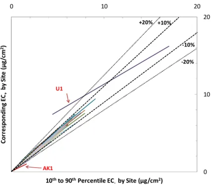
The majority of correlation coefficients (r) of EC versus τ_R from Eq. (5) exceed 0.8 (Table S-1, Supplement). Lower r is found for Urban, Appalachia, and Ohio River Valley sites with high EC concentrations, especially Washington D.C. (U1 in Fig. 2;r=0.59) and James River Face Wilderness (A1, r=0.67). Thirty-six of the 65 sites show no changes in regression slope prior to and after 2005 at the 5 % significance level (i.e.,

20

p(∆b)>0.05). Thirty-four of the thirty-six sites, including all Appalachia sites, show no significant changes in regression intercept prior to and after 2005 (i.e.,p(∆c)>0.05). p(∆c) for the remaining two sites (Cape Romain NWR [SE3] and Canyonlands NP [CP6], see Table 1/Fig. 2), though <0.05, are still >0.01 (1 % significant level). The absolute values of∆band∆cfor these 36 sites are small, generally within 10 % ofb−

25

(8)

AMTD

5, 3837–3859, 2012

IMPROVE network

Tables Figures

◭ ◮

Back Close

Full Screen / Esc

Discussion

P

a

per

|

Dis

cussion

P

a

per

|

Discussion

P

a

per

|

Discussio

n

P

a

per

|

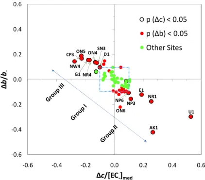
The other 29 sites are separated into two groups according to Fig. 3. One group (Group II) exhibits negative ∆b along with positive ∆c. Six sites of Group II have both ∆b and ∆c that are significantly different from zero (p <0.05), including Brig-antine NWR (E1), U1, Lostwood (NP3), UL Bend (NP6), Glacier NP (NR1), and De-nali NP (AK1). These sites are located in eastern (E1, U1) and northern states (NP3,

5

NP6, NR1, AK1). The other group (Group III) exhibits positive∆band mostly negative

∆c. Group III contains 8 sites with both ∆b and ∆c significantly different from zero (p <0.05), including White Pass [NW4], Three Sisters Wilderness [ON4], Mount Hood [ON5], Bliss SP [SN3], Death Valley [D1], Great Basin [G1], Hance Camp at Grand Canyon NP [CP3], and Bridger Wilderness [NR4]), all of which are located in the

West-10

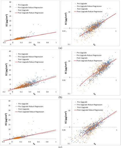
ern Cordillera of the continental US (Fig. 2). Figure 4 shows examples of EC-τRscatter

for these groups.

The POC fraction generally increased for samples analyzed beginning in 2005 due to higher purity of the inert He atmosphere and new procedures to assure that purity (Chow et al., 2007, 2011). Even with the reflectance correction, some POC can be

15

mis-classified as EC, thereby increasing the EC fraction. This is more evident when EC/POC ratios are low and would likely move the EC-τR regression towards a higher

intercept and lower-to-unchanged slope. Figure 3 is not consistent with this effect being dominant, except possibly at a few Group II sites including E1 (exemplified in Fig. 4b).

For Group III samples, low EC values tend to be even lower beginning in 2005 for

20

the same τR (e.g., Fig. 4c). The reason for this is unclear, though it might be related

to different sensitivities of reflectance measurements between the old and new instru-ments for low EC levels. The opposite e_ffects apparent in Group II and Group III could occur simultaneously and to some extent cancel each other. To test whether extreme EC values due to special events such as wildfires can bias the robust regression,

re-25

(9)

AMTD

5, 3837–3859, 2012

IMPROVE network

Tables Figures

◭ ◮

Back Close

Full Screen / Esc

Discussion

P

a

per

|

Dis

cussion

P

a

per

|

Discussion

P

a

per

|

Discussio

n

P

a

per

|

Since regression slopes increase or decrease when intercepts decrease or increase (i.e., change in opposite direction), EC₊may shift higher or lower compared to EC−

de-pending on site and EC loading. Figure 5 shows, by site, the characteristic EC₊vs. EC−

relationships between the 10th and 90th EC−concentration percentiles, which contains

80 % of the samples. The linear relationships were derived from Eqs. (3) and (4) by

5

eliminating the common variable τR, as suggested by Lower and Thompson (1988).

EC₊ is shown to be within±10 % of EC− for the most part. Larger deviations, e.g., 10–

20 % or−10–−20 %, are seen for EC−≤3 µg cm −2

. Two extreme outliers are U1 and AK1, which represent the highest and lowest EC IMPROVE environments, respectively. There may be some change in the EC responses of the old and new instruments for

10

high and low extremes.

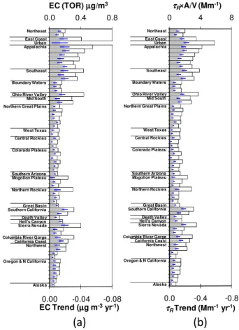
The robust M-K test confirms decreasing trends of EC from 2000 through 2009 (Fig. 6), with the largest and smallest rate observed at one Appalachia (A2: −0.021 µg m−3yr−1) site and one Central Rockies (CR2: −0.003 µg m−3yr−1) site, re-spectively. The trends are statistically significant for all 65 sites at the 5 % significance

15

level. This implies 1.3–8.3 % reductions of ambient EC each year (scaled to EC−med

as 2000–2004 is the IMPROVE baseline period). The national average trend, as cal-culated from the percentage trends weighted by EC−medat each site, would be−4.5 %

per year. With a simple unweighted regression, Fig. S-1 (Supplement) shows median EC decreasing at 3–5 % per year from 2000–2009. Murphy et al. (2011) report a lower

20

value,∼ −2.2 % EC per year, for March 1990–February 2004. Their analysis was based on average rather than median EC concentrations.

Figure 6 also shows significantly decreasing trends (p <0.05) for τR at all except

one site in the Northwest (NW4, White Pass, Washington) where the p-value for the negativeτR trend (−0.099 Mm

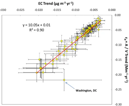
−1

yr−1) is 0.051. The EC andτR trends are highly

cor-25

related, atr2=0.9 and slope=10 m2g−1(Fig. 7). Washington, DC (U1 site), the only urban site in this dataset, is an outlier where the EC₊ seems much higher than EC−

based on reflectance (Fig. 5), leading to a smaller EC trend than expected from theτR

(10)

AMTD

5, 3837–3859, 2012

IMPROVE network

Tables Figures

◭ ◮

Back Close

Full Screen / Esc

Discussion

P

a

per

|

Dis

cussion

P

a

per

|

Discussion

P

a

per

|

Discussio

n

P

a

per

|

for other urban sites. The national averageτRtrend, as scaled toτR−medis−4.1 % per

year, also consistent with the national EC trend.

Although subtle changes are found between EC-τRrelationships pre- and post-2005,

the consistency between recent EC andτR trends for the majority of IMPROVE sites

do not support that such changes have introduced a major or common bias for the

5

EC trends. Environmental changes, probably due to changing EC emissions and year-to-year meteorological variability, are of larger magnitude than measurement method changes. EC concentrations appear to continue decreasing beyond the 1990–2004 period examined by Murphy et al. (2011) at an average rate of 4.1–4.5 % per year. The Regional Haze Rule (U.S. EPA, 1999) has set the goal of returning visibility to natural

10

conditions by 2064. For EC, the natural concentrations are estimated to be∼10 % of the 2000–2004 baseline period. At the current rate of progess, this goal should be met by the 2064 deadline.

Supplementary material related to this article is available online at: http://www.atmos-meas-tech-discuss.net/5/3837/2012/

15

amtd-5-3837-2012-supplement.pdf.

Acknowledgements. This work was sponsored in part by the National Park Service IMPROVE Carbon Analysis Contract No. C2350000894, and the US. EPA task number T2350086187. The conclusions are those of the authors and do not necessarily reflect the views of the sponsoring agencies.

(11)

AMTD

5, 3837–3859, 2012

IMPROVE network

Tables Figures

◭ ◮

Back Close

Full Screen / Esc

Discussion

P

a

per

|

Dis

cussion

P

a

per

|

Discussion

P

a

per

|

Discussio

n

P

a

per

|

References

Andreae, M. O. and Gelencs ´er, A.: Black carbon or brown carbon? The nature of light-absorbing carbonaceous aerosols, Atmos. Chem. Phys., 6, 3131–3148, doi:10.5194/acp-6-3131-2006, 2006.

Arnott, W. P., Hamasha, K., Moosm ¨uller, H., Sheridan, P. J., and Ogren, J. A.: Towards aerosol

5

light-absorption measurements with a 7-wavelength Aethalometer: Evaluation with a photoa-coustic instrument and 3-wavelength nephelometer, Aerosol Sci. Tech., 39, 17–29, 2005. Bahadur, R., Feng, Y., Russell, L. M., and Ramanathan, V.: Impact of California’s air pollution

laws on black carbon and their implications for direct radiative forcing, Atmos. Environ., 45, 1162–1167, 2011a.

10

Bahadur, R., Feng, Y., Russell, L. M., and Ramanathan, V.: Response to comments on “Impact of California’s air pollution laws on black carbon and their implications for direct radiative forcing” by R. Bahadur et al., Atmos. Environ., 45, 4119–4121, 2011b.

Bond, T. C. and Sun, H. L.: Can reducing black carbon emissions counteract global warming?, Environ. Sci. Technol., 39, 5921–5926, 2005.

15

Burkey, J.: Mann-Kendall Tau-b with Sen’s Method (enhanced Mat-lab code), http://www.mathworks.com/matlabcentral/fileexchange/ 11190-mann-kendall-tau-b-with-sens-method-enhanced (last access: 28 May 2012), 2009.

Burn, D. H. and Hag Elnur, M. A.: Detection of hydrologic trends and variability, J. Hydrol., 255,

20

107–122, 2002.

Butler, A. T.: Control of woodstoves by state regulation as a fine particulate control strategy, in: Transactions, PM₁₀: Implementation of Standards, edited by: Mathai, C. V. and Stonefield, D. H., Air Pollution Control Association, Pittsburgh, PA, 654–663, 1988.

Chakrabarty, R. K., Moosm ¨uller, H., Arnott, W. P., Garro, M. A., and Walker, J.: Structural and

25

fractal properties of particles emitted from spark ignition engines, Environ. Sci. Technol., 40, 6647–6654, 2006a.

Chakrabarty, R. K., Moosm ¨uller, H., Garro, M. A., Arnott, W. P., Walker, J., Susott, R. A., Babbitt, R. E., Wold, C. E., Lincoln, E. N., and Hao, W. M.: Emissions from the laboratory combustion of wildland fuels: Particle morphology and size, J. Geophys. Res.-Atmos., 111, D07204,

30

(12)

AMTD

5, 3837–3859, 2012

IMPROVE network

Tables Figures

◭ ◮

Back Close

Full Screen / Esc

Discussion

P

a

per

|

Dis

cussion

P

a

per

|

Discussion

P

a

per

|

Discussio

n

P

a

per

|

Chen, L.-W. A., Chow, J. C., Watson, J. G., Moosm ¨uller, H., and Arnott, W. P.: Modeling re-flectance and transmittance of quartz-fiber filter samples containing elemental carbon parti-cles: Implications for thermal/optical analysis, J. Aerosol Sci., 35, 765–780, 2004.

Chow, J. C. and Watson, J. G.: Air quality management of multiple pollutants and multiple effects, Air Qual. Clim. Change J., 45, 26–32, 2011.

5

Chow, J. C., Watson, J. G., Pritchett, L. C., Pierson, W. R., Frazier, C. A., and Purcell, R. G.: The DRI Thermal/Optical Reflectance carbon analysis system: Description, evaluation and applications in U.S. air quality studies, Atmos. Environ., 27A, 1185–1201, 1993.

Chow, J. C., Watson, J. G., Chen, L.-W. A., Arnott, W. P., Moosm ¨uller, H., and Fung, K. K.: Equivalence of elemental carbon by Thermal/Optical Reflectance and Transmittance with

10

different temperature protocols, Environ. Sci. Technol., 38, 4414–4422, 2004.

Chow, J. C., Watson, J. G., Chen, L.-W. A., Paredes-Miranda, G., Chang, M.-C. O., Trimble, D., Fung, K. K., Zhang, H., and Zhen Yu, J.: Refining temperature measures in thermal/optical carbon analysis, Atmos. Chem. Phys., 5, 2961–2972, doi:10.5194/acp-5-2961-2005, 2005. Chow, J. C., Watson, J. G., Chen, L.-W. A., Chang, M. C. O., Robinson, N. F., Trimble, D. L.,

15

and Kohl, S. D.: The IMPROVE A temperature protocol for thermal/optical carbon analysis: Maintaining consistency with a long-term database, J. Air Waste Manage. Assoc., 57, 1014– 1023, 2007.

Chow, J. C., Watson, J. G., Chen, L.-W. A., Rice, J., and Frank, N. H.: Quantification of PM_2.5 organic carbon sampling artifacts in US networks, Atmos. Chem. Phys., 10, 5223–5239,

20

doi:10.5194/acp-10-5223-2010, 2010.

Chow, J. C., Watson, J. G., Robles, J., Wang, X. L., Chen, L.-W. A., Trimble, D. L., Kohl, S. D., Tropp, R. J., and Fung, K. K.: Quality assurance and quality control for thermal/optical analysis of aerosol samples for organic and elemental carbon, Anal. Bioanal. Chem., 401, 3141–3152, 2011.

25

Dutter, R. and Huber, P. J.: Numerical methods for the non linear robust regression problem, J. Stat. Comput. Simul., 13, 79–113, 1981.

Edwards, J. D., Ogren, J. A., Weiss, R. E., and Charlson, R. J.: Particulate air pollutants: A comparison of British “Smoke” with optical absorption coe_fficients and elemental carbon con-centration, Atmos. Environ., 17, 2337–2341, 1983.

30

(13)

AMTD

5, 3837–3859, 2012

IMPROVE network

Tables Figures

◭ ◮

Back Close

Full Screen / Esc

Discussion

P

a

per

|

Dis

cussion

P

a

per

|

Discussion

P

a

per

|

Discussio

n

P

a

per

|

Gujarati, D.: Use of dummy variables in testing for equality between sets of coefficients in two linear regressions: A note, Am. Stat., 24, 50–52, 1970b.

Hough, M. L. and Kowalczyk, J. F.: A comprehensive strategy to reduce residential wood burn-ing impacts in small urban communities, J. Air Poll. Control Assoc., 33, 1121–1125, 1983. Hough, M. L., Tombleson, B., and Wolgamott, M.: Oregon approach to reducing residential

5

woodsmoke as part of the PM₁₀ strategy, in: Transactions, PM₁₀: Implementation of Stan-dards, edited by: Mathai, C. V. and Stonefield, D. H., Air Pollution Control Association, Pitts-burgh, PA, 646–653, 1988.

Jacobson, M. Z.: Control of fossil-fuel particulate black carbon plus organic matter, possi-bly the most effective method of slowing global warming, J. Geophys. Res., 107, 4410,

10

doi:10.1029/2001JD001376, 2002.

Jacobson, M. Z.: Testimony for U.S. Environmental Protection Agency Public Hearing on the Proposed Endangerment and Cause or Contribute Findings for Greenhouse Gases Under the Clean Air Act, http://www.stanford.edu/group/efmh/jacobson/PDF%20files/ EPAEndang0509.pdf (last access: 28 May 2012), 18 May 2009.

15

Janssen, N. A. H., Hoek, G., Simic-Lawson, M., Fischer, P., van Bree, L., Ten Brink, H., Keuken, M., Atkinson, R. W., Anderson, H. R., Brunekreef, B., and Cassee, F. R.: Black carbon as an additional indicator of the adverse health effects of airborne particles compared with PM₁₀ and PM_2.5, Environ. Health Perspect., 119, 1691–1699, 2011.

Kendall, M. G.: Rank Correlation Methods, Griffin, London, UK, 1975.

20

Kopp, C., Petzold, A., and Niessner, R.: Investigation of the specific attenuation cross-section of aerosols deposited on fiber filters with a polar photometer to determine black carbon, J. Aerosol Sci., 30, 1153–1163, 1999.

Lindberg, J. D., Douglass, R. E., and Garvey, D. M.: Atmospheric particulate absorption and black carbon measurement, Appl. Optics, 38, 2369–2376, 1999.

25

Lloyd, A. C. and Cackette, T. A.: Critical review – Diesel engines: Environmental impact and control, J. Air Waste Manage. Assoc., 51, 809–847, 2001.

Lower, W. R. and Thompson, W. A.: An indirect test of correlation, Environ. Toxicol. Chem., 7, 77–80, 1988.

Murphy, D. M., Chow, J. C., Leibensperger, E. M., Malm, W. C., Pitchford, M., Schichtel, B. A.,

30

(14)

AMTD

5, 3837–3859, 2012

IMPROVE network

Tables Figures

◭ ◮

Back Close

Full Screen / Esc

Discussion

P

a

per

|

Dis

cussion

P

a

per

|

Discussion

P

a

per

|

Discussio

n

P

a

per

|

Petzold, A. and Sch ¨onlinner, M.: Multi-angle absorption photometry – A new method for the measurement of aerosol light absorption and atmospheric black carbon, J. Aerosol Sci., 35, 421–441, 2004.

Quincey, P. G.: A relationship between Black Smoke Index and Black Carbon concentration, Atmos. Environ., 41, 7964–7968, 2007.

5

Riebau, A. R. and Fox, D.: The new smoke management, Inter. J. Wildland Fire, 10, 415–427, 2001.

Salas, J. D.: Analysis and modeling of hydrologic time series, in: Handbook of Hydrology, edited by: Maidment, D. R., McGraw-Hill, Columbus, OH, 19.1–19.63, 1993.

Schichtel, B. A., Pitchford, M. L., and White, W. H.: Comments on “Impact of California’s Air

10

Pollution Laws on Black Carbon and their Implications for Direct Radiative Forcing” by R. Ba-hadur et al., Atmos. Environ., 45, 4116–4118, 2011.

Sen, P. K.: Estimates of the regression coefficient based on Kendall’s tau, J. Amer. Stat. Assoc., 63, 1379–1389, 1968.

Tian, D., Wang, Y. H., Bergin, M., Hu, Y. T., Liu, Y. Q., and Russell, A. G.: Air quality impacts

15

from prescribed forest fires under di_fferent management practices, Environ. Sci. Technol., 42, 2767–2772, 2008.

U.S. EPA: 40 CFR Part 51 – Regional haze regulations: Final rule, Federal Register, Environ-mental Protection Agency, Washington, DC, 64, 35714–35774, 1999.

Watson, J. G.: Visibility: Science and regulation – 2002 Critical Review, J. Air Waste Manage.

20

Assoc., 52, 628–713, 2002.

Watson, J. G., Chow, J. C., and Chen, L.-W. A.: Summary of organic and elemental car-bon/black carbon analysis methods and intercomparisons, Aerosol Air Qual. Res., 5, 65–102, 2005.

Watson, J. G., Chow, J. C., Chen, L.-W. A., and Frank, N. H.: Methods to assess carbonaceous

25

aerosol sampling artifacts for IMPROVE and other long-term networks, J. Air Waste Manage. Assoc., 59, 898–911, 2009.

(15)

AMTD

5, 3837–3859, 2012

IMPROVE network

Tables Figures

◭ ◮

Back Close

Full Screen / Esc

Discussion

P

a

per

|

Dis

cussion

P

a

per

|

Discussion

P

a

per

|

Discussio

n

P

a

per

|

Table 1.Region, location, and data completeness (2000–2009) of EC andτRfor 65 IMPROVE sites selected for this study.

Location Data completeness∗

Regions Code Name Class I area Latitude Longitude m.s.l. (m) 2000–2004 2005–2009

Northeast NE1 MOOS1 Moosehorn NWR 45.1259 −67.2661 77 73 % 97 %

NE2 ACAD1 Acadia NP 44.3771 −68.261 157 78 % 99 %

East Coast E1 BRIG1 Brigantine NWR 39.465 −74.4492 5 80 % 95 %

Urban U1 WASH1 Washington D.C. 38.8762 −77.0344 15 71 % 93 %

Appalachia A1 JARI1 James River Face Wilderness 37.6266 −79.5125 289 72 % 99 %

A2 SIPS1 Sipsy Wilderness 34.3433 −87.3388 286 72 % 92 %

A3 GRSM1 Great Smoky Mountains NP 35.6334 −83.9416 810 73 % 98 %

A4 LIGO1 Linville Gorge 35.9723 −81.9331 968 72 % 93 %

A5 SHEN1 Shenandoah NP 38.5229 −78.4348 1079 73 % 97 %

A6 DOSO1 Dolly Sods Wilderness 39.1053 −79.4261 1182 74 % 100 %

Southeast SE1 CHAS1 Chassahowitzka NWR 28.7484 −82.5549 4 77 % 95 %

SE2 OKEF1 Okefenokee NWR 30.7405 −82.1283 48 80 % 98 %

SE3 ROMA1 Cape Romain NWR 32.941 −79.6572 4 77 % 97 %

Boundary waters B1 SENE1 Seney 46.2889 −85.9503 214 75 % 97 %

B2 ISLE1 Isle Royale NP 47.4596 −88.1491 182 78 % 96 %

B3 VOYA1 Voyageurs NP #1 48.4132 −92.8303 425 71 % 92 %

Ohio River valley O1 MACA1 Mammoth Cave NP 37.1318 −86.1479 235 75 % 99 %

Mid south MS1 UPBU1 Upper Buffalo Wilderness 35.8258 −93.203 722 70 % 95 %

MS2 CACR1 Caney Creek 34.4544 −94.1429 683 72 % 93 %

Northern Great Plains NP1 WICA1 Wind Cave 43.5576 −103.484 1296 71 % 93 %

NP2 THRO1 Theodore Roosevelt 46.8948 −103.378 852 70 % 97 %

NP3 LOST1 Lostwood 48.6419 −102.402 696 76 % 91 %

NP4 MELA1 Medicine Lake 48.4871 −104.476 606 70 % 96 %

NP5 BADL1 Badlands NP 43.7435 −101.941 736 74 % 99 %

NP6 ULBE1 UL Bend 47.5823 −108.72 891 75 % 95 %

West Texas W1 BIBE1 Big Bend NP 29.3027 −103.178 1066 70 % 94 %

W2 GUMO1 Guadalupe Mountains NP 31.833 −104.809 1672 78 % 96 %

Central Rockies CR1 ROMO2 Rocky Mountain NP 40.2783 −105.546 2760 74 % 98 %

CR2 GRSA1 Great Sand Dunes NM 37.7249 −105.519 2498 76 % 93 %

CR3 WHRI1 White River NF 39.1536 −106.821 3413 76 % 96 %

Colorado Plateau CP1 BRCA1 Bryce Canyon NP 37.6184 −112.174 2481 74 % 95 %

CP2 BAND1 Bandelier NM 35.7797 −106.266 1988 76 % 94 %

CP3 HANC1 Hance Camp at Grand Canyon NP 35.9731 −111.984 2267 75 % 96 %

CP4 WEMI1 Weminuche Wilderness 37.6594 −107.8 2750 75 % 99 %

CP5 MEVE1 Mesa Verde NP 37.1984 −108.491 2172 72 % 96 %

CP6 CANY1 Canyonlands NP 38.4587 −109.821 1798 71 % 93 %

Southern Arizona SA1 CHIR1 Chiricahua NM 32.0094 −109.389 1554 70 % 95 %

Mogollon Plateau MP1 SYCA1 Sycamore Canyon 35.1406 −111.969 2046 70 % 94 %

MP2 IKBA1 Ike’s Backbone 34.3405 −111.683 1297 74 % 97 %

(16)

AMTD

5, 3837–3859, 2012

IMPROVE network

Tables Figures

◭ ◮

Back Close

Full Screen / Esc

Discussion

P

a

per

|

Dis

cussion

P

a

per

|

Discussion

P

a

per

|

Discussio

n

P

a

per

|

Table 1.Continued.

Location Data completeness∗

Regions Code Name Class I area Latitude Longitude m.s.l. (m) 2000–2004 2005–2009

Northern Rockies NR1 GLAC1 Glacier NP 48.5105 −113.997 975 74 % 94 %

NR2 MONT1 Monture 47.1222 −113.154 1282 70 % 96 %

NR3 CABI1 Cabinet Mountains 47.9549 −115.671 1441 71 % 95 %

NR4 BRID1 Bridger Wilderness 42.9749 −109.758 2626 78 % 94 %

Great Basin G1 GRBA1 Great Basin NP 39.0052 −114.216 2065 70 % 96 %

Southern California SC1 SAGO1 San Gorgonio Wilderness 34.1939 −116.913 1726 71 % 98 %

SC2 JOSH1 Joshua Tree NP 34.0695 −116.389 1235 74 % 95 %

Death Valley D1 DEVA1 Death Valley NP 36.5089 −116.848 130 70 % 96 %

Hell’s Canyon H1 STAR1 Starkey 45.2249 −118.513 1259 74 % 98 %

Sierra Nevada SN1 SEQU1 Sequoia NP 36.4894 −118.829 519 72 % 96 %

SN2 YOSE1 Yosemite NP 37.7133 −119.706 1603 75 % 94 %

SN3 BLIS1 Bliss SP (TRPA) 38.9761 −120.103 2130 71 % 93 %

Columbia River Gorge CG1 CORI1 Columbia River Gorge 45.6644 −121.001 178 76 % 96 %

California Coast CC1 PINN1 Pinnacles NM 36.4833 −121.157 302 72 % 97 %

Northwest NW1 MORA1 Mount Rainier NP 46.7583 −122.124 439 75 % 93 %

NW2 SNPA1 Snoqualmie Pass 47.422 −121.426 1049 73 % 97 %

NW3 NOCA1 North Cascades 48.7316 −121.065 568 70 % 94 %

NW4 WHPA1 White Pass 46.6243 −121.388 1827 75 % 95 %

Oregon & ON1 KALM1 Kalmiopsis 42.552 −124.059 80 80 % 98 %

Northern ON2 CRLA1 Crater Lake NP 42.8958 −122.136 1996 70 % 94 %

California ON3 LABE1 Lava Beds NM 41.7117 −121.507 1459 70 % 95 %

ON4 THSI1 Three Sisters Wilderness 44.291 −122.043 885 74 % 98 %

ON5 MOHO1 Mount Hood 45.2888 −121.784 1531 78 % 97 %

ON6 REDW1 Redwood NP 41.5608 −124.084 243 70 % 94 %

Alaska AK1 DENA1 Denali NP 63.7233 −148.968 658 75 % 96 %

(17)

AMTD

5, 3837–3859, 2012

IMPROVE network

Title Page Abstract Introduction Conclusions References Tables Figures ◭ ◮ ◭ ◮ Back Close

Full Screen / Esc

Printer-friendly Version Interactive Discussion Discussion P a per | Dis cussion P a per | Discussion P a per | Discussio n P a per | 0 0.2 0.4 0.6 0.8 1 0 0.5 1 1.5 1 9 8 9 1 9 9 0 1 9 9 1 1 9 9 2 1 9 9 3 1 9 9 4 1 9 9 5 1 9 9 6 1 9 9 7 1 9 9 8 1 9 9 9 2 0 0 0 2 0 0 1 2 0 0 2 2 0 0 3 2 0 0 4 2 0 0 5 2 0 0 6 2 0 0 7 2 0 0 8 2 0 0 9 E C /T C R a ti o E C a n d O C ( µ g m -3) Year

EC OC EC/TC

(a) 0 0.2 0.4 0.6 0.8 1 0 1 2 3 4 1 9 8 9 1 9 9 0 1 9 9 1 1 9 9 2 1 9 9 3 1 9 9 4 1 9 9 5 1 9 9 6 1 9 9 7 1 9 9 8 1 9 9 9 2 0 0 0 2 0 0 1 2 0 0 2 2 0 0 3 2 0 0 4 2 0 0 5 2 0 0 6 2 0 0 7 2 0 0 8 2 0 0 9 E C /T C R a ti o E C a n d O C ( µ g m -3) Year

EC OC EC/TC

(b) 0 0.2 0.4 0.6 0.8 1 0 0.5 1 1.5 1 9 8 9 1 9 9 0 1 9 9 1 1 9 9 2 1 9 9 3 1 9 9 4 1 9 9 5 1 9 9 6 1 9 9 7 1 9 9 8 1 9 9 9 2 0 0 0 2 0 0 1 2 0 0 2 2 0 0 3 2 0 0 4 2 0 0 5 2 0 0 6 2 0 0 7 2 0 0 8 2 0 0 9 E C /T C R a ti o E C a n d O C ( µ g m -3) Year

EC OC EC/TC

(c)

(18)

AMTD

5, 3837–3859, 2012

IMPROVE network

Tables Figures

◭ ◮

Back Close

Full Screen / Esc

Discussion

P

a

per

|

Dis

cussion

P

a

per

|

Discussion

P

a

per

|

Discussio

n

P

a

per

|

NE1 NE2

E1 U1

A1

A2

A3 A4

A5 A6

SE1 SE2

SE3 B1

B2 B3

O1

MS1 MS2 NP1

NP2 NP3 NP4

NP5 NP6

W1 W2

CR1

CR2 CR3 CP1

CP2 CP3

CP4 CP5 CP6

SA1 MP1

MP2 MP3 NR1

NR2 NR3

NR4

G1

SC1_SC2

D1 H1

SN1 SN2 SN3

CG1

CC1

NW1NW2

NW3

NW4

ON1 ON2 ON3 ON4

ON5

ON6

AK1

(19)

AMTD

5, 3837–3859, 2012

IMPROVE network

Tables Figures

◭ ◮

Back Close

Full Screen / Esc

Discussion

P

a

per

|

Dis

cussion

P

a

per

|

Discussion

P

a

per

|

Discussio

n

P

a

per

|

-0.6 -0.4 -0.2 0.0 0.2 0.4 0.6

Δ

b

/

b

-Δc/[EC_-]_med

p (Δc) < 0.05

p (Δb) < 0.05

Other Sites

U1 E1

AK1 NR1 NP3 NP6 NW4

ON5 CP3

G1 NR4 ON4SN3_D1

ON6

Fig. 3.Changes in EC-τRrobust regression intercept (∆c)/slope (∆b) relative to median EC (EC₋_med)/regression slope (b−) prior to 2005. Red: significant change in slope; solid edge:

sig-nificant change in intercept; green: all other sites without sigsig-nificant changes. Group I consists of 36 sites with∆bnot significantly different from zero. Group II consists of 17 sites with nega-tive∆bthat are significantly different from zero, and Group III consists of 12 sites with positive

(20)

AMTD

5, 3837–3859, 2012

IMPROVE network

Title Page Abstract Introduction Conclusions References Tables Figures ◭ ◮ ◭ ◮ Back Close

Full Screen / Esc

Printer-friendly Version Interactive Discussion Discussion P a per | Dis cussion P a per | Discussion P a per | Discussio n P a per | -5 0 5 10 15 20 25 30 35 40

-0.2 0 0.2 0.4 0.6 0.8 1

E C ( µ g /c m 2) τ_R Pre-Upgrade

Pre-Upgrade Robust Regression Post-Upgrade

Post-Upgrade Robust Regression

0.1 1 10

0.01 0.1 1

(a) -5 0 5 10 15 20 25 30 35 40

-0.2 0 0.2 0.4 0.6 0.8 1

0.1 1 10

0.01 0.1 1

(b) -5 0 5 10 15 20 25 30 35 40

-0.2 0 0.2 0.4 0.6 0.8 1

0.1 1 10

0.01 0.1 1

(c)

(21)

AMTD

5, 3837–3859, 2012

IMPROVE network

Tables Figures

◭ ◮

Back Close

Full Screen / Esc

Discussion

P

a

per

|

Dis

cussion

P

a

per

|

Discussion

P

a

per

|

Discussio

n

P

a

per

|

0 10 20

C

o

rr

e

sp

o

n

d

in

g

E

C+

b

y

S

it

e

(

µ

g

/c

m

2)

10th_{to 90}th_{Percentile EC}

-by Site (µg/cm2)

-20% -10% +10% +20%

U1

AK1

Fig. 5.EC₊(after upgrade) vs. EC−(before upgrade) relationships derived from robust

regres-sion analysis throughτ_R. Relationships of EC₊ and EC− with τR are determined separately, and then EC₊ is related to EC− by eliminating τR in simultaneous equations. Each solid line represents one of the 65 sites stretching from 10th to 90th percentile of EC−. Dashed lines

(22)

AMTD

5, 3837–3859, 2012

IMPROVE network

Tables Figures

◭ ◮

Back Close

Full Screen / Esc

Discussion

P

a

per

|

Dis

cussion

P

a

per

|

Discussion

P

a

per

|

Discussio

n

P

a

per

|

-0.08 -0.04 0.00

0.0 0.4 0.8

Northeast East Coast Urban Appalachia

Southeast Boundary Waters Ohio River Valley Mid South Northern Great Plains

West Texas Central Rockies Colorado Plateau

Southern Arizona Mogollon Plateau Northern Rockies

Great Basin Southern California Death Valley Hell's Canyon Sierra Nevada Columbia River Gorge California Coast Northwest

Oregon & N California

Alaska

EC Trend (µµµµg m-3_yr-1₎

EC (TOR) µµµµg/m3

-0.8 -0.4 0.0

0 4 8

Northeast East Coast Urban Appalachia

Southeast Boundary Waters Ohio River Valley Mid South Northern Great Plains

West Texas Central Rockies Colorado Plateau

Southern Arizona Mogollon Plateau Northern Rockies

Great Basin Southern California Death Valley Hell's Canyon Sierra Nevada Columbia River Gorge California Coast Northwest

Oregon & N California

Alaska

τ τ τ

τRTrend (Mm-1yr-1)

τ τ τ

τR×A/V (Mm-1)

(a) (b)

(23)

AMTD

5, 3837–3859, 2012

IMPROVE network

Tables Figures

◭ ◮

Back Close

Full Screen / Esc

Discussion

P

a

per

|

Dis

cussion

P

a

per

|

Discussion

P

a

per

|

Discussio

n

P

a

per

|

y = 10.05x + 0.01 R² = 0.90

-0.30 -0.25 -0.20 -0.15 -0.10 -0.05 0.00

-0.030 -0.025 -0.020 -0.015 -0.010 -0.005 0.000

τ

R

×

A

/

V

T

re

n

d

(M

m

-1

y

r

-1

)

EC Trend (µg m-3_yr-1₎

Washington, DC

Fig. 7.A comparison of EC and τ_R trends for 65 IMPROVE sites during 2000–2009. Aand