www.atmos-meas-tech.net/6/565/2013/ doi:10.5194/amt-6-565-2013
© Author(s) 2013. CC Attribution 3.0 License.
Atmospheric
Measurement
Techniques
Geoscientiic
Geoscientiic
Geoscientiic
Geoscientiic
Improvements to the retrieval of tropospheric NO
2
from satellite –
stratospheric correction using SCIAMACHY limb/nadir matching
and comparison to Oslo CTM2 simulations
A. Hilboll1, A. Richter1, A. Rozanov1, Ø. Hodnebrog2,*, A. Heckel3,1, S. Solberg4, F. Stordal2, and J. P. Burrows1
1Institute of Environmental Physics, University of Bremen, P.O. Box 330 440, 28334 Bremen, Germany 2University of Oslo, Oslo, Norway
3Department of Geography, Swansea University, Swansea, UK 4Norwegian Institute for Air Research, Kjeller, Norway
*now at: Center for International Climate and Environmental Research-Oslo (CICERO), Oslo, Norway
Correspondence to:A. Hilboll ([email protected])
Received: 12 June 2012 – Published in Atmos. Meas. Tech. Discuss.: 23 July 2012 Revised: 6 December 2012 – Accepted: 18 January 2013 – Published: 1 March 2013
Abstract.Satellite measurements of atmospheric trace gases
have proved to be an invaluable tool for monitoring the Earth system. When these measurements are to be used for as-sessing tropospheric emissions and pollution, as for exam-ple in the case of nadir measurements of nitrogen dioxide (NO2), it is necessary to separate the stratospheric from the tropospheric signal.
The SCIAMACHY instrument offers the unique oppor-tunity to combine its measurements in limb- and nadir-viewing geometries into a tropospheric data product, using the limb measurements of the stratospheric NO2abundances to correct the nadir measurements’ total columns.
In this manuscript, we present a novel approach to limb/nadir matching, calculating one stratospheric NO2 value from limb measurements for every single nadir mea-surement, abandoning global coverage for the sake of spatial accuracy. For comparison, modelled stratospheric NO2 columns from the Oslo CTM2 are also evaluated for stratospheric correction.
Our study shows that stratospheric NO2 columns from SCIAMACHY limb measurements very well reflect strato-spheric conditions. The zonal variability of the stratostrato-spheric NO2 field is captured by our matching algorithm, and the quality of the resulting tropospheric NO2columns improves considerably. Both stratospheric datasets need to be adjusted to the level of the nadir measurements, because a time- and latitude-dependent bias to the measured nadir columns can be observed over clean regions. After this offset is removed,
the two datasets agree remarkably well, and both strato-spheric correction methods provide a significant improve-ment to the retrieval of tropospheric NO2columns from the SCIAMACHY instrument.
1 Introduction
For several decades, satellite-based instruments have been used to investigate the chemical composition of the Earth’s atmosphere. Since the mid-1990s, the Global Ozone Mon-itoring Experiment (GOME, Burrows et al., 1999), the SCanning Imaging Absorption spectroMeter for Atmo-spheric CHartographY (SCIAMACHY, Bovensmann et al., 1999; Burrows et al., 1995, and references therein), the Ozone Monitoring Instrument (OMI, Levelt et al., 2006), and GOME’s successor GOME-2 (Callies et al., 2000) have been launched in the class of nadir-viewing UV/visible instruments.
concentration of a specific absorber integrated along the effective light path through the atmosphere. These slant columns are then converted into vertical column densities (VCD) using so-called air mass factors (AMF), derived from radiative transfer calculations. A thorough description of the DOAS technique can be found in Platt and Stutz (2008), and an overview on the retrieval tropospheric of trace gases from space is given in Burrows et al. (2011).
Several trace gases have been analysed with the DOAS technique, e.g. nitrogen dioxide (NO2; among others: Richter and Burrows, 2002; Leue et al., 2001; Martin et al., 2002; Boersma et al., 2007), formaldehyde (Wittrock, 2006; de Smedt et al., 2010), bromine monoxide (Richter et al., 1998; Platt and Wagner, 1998; Chance, 1998), and iodine monoxide (Sch¨onhardt et al., 2008). In this study, we focus on the retrieval of tropospheric NO2. This particular trace gas is mainly produced by anthropogenic activities; other sources include lightning (Beirle et al., 2004), biomass burn-ing (Lee et al., 1997), and soil processes (Williams et al., 1992; Bertram et al., 2005). NO2 plays a key role in tro-pospheric (as an important ozone precursor) as well as in stratospheric (being involved in ozone destruction) chemistry (Crutzen, 1979; Brasseur and Solomon, 2005). In both al-titude regions, NO2 quickly interchanges with nitric oxide (NO), which is why the sum of the two molecules is often re-ferred to as NOx. While anthropogenic emissions of NO can-not be directly monitored from space, the relatively short life-time of the NO2 molecule in the troposphere (between sev-eral hours and a few days, depending on atmospheric condi-tions) allows for the investigation of the spatiotemporal vari-ability of NOxemissions. Nitrous oxide (N2O), which gets emitted at the surface mainly by microbial activity in soils, has a lifetime long enough to facilitate its transport into the stratosphere. There it reacts with an excited singlet D oxygen atom to produce two NO molecules (Brasseur and Solomon, 2005), forming the main source of stratospheric NOx.
Since the DOAS method yields the trace gas’ total slant column density, the investigation of its tropospheric abun-dance needs additional information to separate the signal into its tropospheric and stratospheric components. A widely used method is the relatively simple reference sector method, in which the measurements taken in a region over the Pa-cific Ocean are assumed to include no tropospheric contribu-tion (Richter and Burrows, 2002; Martin et al., 2002). The average of these “clean” measurements is then subtracted from all measurements of the same day latitude-wise. Due to the low zonal variability of stratospheric NO2 and the satellites’ sun-synchronous orbit, the method often yields reasonable results. However, this approximation sometimes leads to unphysical negative tropospheric column densities (SCDtrop), e.g. in areas affected by the polar vortex (see e.g. Fig. 17, top). This is the most visible sign that the assump-tion of zonal homogeneity is not always correct and shows the need to improve the quality of stratospheric NO2fields, especially of their fine-scaled structures (Richter and
Bur-rows, 2002; Boersma et al., 2004). Therefore, several other stratospheric correction schemes have been used to estimate the vertical stratospheric NO2 columns (VCDstrat), namely (a) elaborating on the reference sector method by selecting a range of areas classified as unpolluted, (b) using a global chemistry and transport model (CTM), and (c) making use of independent measurements.
The earliest improvements with respect to the reference sector method have been suggested by Leue et al. (2001) and Wenig et al. (2004). In these studies, several regions around the globe have been classified as unpolluted, and a global field of VCDstrat has been interpolated from the measure-ments over these regions. Later, Bucsela et al. (2006) further refined this method by using a wave-2 fit along zonal bands to estimate stratospheric NO2 column densities over pol-luted regions. However, both methods suffer from the same drawback by requiring the definition of unpolluted regions, which can lead to too high estimates for VCDstratin the case of a smooth tropospheric background signal, e.g. from soil emissions, biomass burning, and long-range transport.
Regarding correction scheme (b), a number of different approaches have been used to estimate stratospheric NO2 columns. Stratospheric column densities from the SLIMCAT model adjusted to the measurements over the Pacific have been used by Richter et al. (2005), while Boersma et al. (2007) assimilated the satellite’s NO2measurements over un-polluted regions into the TM4 model. This has the advantage of combining the absolute values from the measurements with the spatial distribution of the model. In this study, we investigate the use of stratospheric NO2 columns from the Oslo CTM2 model, as described in Sect. 2.4.
As for correction scheme (c), SCIAMACHY is the first in-strument to combine limb- and nadir-mode measurements of approximately the same air mass, taken within 15 min of each other (Bovensmann et al., 1999). This offers the unique op-portunity to use independent measurements done by the same instrument to investigate the stratospheric contribution to the total signal. In nadir geometry, SCIAMACHY looks down towards the Earth’s surface, and it measures total trace gas columns. In limb geometry, however, the instrument operates forward-looking and scans the atmosphere from the surface to a tangent height of 92 km (Gottwald and Bovensmann, 2011), thereby allowing for the retrieval of vertical absorber profiles using scattered light only. This limb/nadir matching has been exemplarily investigated in several studies (Sierk et al., 2006; Sioris et al., 2004). Beirle et al. (2010) have gone further and created a standard data product of strato-spheric NO2for the extraction of the tropospheric NO2field by calculating a smoothed and interpolated global field from SCIAMACHY’s limb-mode measurements.
stratospheric NO2 columns can show large day-to-day dy-namical effects, especially in regions affected by the polar vortex, as shown by Dirksen et al. (2011). While this proce-dure, which is detailed in Sect. 3.2, yields the best possible matching of nadir and limb measurements, the stratospheric data product does not give daily global coverage, which means that this correction scheme is only suitable for SCIA-MACHY measurements. The algorithm is tailored to provide a full dataset of tropospheric NO2from all available MACHY measurements from 2002 until the end of SCIA-MACHY operations in 2012. Application of SCIASCIA-MACHY limb measurements for stratospheric correction is compared to the use of model simulations carried out with the Oslo CTM2 model, and the simple reference sector method. This comparison is based on evaluation of (a) latitudinal and lon-gitudinal variability of the derived stratospheric NO2 fields and (b) the resulting fields of tropospheric NO2.
2 Datasets used in this study
2.1 SCDtotfrom SCIAMACHY nadir measurements
To calculate total slant column densities from the spectra measured by SCIAMACHY, the NO2 absorption averaged over all light paths contributing to the signal is determined using DOAS (Platt and Stutz, 2008) in the 425–450 nm wave-length region (Richter and Burrows, 2002). Additionally to NO2, the trace gases O3, O4, and H2O are included in the fitting procedure. The NO2 and O3 absorption cross sec-tions used in the fitting procedure have been measured at 243 K (Bogumil et al., 2003). Furthermore, a synthetic Ring spectrum (Vountas et al., 1998), an undersampling correc-tion (Chance, 1998), and a calibracorrec-tion funccorrec-tion accounting for the polarisation dependency of the SCIAMACHY spec-tral response are included in the fit. A polynomial of degree 3 is used to account for low frequency variations of the optical density, for example from scattering.
2.2 SCIAMACHY limb profile retrieval
The limb-mode measurements made by SCIAMACHY are the most elaborate global assessment of stratospheric NO2 available today. The instrument operates forward-looking and scans the atmosphere from the surface to a tangent height of 92 km (Gottwald and Bovensmann, 2011), thereby allow-ing the retrieval of vertical absorber profiles usallow-ing scattered light only. The ground scene of a limb scan is defined by the geolocation of the line-of-sight tangent point at the start and end of the state. In every limb state, four distinct verti-cal profiles are recorded, each covering a ground area 240 km wide. Due to the elevation steps executed by the instrument, the tangent point of the line-of-sight moves slightly towards the spacecraft as the platform moves along the orbit. The satellite’s movement around the Earth thus leads to a rather narrow appearance of the along-track extent of the limb
pix-els (Gottwald and Bovensmann, 2011). About 100 limb NO2 profiles are taken by SCIAMACHY each orbit.
In this study, we use the NO2concentration profiles from the IUP Bremen scientific retrieval, version 3.1. The soft-ware package SCIATRAN (Rozanov et al., 2005b) is used for the retrieval of these absorber concentrations. The re-trieval is performed in the 420–470 nm wavelength range, after all measured limb radiances have been normalized with respect to the radiance at tangent height 43 km in order to eliminate spectral features emerging from solar Fraunhofer lines. Stratospheric absorber concentrations are then inverted from the measured spectra using the information operator approach (Bauer et al., 2012). Apart from NO2, O3and O4 are included in the forward model, and the temperature de-pendence of the cross sections is considered using ECMWF (European Centre for Medium-Range Weather Forecasting) data. The retrieved profiles yield NO2concentrations for tan-gent heights from≈10–40 km, with a vertical sampling of 1 km and a vertical resolution of 3–5 km. This dataset has been validated by Bauer et al. (2012).
For those measurements where the tropopause lies below the lower boundary of the retrieved SCIAMACHY limb pro-files, the profiles were extended down towards the tropopause by NO2 concentration profiles derived from a monthly cli-matology created from the Oslo CTM2 model run (see Sect. 2.4).
2.3 Tropopause altitude
The tropopause height was computed on a latitude/longitude grid of 1.5◦resolution, using the ECMWF ERA-Interim re-analysis (Dee et al., 2011). The location of the tropopause was obtained by applying both dynamical (potential vortic-ity) and thermal (lapse rate) definitions, following an ap-proach similar to the one discussed in Hoinka (1998). The combination of the dynamical and thermal criteria enables a clear definition of the boundary between the troposphere and the stratosphere. For the tropics we applied the thermal criterion and from the mid-latitudes to the poles we applied the dynamical criterion using a potential vorticity of 3 PVU (1 PVU=10−6km2s−1kg−1). In the transition region be-tween the two regimes, both criteria were used and weighted with the distance from the regime boundaries. This method is further described in Ebojie et al. (2013).
2.4 Oslo CTM2 simulations
In this study, we use NO2columns modelled by the Oslo CTM2 model (Søvde et al., 2008). The model is driven by meteorological data from the ECMWF Integrated Forecast System (IFS) model, and has been run with both tropospheric (Berntsen and Isaksen, 1997) and stratospheric (Stordal et al., 1985) chemistry for the period 1997–2007, whereof the latter ten years have been used in the analysis (1997 was consid-ered as spin-up). It extends from the surface to 0.1 hPa in 60 vertical layers, and a horizontal resolution of Gaussian T42 (2.8125◦×2.8125◦) has been used. Anthropogenic emissions are taken from the MACCity inventory (Granier et al., 2011), while biogenic emissions are from POET (Granier et al., 2005). Biomass burning emissions are from RETRO (Schultz et al., 2008) for 1997–2000 and from GFEDv2 (van der Werf et al., 2006) for the remaining period. Lightning emissions are based on Price et al. (1997) and redistributed according to lightning frequencies; the procedure is described in detail in Søvde et al. (2008). Advection in Oslo CTM2 is done using the second order moment scheme (Prather, 1986), convection is based on the Tiedtke mass flux parametrisation (Tiedtke, 1989), and boundary layer mixing is treated according to the Holtslag K-profile method (Holtslag et al., 1990). The quasi-steady-state approximation (Hesstvedt et al., 1978) is used for the numerical solution in the chemistry scheme, and photo-dissociation is done online using the FAST-J2 method (Wild et al., 2000; Bian and Prather, 2002).
Vertical stratospheric NO2columns are calculated by in-tegrating the modelled concentrations from the tropopause to the top of the modelled atmosphere at 0.1 hPa. For this purpose, the tropopause height is fixed to the layer interface that is closest to the “real” tropopause altitude calculated us-ing the 2.5 PVU criterion. Compared to the hybrid criterion used in the calculation of measured stratospheric columns (see Sect. 2.3), this only leads to minor differences due to the strong vertical gradient in the PV field near the tropopause.
3 Stratospheric correction algorithm
This study concentrates on converting total to tropospheric slant columns by using stratospheric NO2profiles retrieved from SCIAMACHY limb measurements as described in Sect. 2.2. First, as the SCIAMCHY limb retrieval is sensitive down to approximately 11 km, the stratospheric NO2 pro-files must be extrapolated downward to the tropopause. The resulting vertical profiles are then integrated into VCDstrat (Sect. 3.1). In a next step, the limb measurements are geo-graphically matched to the nadir measurements (Sect. 3.2). While the limb pixels’ small extent probably does not opti-mally reproduce the actual volume observed by the instru-ment, the definition via the line-of-sight tangent point is still the most plausible description, not needing computationally expensive 3-D radiative transfer calculations (Puk¨ıte et al., 2010). The small pixel sizes in along-track direction lead
Total slant columns
Tropospheric slant columns
Tropospheric vertical columns
Stratospheric profiles
Stratospheric vertical columns
Stratospheric vertical columns at nadir meas. location
Matched stratospheric slant columns at nadir meas. location
Stratospheric slant columns at nadir meas. location
Clim. mod. vert. backgr.
columns
Climatological tropospheric airmass factor
Clim. modelled slant background columns
Climatological model profiles combine
in
teg
ra
te
in
ter
po
la
te
Stratospheric pseudo airmass factors
Modelled temperature
profiles
Absorption cross-section scaling factors
Temperature correction profiles
Modelled block air mass
factors Modelled
tropopause heights
Stratospheric limb profiles
co
nv
er
t
ad
d
off
set
co
rr
ec
tio
n
co
nv
er
t
su
bt
ra
ct
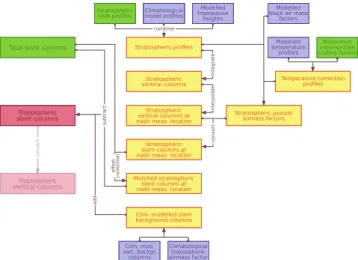
Fig. 1.Data flow of calculating tropospheric NO2 columns from
SCIAMACHY measurements. Measured and modelled quantities are shown in green and purple, respectively, while intermediate re-sults are marked in yellow. Conversion of SCDtropto VCDtrop
in-volves calculation of tropospheric air mass factors, the discussion of which is beyond the scope of this study.
to relatively low global coverage, making the derivation of global fields from these measurements a challenging task.
In this study, we calculate one stratospheric NO2column for every single SCIAMACHY nadir measurement. Whilst having the disadvantage of not attaining global coverage with the resulting stratospheric data product, this has the advan-tage of avoiding the need to average over several days of measurements, as, for example, in Beirle et al. (2010). The interpolated VCDstrat are then converted to slant columns using stratospheric air mass factors (Sect. 3.3). Following this step, the limb stratospheric slant columns are adjusted to the level of the SCDtot from nadir measurements using an additive offset (Sect. 3.4), taking into account the tropo-spheric contribution to the measured signal (Sect. 3.5). The full procedure is depicted in Fig. 1.
3.1 Calculating stratospheric NO2columns
Based on the measured and modelled number concentration profilesnlimb(t, h, ϕ, ψ )[molec cm−3] and nmod(t, h, ϕ, ψ ) [molec cm−3], respectively, and on the tropopause heights
htrop(t, ϕ, ψ )[m], stratospheric NO2 profiles are calculated for timet, latitudeϕ, and longitudeψas follows: The mod-elled NO2 profiles are compiled into a monthly climatol-ogynmod(m(t ), h, ϕ, ψ ). Lethlimb
the combined stratospheric profile as
nlimbstrat(t, h, ϕ, ψ )=
0 ifh < htrop(t, ϕ, ψ )
nmod(m(t ), h, ϕ, ψ )ifhtrop(t, ϕ, ψ )≤h < hlimbmin(t, ϕ, ψ )
nlimb(t, h, ϕ, ψ ) ifh≥hlimbmin(t, ϕ, ψ ).
(1)
The combined limb/model number density profiles are then vertically integrated into stratospheric columns:
VCDlimbstrat(t, ϕ, ψ )=
TOA
Z
h=htrop(t,ϕ,ψ )
nlimbstrat(t, h, ϕ, ψ )dh. (2)
For the Oslo CTM2, vertical stratospheric columns VCDmodstrat(t, ϕ, ψ )are calculated accordingly.
3.2 Interpolation to nadir measurement location
Both the model and the limb stratospheric NO2column prod-ucts used in this study are only available on a horizontal res-olution that is much coarser than the spatial extents of in-dividual SCIAMACHY nadir measurements (usually 60× 30 km2). Therefore, we need to interpolate the coarse strato-spheric columns to the locations of each SCIAMACHY nadir measurement to ensure the best possible spatial matching.
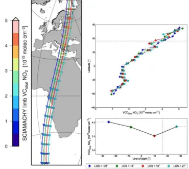
For SCIAMACHY limb measurements, several steps are required in order to calculate stratospheric NO2columns for each nadir measurement, processing each orbit separately. This procedure is illustrated in Fig. 2. First, we assign a fixed azimuth angle to each of the four discrete limb line-of-sight directions, namely−25◦, −8◦, 10◦ and 27◦. These angles are chosen to be the mean viewing azimuth angles of those nadir pixels which fall into the field of view of the respective limb state.1
Next, we consider the stratospheric NO2 column den-sity along each line-of-sight as depending only on latitude. For each nadir pixel at timet, latitudeϕ, and longitudeψ, we calculate four stratospheric columns VCDistrat(t, ϕ, ψ )by linearly interpolating along-track, that is along each view-ing directioni. For both limb and nadir measurements, we only take into account the descending parts of the orbit to avoid complications from measurements taken at different local times and therefore photochemical states. Finally, for all nadir pixels, we consider the stratospheric NO2column to be a function of the line-of-sight, and linearly interpolate the correct column density from the four column densities previously calculated.
In the case of Oslo CTM2 simulations, the modelled NO2 columns are interpolated to the location and time of the in-dividual nadir measurements using smoothing cubic splines and linear interpolation, respectively.
1In this case a negative angle describes a point west of the nadir
point, while a positive angle describes a location east of the nadir point.
Fig. 2. Interpolation of stratospheric NO2 columns from
SCIAMACHY limb measurements to the location of the same or-bit’s nadir measurements. As an example, we calculate VCDstratfor
the nadir measurement located at 54.25◦N/32.25◦E from
SCIA-MACHY orbit no. 32984 (21 June 2008). In a first step, each limb state is treated independently. For each state, VCDstratis considered
to be a function of latitude only (left). To calculate a VCDstratvalue
for one single nadir measurement, at first, one VCDstratper state
is calculated by linear interpolation in latitude (top right). Finally, the VCDstratvalue corresponding to the nadir measurement of
in-terest is calculated by linear interpolation in the line-of-sight angle (bottom right).
For ease of notation, we will call the interpolated NO2 columns again VCDlimbstrat(t, ϕ, ψ ) and VCDmodstrat(t, ϕ, ψ ) for SCIAMACHY limb and Oslo CTM2, respectively.
Monthly averages of VCDlimbstrat(t, ϕ, ψ ), gridded to 0.125◦, are shown in Fig. 3.
3.3 Stratospheric air mass factor (AMF)
We use the radiative transfer model SCIATRAN (Rozanov et al., 2005b) to calculate a lookup table of block air mass factors (BAMF) for 31 solar zenith anglesϑ(SZA) between 10◦and 92◦, and for 101 uniformly spaced altitude layersh from sea level (0 km) to 100 km.
0 1 2 3 4 5
VCDstrat NO2 [1015 molec cm−2]
Fig. 3.Monthly averages of VCDlimbstrat NO2from SCIAMACHY
limb measurements for June 2010, interpolated to the locations of the SCIAMACHY nadir measurements, and binned to 0.125◦.
overestimation of the stratospheric NO2 column. This will subsequently be corrected for by an increased air mass fac-tor.2 To these means, we introduce the correction function
ftcorr(T ), based on the idea presented in Boersma et al. (2004):
ftcorr(T )=
3.826×10⁻³
×T +0.1372 3.826×10⁻³×T
0+0.1372
. (3)
This correction function has been derived by comparing dif-ferential cross sections measured at four distinct tempera-tures between 221 K and 293 K and is described by N¨uß et al. (2006).T0is the temperature at which the cross section used in the fit has been measured; in our case,T0=243 K. The
stratospheric air mass factor at timet, latitudeϕ, longitude
ψ, SZAϑand viewing zenith angleαis then calculated as
AMFlimbstrat=
1
cosα−1
+
TOA
Z
h=htrop
BAMF×nlimbstrat
ftcorr(T )×VCDlimbstrat dh, (4)
and accordingly AMFmodstratfor Oslo CTM2.
Temporal and spatial interpolation is done as described in Sect. 3.2, while the SZA interpolation is linear.
3.4 Offset limb/nadir
The stratospheric vertical columns derived from SCIA-MACHY limb measurements and Oslo CTM2 simulations differ considerably from total vertical columns obtained over the clean Pacific region from SCIAMACHY nadir measure-ments by applying a stratospheric air mass factor, which we call VCDnadirstrat3. In this study, we will use the Pacific region 2To be precise, one should speak of pseudo air mass factors
when they incorporate the temperature correction.
3VCDnadir
strat still contains the tropospheric contribution to the
measured signal.
180 120 60 0 60 120 180
Longitude [°]
2.8 3.0 3.2 3.4 3.6 3.8
VC
Dstrat NO2
[10
15mo
lec
cm
2] Aug 2006 60 N 65 N
SCIA limb Oslo CTM2 SCIA nadir
Fig. 4.Zonal variation of VCDlimbstratfrom SCIAMACHY limb
mea-surements (red), VCDmodstratfrom Oslo CTM2 simulations (blue), and of VCDnadirstrat from SCIAMACHY nadir measurements. Monthly mean values for August 2006, between 60◦and 65◦N.
between longitudes 180◦W and 150◦W to correct for this ef-fect. This region will subsequently be called “reference sec-tor”. An example of the latitude- and time-dependent offset is shown in Fig. 4 for northern latitudes in August 2006.
In order to account for these systematic biases, we apply a daily, latitude-dependent offset to all limb and modelled stratospheric columns to force them to the base level of the nadir measurements.
3.5 Pacific background
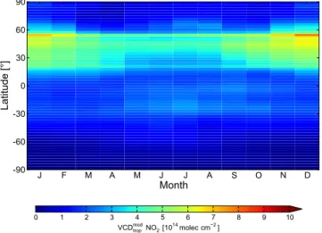
Before the stratospheric columns from SCIAMACHY and Oslo CTM2 can be adjusted to the level of the total nadir columns over the Pacific, the latter must be corrected for pos-sible tropospheric NO2signals. As independent, appropriate measurements over the Pacific Ocean are extremely sparse, we use climatological NO2data derived from the same run of the Oslo CTM2 model as used for the stratospheric columns (see Sect. 2.4). The data show that the tropospheric NO2 content over the Pacific Ocean is negligibly small most of the time. Only in northern mid-latitudes, and there especially during winter, significant amounts of tropospheric NO2are predicted by the model (see Fig. 5).
These enhanced NO2 columns can most probably be at-tributed to exported pollution from Eastern Asia and North America, as the lifetime of tropospheric NO2is strongly en-hanced during winter.
Similar corrections have been previously performed by Martin et al. (2002).
From the modelled NO2 fields nmod(t, h, ϕ, ψ ) [molec cm−3], we calculate vertical tropospheric columns over the reference sector as
VCDmodtrop(t, ϕ, ψ )=
htrop(t,ϕ,ψ ) Z
h=0
nmod(t, h, ϕ, ψ )dh. (5)
J F M A M J J A S O N D
Month
-90 -60 -30 0 30 60 90
Latitude [°]
0 1 2 3 4 5 6 7 8 9 10
VCDmod
tropNO2[1014molec cm2]
Fig. 5. Climatology of VCRmodtrop NO2 over the Pacific Ocean
(180◦W–150◦W) for the years 1998–2007, computed from Oslo
CTM2 simulations.
As tropospheric air mass factors, we use the dataset de-veloped by N¨uß (2005), which was derived using the ra-diative transfer model SCIATRAN (Rozanov et al., 2005b) and NO2 profiles from the MOZART4 model. We compile a monthly climatology of air mass factors over the refer-ence sector AMFRtrop(m, ϕ)by zonally averaging over the AMFtropfor all SCIAMACHY nadir measurements in month
mand at latitudeϕover the reference sector during the 2003– 2011 time period.
The monthly climatology of modelled tropospheric back-ground columns is then converted to slant columns via SCRmodtrop(m, ϕ)=VCRmodtrop(m, ϕ)×AMFRtrop(m, ϕ). (6)
3.6 Applying stratospheric correction
We calculate the stratospheric slant columns on a daily ba-sis. The limb, nadir, and modelled datasets are compiled into zonally averaged daily aggregates over the reference sector, yielding SCRlimbstrat(t, ϕ), SCRnadirstrat(t, ϕ), and SCRmodstrat(t, ϕ), re-spectively. These daily averages are then linearly interpo-lated in latitude, and smoothed temporally, to account for days and latitudes with missing measurements over the Pa-cific Ocean. We call the resulting quantities SCRlimbstrat(d, ϕ), SCRnadirstrat(d, ϕ), and SCRmodstrat(d, ϕ).
The desired stratospheric slant columns are then calculated by applying the additive offset, derived from the averaged limb (or model) and nadir columns over the reference sector, and forcing the resulting tropospheric slant columns to equal the modelled background columns SCRmodtrop(m, ϕ):
SCDlimbstrat =VCDlimbstrat×AMFlimbstrat+
SCRnadirtot −SCRlimbstrat−SCRmodtrop (7) and accordingly SCDmodstratfor Oslo CTM2.
0.0 0.5 1.0 1.5 2.0 2.5 3.0
NO2 concentration [109molec. cm3] 0
10 20 30 40 50
Altitude [km]
0.0 0.5 1.0 1.5 2.0 2.5 3.0 3.5
NO2 concentration [109molec. cm3] 0
10 20 30 40 50
Altitude [km]
0 1 2 3 4 5
NO2 concentration [109molec. cm3] 0
10 20 30 40 50
Altitude [km]
0.0 0.5 1.0 1.5 2.0 2.5 3.0
NO2 concentration [109molec. cm3] 0
10 20 30 40 50
Altitude [km]
SCIAMACHY limb
Limb climatology Oslo CTM2Mod. climatology Combined datasetU.S. std. atm. 1976
Fig. 6. Vertical NO2 profiles from SCIAMACHY limb (actual
measurement: red, climatology: magenta), Oslo CTM2 (actual value: blue, climatology: cyan), and US Standard Atmosphere 1976 (green) for 1 June 2007, at 3.48◦W, 58.66◦N (top left); 2 July 2007,
at 58.54◦W, 63.7◦N (top right); 18 February 2007, at 70.54◦W,
75.50◦S (bottom left); and 27 March 2006, at 5.17◦E, 40.65◦N
(bottom right). The tropopause altitude is shown as a black dashed line, while the combined limb measurements/model climatology profile used for the column and air mass factor calculations in this study are marked as black stars.
These SCDlimbstrat/mod(t, ϕ, ψ ) are the final output of our stratospheric correction algorithm. They can be directly sub-tracted from retrieved nadir total slant columns to yield tropospheric slant columns.
4 Results and discussion
4.1 Stratospheric NO2from SCIAMACHY limb and
Oslo CTM2
4.1.1 Vertical profiles
As described in Sect. 3.1, we extend the SCIAMACHY limb profiles down to the tropopause, using climatological profiles from the Oslo CTM2 simulations for the years 1998–2007. Figure 6 illustrates that this approach is valid: the profiles measured by SCIAMACHY are similar enough to the clima-tology of those modelled by Oslo CTM2, especially in the altitude regions between the tropopause and 11 km, where NO2concentrations are relatively small.
J F M A M J J A S O N D
Month
-90 -60
-300
30 60 90
VCDstrat((Nadir BG) Limb)
J F M A M J J A S O N D
-90 -60
-300
30 60 90
VCDstrat(Nadir Limb)
J F M A M J J A S O N D
-90 -60
-300
30 60 90
Latitude [°]
SCDstrat(Nadir Limb)
J F M A M J J A S O N D
Month
-90 -60
-300
30 60 90
Latitude [°]
SCDstrat((Nadir BG) Limb)
12 10 8 6 4 2 0 2
[1014molec cm2]
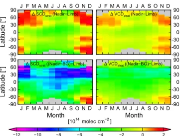
Fig. 7. Monthly climatology of the difference between
SCIA-MACHY nadir and limb measurements over the Pacific Ocean (180◦W–150◦W), averaged from the years 2004–2010 and
grid-ded into 2.5◦latitude bins.1VCDstrat(left) and1SCDstrat(right),
“raw” columns (top) and after subtracting the tropospheric influence from the Oslo CTM2 climatology (bottom).
to the SCIAMACHY instrument due to vertical smooth-ing. At that time of year (early July) and in those latitude regions (65◦N), the ECMWF-IFS temperature fields show a layer of enhanced temperature around 14 km. This could drive the decomposition of N2O5and HO2NO2, two species which are especially sensitive to temperature changes, lead-ing to increased NO2concentrations. Since this feature can be observed at all longitudes, the increased temperature and NO2 are unlikely to be caused by terrain effects. In these situations, the stratospheric columns resulting from SCIA-MACHY observations will be a few percent smaller than those from the model.
4.1.2 Difference to nadir measurements
As described in Sect. 3.4, the NO2 columns retrieved from SCIAMACHY nadir and limb measurements show a system-atic offset. This offset has already been observed previously (Beirle et al., 2010). Figure 7 (top) shows the magnitude of this offset over the Pacific Ocean (180◦W–150◦W). It ranges from+3×10¹⁴molec cm−2in near-polar latitudes in Decem-ber to−4×10¹⁴molec cm−2in polar latitudes in austral win-ter. In the tropics and mid-latitudes, the offset varies between
−1×10¹⁴ and−3×10¹⁴molec cm−2, with a minimum in June/July. The same annual cycle can be observed in all lati-tude bands, with minima in June and July, and maxima in De-cember and January. In the months October to March, outside the tropics, nadir columns can be larger than limb columns by about 5–6×10¹⁴molec cm−2in individual months.
However, the measured nadir columns still contain a tro-pospheric contribution. After subtracting this modelled back-ground signal (see Sect. 3.5), the stratospheric NO2 from
limb measurements is higher than from nadir geometry al-most globally. Only in austral summer, nadir measurements show larger NO2 values than limb (Fig. 7, bottom). This could point to possible issues in the nadir retrieval from SCIAMACHY measurements, as Richter et al. (2011) re-ported that over clean background regions, vertical NO2 columns from SCIAMACHY are smaller than those from GOME-2 by 2–3×10¹⁴molec cm−2– too much to be solely explained by diurnal differences caused by the local mea-surement time. Another possible explanation might lie in the different wavelength windows used for the retrievals (425–450 nm vs. 420–470 nm for nadir and limb, respec-tively); however, this seems unlikely to be the only cause.
The offset shows both a clear seasonal cycle and strong meridional variation. The seasonal variation suggests that in regions where frontal systems are modulating the tropopause height, we might be observing a varying systematic differ-ence between limb and nadir measurements. The latitudi-nal variability of the offset looks very similar to that of the modelled background climatology, suggesting that the Oslo CTM2 overestimates the lifetime of tropospheric NO2, especially in winter.
While generally the observed differences are small in ab-solute numbers and are well within the expected uncertainties of the two measurements, they do have a significant effect on the retrieved tropospheric columns and therefore need to be corrected for. Overall, further work is needed to investigate this phenomenon in more detail. In the study of tropospheric NO2, which is dominated by lower atmospheric sources and chemical removal of NOx, the taken approach for empirically removing its effect is however appropriate.
4.1.3 Climatological comparison measurement/model
To compare measured and modelled stratospheric NO2 columns, we calculate their correlation for the five years 2003–2007 for which both measurements and model results are available. Figure 8 shows a scatter plot of the monthly mean values of the VCDstratNO2between 60◦S and 60◦N, interpolated to the locations (and, for the model data, times) of the nadir measurements, and gridded to a 0.125◦ grid. The Pearson correlation coefficient of the two grid-ded datasets is 0.974, showing excellent correlation. How-ever, the Oslo CTM2 consistently overestimates the mea-sured NO2 columns, which can be seen from the slope of 0.94. When all latitudes are considered, the correlation coef-ficient almost remains unchanged, while the slope of the cor-relation line decreases to 0.88, showing systematically larger stratospheric NO2columns from the model at high latitudes. From the comparison of the measured and modelled vertical profiles, it becomes apparent that the systematic overestima-tion is mostly coming from altitudes lower than 30 km (see Sect. 4.1.1).
Fig. 8.Scatter plot of monthly mean values for VCDstratNO2from
SCIAMACHY limb measurements and Oslo CTM2 simulations for the 2003–2007 time period, for the latitudes between 60◦S and
60◦N. The red line marks the linear regression fit (slope 0.94, offset −3.3×10¹³). The Pearson correlation coefficient of the two datasets is 0.974.
remarkably well, after removing an offset between the two datasets. Figure 9 shows the average difference between the two datasets for the 2003–2007 period and for three selected climatological monthly means.4 The difference of the five-year averages has been offset so that it amounts to 0 over the reference sector (180◦W–150◦W). Systematic differences in the vertical columns are smaller than 5×10¹³molec cm−2. The spatial pattern of these differences is interesting, show-ing a clear seasonality and, in some regions, e.g. the South American west coast, a strong land–sea contrast. One possi-ble explanation might be an orographic effect stemming from the comparably low resolution of the Oslo CTM2. Another possible source for the observed spatial patterns might be the model’s treatment of clouds and their influence on pho-tochemistry; however, the photochemistry is mostly deter-mined by the short wavelengths, which usually do not pene-trate deep enough to be affected by clouds, especially at high latitudes.
The possible influence of clouds has been investigated by filtering for scenes with less than 20 % cloud cover from the FRESCO+ dataset (version 6, Wang et al., 2008). In
gen-4See Supplement for plots of the months not shown in Fig. 9.
July
−4 −3 −2 −1 0 1 2 3 4
∆VCDstrat NO2 [1014 molec cm−2]
annual mean February
October
Fig. 9. The difference 1VCDstrat NO2 between SCIAMACHY
limb and Oslo CTM2 for the 2003–2007 time period. Red and blue areas correspond to regions where SCIAMACHY limb measure-ments are larger and smaller than Oslo CTM2 simulations, respec-tively. Top left: average difference over all months. Top right: av-erage difference of all Februaries. Bottom left: avav-erage difference of all Julies. Bottom right: average difference of all Octobers. An additive offset has been applied to force the difference to equal zero over the reference sector (180◦W–150◦W).
eral, our findings show that clouds cannot be made respon-sible for the observed spatial patterns. The only exceptions are the Antarctic coast, where the cloud-screened data lack the large area of positive differences seen in the full dataset, and the Canadian Hudson Bay area, where the difference in the cloud-screened data turns negative from the positive val-ues in the full dataset. In the case of the Antarctic coast, the large positive differences come mostly from austral spring (September and October). Both effects can, most probably, be attributed to the FRESCO+ cloud algorithm having dif-ficulties in identifying clouds over bright surfaces, which in turn leads to an under-representation of winter values in the climatological average.
The impact of clouds should be explored further, cause the understanding of the systematic differences be-tween limb retrievals and model simulations might improve our knowledge of the influence of clouds and surface spectral reflectance on atmospheric photochemistry.
4.1.4 Zonal variability of stratospheric NO2columns
180 120 60 0 60 120 180
Longitude [°]
2.4 2.6 2.8 3.0 3.2
VC
Dstrat NO2
[10
15mo
lec
cm
2] Aug 2006 60 N 65 N
180 120 60 0 60 120 180
Longitude [°]
3.0 3.1 3.2 3.3 3.4 3.5 3.6 3.7
VC
Dstrat NO2
[10
15mo
lec
cm
2] Aug 2006 70 N 75 N
SCIA limb Oslo CTM2 SCIA nadir ref. sect.
Fig. 10.Zonal variation of VCD′limb
strat, VCD′stratmod, and VCD′stratnadir.
The nadir measurements’ value over the reference sector is marked as dashed black line. Monthly mean values for August 2006, be-tween 60◦and 65◦N (top) and between 70◦and 75◦N (bottom).
from the offset-corrected SCDlimbstratand SCDmodstratvia VCD′limb
strat =
SCDlimbstrat
AMFlimbstrat (8)
VCD′mod strat =
SCDmodstrat
AMFmodstrat. (9)
For comparison, we show the “stratospheric” vertical column derived from SCIAMACHY nadir measurements as
VCD′nadir strat =
SCDnadirtot −SCRmodtrop
AMFlimbstrat . (10)
First, it is noticeable that the zonal variability of SCIA-MACHY limb measurements and Oslo CTM2 simulations is remarkably similar (see Fig. 10, top). However, the simulated stratospheric columns are often larger than the measured val-ues, which is also shown by the linear regression of the two datasets (cf. Fig. 8). The two stratospheric datasets agree rea-sonably well with the nadir measurements in unpolluted re-gions (see Fig. 10, top).
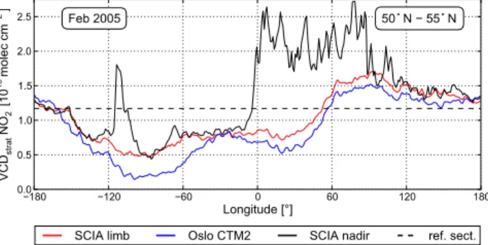
One noticeable feature in all datasets is a systematic low in the observed VCDstratNO2over Greenland (∼50◦W) in
summer (June–September), a pattern which can be seen in all years 2003–2011 (see Fig. 10 for August 2006). Since this feature is present in both datasets and persistent over the years, we deem it unlikely to be a retrieval or mod-elling artifact. The area of southern Greenland is known to be special for multiple reasons. There exists strong tropopause
180 120 60 0 60 120 180
Longitude [°]
0.0 0.5 1.0 1.5 2.0 2.5
VC
Dstrat NO2
[10
15mo
lec
cm
2] Feb 2005 50 N 55 N
SCIA limb Oslo CTM2 SCIA nadir ref. sect.
Fig. 11.Zonal variation of VCD′limb
strat, VCD′stratmod, and VCD′stratnadir.
The nadir measurements’ value over the reference sector is marked as dashed black line. Monthly mean values for February 2005, be-tween 50◦and 55◦N.
folding activity (Elbern et al., 1998) and thus troposphere-stratosphere exchange (Sprenger and Wernli, 2003). Further-more, a local maximum in the density of polar low pressure systems exists to its east (see Zahn and von Storch, 2008), and Greenland’s high surface altitude and high surface re-flectance (due to ice cover) stand in clear contrast to the sur-rounding Atlantic Ocean. While all these factors might con-tribute to the observed summer lows in VCDstrat NO2, the underlying mechanisms remain unclear at the moment, and it is difficult to clearly attribute this phenomenon to one of them.
While generally the shape of the zonal variation is very similar between SCIAMACHY limb and Oslo CTM2, in some cases, the amplitudes can differ significantly. An ex-ample is shown in Fig. 11, where, after applying the off-set, the agreement between nadir and limb measurements is mostly excellent in those regions without tropospheric pol-lution. The simulated VCD′mod
strat, however, are slightly lower than the measured ones, indicating that the model might be overestimating the stratospheric NO2over the Pacific Ocean, leading to an exaggerated bias correction.
180 120 60 0 60 120 180
Longitude [°]
0.0 0.2 0.4 0.6 0.8 1.0 1.2 1.4
VC
Dstrat NO2
[10
15mo
lec
cm
2] Dec 2004 50 N 55 N
SCIA limb Oslo CTM2 SCIA nadir ref. sect.
Fig. 12.Zonal variation of VCD′limb
strat, VCD′stratmod, and VCD′stratnadir.
The nadir measurements’ value over the reference sector is marked as dashed black line. Monthly mean values for December 2004, be-tween 50◦and 55◦N.
NO2 burden over North America when using the modelled NO2fields for stratospheric correction.
In cases like this, the assessment of tropospheric pollution can be severely influenced by the used stratospheric correc-tion, especially over North America. Figure 12 shows another example (January 2005, 50◦–55◦N), when using the refer-ence sector method, only the pollution signals of the cities Montr´eal, Toronto and Edmonton would be visible as posi-tive tropospheric columns, but the actual VCDtropwould be underestimated by more than 50 %. This is again caused by the fact that the Pacific Ocean stratosphere often contains larger NO2columns than the zonally adjacent areas.
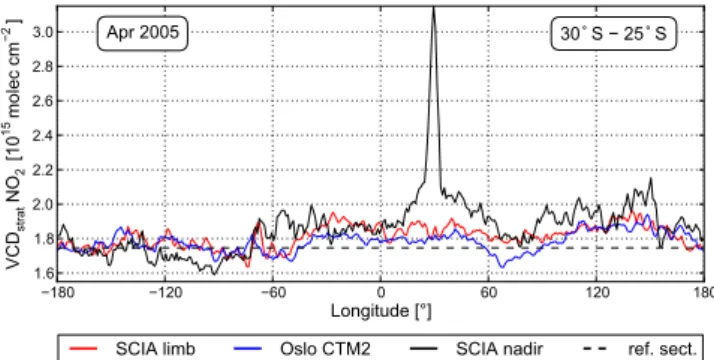
Finally, an interesting issue regarding the nadir ments can be identified by comparing them to limb measure-ments. In many months, the retrieved nadir columns seem to be lower than the integrated limb stratospheric measure-ments off the Chilean coast in the East Pacific (∼75–80◦W). As it can be seen in Fig. 13, the VCD′nadir
strat from nadir mea-surements are lower than those from limb meamea-surements and model simulations by about 1×10¹⁴molec cm−2. In this case, it seems not to be an artefact originating from the ref-erence sector offset, as the nadir measurements are signifi-cantly higher than the limb measurements at many other lon-gitudes. This might be a hint leading to issues in the nadir retrieval over clean ocean waters, for example from liquid water absorption or vibrational Raman scattering in water (Vountas et al., 2003; Lerot et al., 2010). A more system-atic investigation of this is needed, but outside the scope of this study.
4.1.5 Comparison of the day-to-day variability
Particular attention needs to be paid to the variability of the different stratospheric datasets. The very sparse spatial cov-erage of the limb measurements could lead to large variabil-ity of the interpolated data product. As this would severely interfere with its usability for stratospheric correction, we in-vestigate this issue by comparing the variability of the
strato-180 120 60 0 60 120 180
Longitude [°]
1.6 1.8 2.0 2.2 2.4 2.6 2.8 3.0
VC
Dstrat NO2
[10
15mo
lec
cm
2] Apr 2005 30 S 25 S
SCIA limb Oslo CTM2 SCIA nadir ref. sect.
Fig. 13.Zonal variation of VCD′limb
strat , VCD′stratmod, and VCD′stratnadir.
The nadir measurements’ value over the reference sector is marked as dashed black line. Monthly mean values for April 2005, between 30◦and 25◦S.
spheric vertical columns. For 2005, we calculated daily av-erages of all data points (measurement pixel centres/model grid cell centres) within 5.6◦×5.6◦ boxes, located at 180◦ longitude and nine different latitudes. Figure 14 shows the daily time series. Both limb measurements and modelled columns are taken from the “raw” datasets, i.e. neither spa-tial interpolation nor offset correction have been applied. Oslo CTM2 values in high latitude winter are unrepresenta-tive since at SCIAMACHY measurement time (to which the modelled data have been interpolated), the sun is still below the horizon, and the model state therefore represents night-time chemistry.
SCIAMACHY limb measurements generally yield higher VCDstrat NO2 than Oslo CTM2 simulations and SCIAMACHY nadir measurements, at low and mid-latitudes. At very low solar zenith angles, however, Oslo CTM2 simulations show considerably higher NO2 values, especially in the Southern Hemisphere. This is most proba-bly due to the difficult determination of the average overpass time of one model grid cell at such high latitudes, which might cause significant errors when the overpass time can vary considerably within one model grid cell.
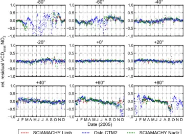
As a measure to compare the variabilities of the three datasets, we compute the coefficients of variationcv.
We calculate daily residuals by subtracting a centred 31-day moving average from the daily time series (see Fig. 15), and definecvas the ratio of their standard devia-tion and sample mean (see Table 1).
0.0 1.0 2.0 3.0 4.0 5.0 6.0 -75° 0.01.0 2.0 3.0 4.0 5.0 6.0 -58° 0.0 1.0 2.0 3.0 4.0 5.0 6.0 -39° 0.0 1.0 2.0 3.0 4.0 5.0 6.0 VC
Dstrat NO2 [10 15mo lec cm 2] -20° 0.01.0 2.0 3.0 4.0 5.0 6.0 +0° 0.0 1.0 2.0 3.0 4.0 5.0 6.0 +20°
J F M A M J J A S O N D 0.0 1.0 2.0 3.0 4.0 5.0 6.0 +39°
J F M A M J J A S O N D
Date (2005) 0.01.0 2.0 3.0 4.0 5.0 6.0 +58°
SCIAMACHY Limb Oslo CTM2 SCIAMACHY Nadir
J F M A M J J A S O N D 0.0 1.0 2.0 3.0 4.0 5.0 6.0 +75°
Fig. 14.Daily time series for the year 2005 of VCDstratNO2from
SCIAMACHY limb (red), Oslo CTM2 (blue), and of VCDtotfrom
SCIAMACHY nadir (stratospheric air mass factor applied, green) for nine 5.6◦×5.6◦grid boxes. The centres of the grid boxes are
located at 180◦longitude and the latitudes are given in the plot titles.
in the nadir retrieval as compared to the limb retrieval. We conclude that the measurement noise in the individual limb columns, while being significant, does not severely impact the retrieval of tropospheric NO2columns.
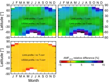
4.2 Sensitivity study: impact of air mass factor
calculations
As described in Sect. 3.3, the integrated and interpolated VCDstratneed to be converted to slant columns. The simplest approach is to use an air mass factor based on a single atmo-spheric profile, e.g. the climatological stratoatmo-spheric NO2 pro-file from the US Standard Atmosphere 1976 (Committee on Extension to the Standard Atmosphere, 1976), and to assume a constant surface reflectivity, e.g. 0.05. The influence of the surface reflectivity on the stratospheric AMF is reported to be very low (Wenig et al., 2004), which is why this effect is not further investigated within this study. Figure 16 (bot-tom left) shows the relative change of the stratospheric AMF introduced by using the actual stratospheric NO2 profile as measured by SCIAMACHY. In virtually all cases, the influ-ence of the assumed NO2profile on the stratospheric air mass factors is negligible. Only in polar latitudes in winter does as-suming the stratospheric NO2profile from the US Standard Atmosphere lead to an overestimation of stratospheric AMFs by up to 4.5 %.
To assess the influence of the temperature dependence of the NO2 absorption cross section on the stratospheric NO2 correction (see Sect. 3.3), we performed a sensitivity study on eight years of data from 2003 until 2010. We used the same ECMWF forecast temperature profiles which were used in the limb retrieval. Our results show that the
temper-1.0 0.5 0.0 0.5 1.0 -80° 1.0 0.5 0.0 0.5 1.0 -60° 1.0 0.5 0.0 0.5 1.0 -40° 1.0 0.5 0.0 0.5 1.0 rel. re sid ua l V CDstr at
NO2 -20°
1.0 0.5 0.0 0.5 1.0 +0° 1.0 0.5 0.0 0.5 1.0 +20°
J F M A M J J A S O N D 1.0
0.5 0.0 0.5
1.0 +40°
J F M A M J J A S O N D
Date (2005) 1.0 0.5 0.0 0.5 1.0 +60°
SCIAMACHY Limb Oslo CTM2 SCIAMACHY Nadir
J F M A M J J A S O N D 1.0
0.5 0.0 0.5
1.0 +80°
Fig. 15.Time series for the year 2005 of the relative residuals of
VCDstratNO2from SCIAMACHY limb (red), Oslo CTM2 (blue),
and of VCDtot from SCIAMACHY nadir (stratospheric air mass
factor applied; green) for nine 5.6◦×5.6◦grid boxes. The centres
of the grid boxes are located at 180◦ longitude and the latitudes
are given in the plot titles. The residuals have been computed by subtracting a centred 31-day moving average from the daily dataset.
Table 1.Coefficients of variationcv=µσ (σbeing the standard
de-viation, andµbeing the sample mean) of daily VCDstratNO2for
nine 5.6◦×5.6◦grid boxes located at 180◦longitude for the year
2005.
Latitude SCIA limb SCIA nadir Oslo CTM2
−80◦ 0.199 0.359 0.603 −60◦ 0.328 0.435 0.325 −40◦ 0.236 0.313 0.233 −20◦ 0.133 0.205 0.129
0◦ 0.088 0.091 0.035
20◦ 0.111 0.156 0.161
40◦ 0.147 0.226 0.218
60◦ 0.302 0.370 0.448
80◦ 0.265 0.298 0.419
ature dependence of the NO2absorption cross section actu-ally has significant influence on stratospheric air mass fac-tors. As it can be seen in Fig. 16 (top right), the temperature dependence influences the stratospheric air mass factors by between 5 % and 15 %; using a fixed temperature of 243 K leads to an underestimation of the AMF. The influence is highest for the winter months and can reach up to 15 % at polar latitudes in the climatological mean.
J F M A M J J A S O N D
-90 -60
-300
30 60 90
Latitude [°]
Limb-profile / T-corr -USStd-profile / no T-corr
J F M A M J J A S O N D
-90 -60
-300
30 60 90
Limb-profile / T-corr -Limb-profile / no T-corr
J F M A M J J A S O N D
Month
-90 -60
-300
30 60 90
Latitude [°]
Limb-profile / no T-corr -USStd-profile / no T-corr
5 0 5 10 15
AMFstrat relative difference [%]
Fig. 16.Monthly climatologies of the influence of stratospheric
NO2profiles and temperature correction on stratospheric air mass
factors. The plots show the influence of both profiles and temper-ature correction (top left), tempertemper-ature correction alone (top right), and vertical profiles alone (bottom left). The climatologies are cal-culated for the years 2003–2010, using all retrieved limb profiles from the descending part of the SCIAMACHY orbit. The influ-ence of the vertical profile is derived by comparing to using the US Standard Atmosphere’s NO2profile. Stratospheric temperature
pro-files are taken from the ECMWF forecast (the same propro-files used in the limb retrieval). The geometric line-of-sight correction (the sum-mandcos1α−1) has been ignored in this comparison, and the relative difference of two datasets is computed as a−b
(a+b)/2.
show that the simple AMF underestimates the accurate one by ca. 2–14 % (Fig. 16, top left).
4.3 Improvements to the tropospheric data product
When using SCIAMACHY limb measurements or Oslo CTM2 simulations as a stratospheric correction scheme in-stead of the reference sector method, the data quality of the resulting fields of tropospheric slant columns improves considerably. Figure 17 shows SCDtrop NO2 for February 2005, using the reference sector method, SCIAMACHY limb measurements, and Oslo CTM2 simulations as stratospheric correction schemes. Compared to using the reference sec-tor method, both of the other stratospheric corrections con-siderably reduce the number of negative tropospheric NO2 columns.
The SCDlimbtrop for a single day (28 January 2006) are shown in Fig. 18.5 Compared to the data shown by Beirle et al. (2010), our results appear to be slightly less noisy. This might be because our approach accounts for possible small-scale variability in stratospheric NO2abundances. The most strik-5Additional days are shown in the Supplement. All days have
been chosen to allow easy comparison to the results of Beirle et al. (2010).
Fig. 17. Monthly average of SCDtrop NO2 from SCIAMACHY
for February 2005, using the reference sector method (top), SCIAMACHY limb measurements (centre), and Oslo CTM sim-ulations (bottom) as stratospheric correction.
ing difference, however, is the almost complete lack of sig-nificantly negative tropospheric NO2 columns in our data product. This is mostly due to the fact that we account for the NO2content of the Pacific troposphere, contrary to the “relative limb correction” of Beirle et al. (2010).
28 Jan 2006
−5 −4 −3 −2 −1 0 1 2 3 4 5 SCDtrop NO2 [1015 molec cm−2]
Fig. 18.SCDtrop NO2from SCIAMACHY for 28 January 2006,
using SCIAMACHY limb measurements as stratospheric correction schemes.
Scandinavia region shows a very clear seasonal cycle, with large negative values in winter. While the large amplitude of the oscillations is mostly due to the varying measurement geometry, the fact that the monthly mean values are consis-tently negative results from the observation already made in Sect. 4.1.4, where we showed that, especially in polar win-ter, stratospheric NO2fields are far from being zonally ho-mogeneous. Most often, stratospheric NO2 between 60◦N and 75◦N seems to peak over the reference sector – a result which is backed by investigation of the zonal variability of the stratospheric NO2 products (see Sect. 4.1.4). When us-ing SCIAMACHY limb measurements or Oslo CTM2 sim-ulations for stratospheric correction, these issues appear to be solved. The retrieved slant columns show a clear sea-sonal cycle with large winter maxima, as is to be expected from measurement geometry and enhanced lifetime of tro-pospheric NO2in winter due to photochemistry. The curves for SCIAMACHY limb and Oslo CTM2 qualitatively agree very well throughout the year, and during summer months, also with the reference sector method.
In the southern Atlantic region, results are similar. The large amplitudes of the reference sector time series in spring are gone when using limb measurements or Oslo CTM2 simulations for stratospheric correction. However, the SCIAMACHY and Oslo CTM2 datasets do not seem to agree as well. This might be due to the fact that the overall magnitude of the tropospheric slant columns is considerably smaller in this region, leading to a higher relative influence of the uncertainty in the stratospheric columns on the time series.
In the western Pacific region, a clear seasonal cycle can be seen independently of the used stratospheric correction. Dur-ing the summer months, all three datasets agree very well. During winter, however, the tropospheric slant columns re-trieved using the reference sector method are considerably
2003 2004 2005 2006 2007 2008 2009 2010 2011
0.01.0 2.0 3.0 4.0
5.0 North America
Reference sector SCIAMACHY Limb Oslo CTM2
-4.0 -2.00.0 2.0 4.0 6.0
8.0 Northern Scandinavia
-1.0 -0.50.0 0.51.0
1.5 Southern Atlantic
0.51.0 1.5 2.0 2.5
SC
Dtrop NO2
[10
15mo
lec
cm
2]
Western Pacific
Fig. 19.Time series of monthly mean values of SCDtrop NO2for
the regions labelled above as Northern Scandinavia (60◦N–75◦N,
0◦–40◦E), Southern Atlantic (50◦S–30◦S, 45◦W–15◦E), Western
Pacific (25◦N–50◦N, 148◦E–178◦E), and North America (40◦N–
60◦N, 120◦W–90 ◦W). Three different stratospheric correction
schemes have been used: SCIAMACHY limb measurements (red), Oslo CTM2 simulations (blue, only until 2007), and the reference sector method (black).
larger than the other two datasets, by as much as 60 %. This interesting feature might hint towards higher stratospheric NO2 columns in this region compared to the reference sec-tor, which is directly neighbouring to the east. While this observation is supported by the plots of zonal variability in Sect. 4.1.4, the reason for this repeating pattern is unclear.
Over North America, finally, the reference sector method leads to a clear underestimation of tropospheric pollution levels in winter. When either SCIAMACHY limb measure-ments or Oslo CTM2 simulations are used for stratospheric correction, however, the seasonal cycle becomes a lot more pronounced. The tropospheric columns in winter more than double in many years, while the summer lows remain almost unchanged.
4.4 Error analysis
4.4.1 Errors in the nadir measurements
than limb measurements by approximately 1014molec cm−2. In total, the retrieval errors amount to approximately 4× 10¹⁴molec cm−2 for the retrieved slant columns, which is less than 5 % (Richter et al., 1998; Boersma et al., 2004; Wenig et al., 2004).
Additionally, the nadir columns are subject to errors in-troduced by air mass factor calculations. For tropospheric columns over polluted regions, this is the dominating error source, which has been discussed elsewhere (Boersma et al., 2004; Leit˜ao et al., 2010; Heckel et al., 2011). Here, only the uncertainties introduced into the stratospheric contribu-tion of the signal are of interest. The vertical NO2profiles (taken from the limb measurements) as well as the temper-atures from the ERA-Interim reanalysis both contribute to these errors, but are difficult to quantify. The sensitivities of the resulting air mass factors to changes in the vertical absorber profile and to the temperature profile are given in Fig. 16, showing that uncertainties in these two quantities do not contribute significantly to the total error in most cases.
4.4.2 Errors in the limb measurements
Random errors in the measured radiances and systematic er-rors due to inaccuracies in the used absorption cross sections can influence the limb retrieval as well as the nadir retrieval. Instrument pointing errors can impact on the vertical resolu-tion and posiresolu-tion of the measured profiles, and the retrieval sensitivity decreases at lower altitudes. These error sources are discussed in detail in Bauer et al. (2012) and Rozanov et al. (2005a), and are expected to add up to less than 15 % of the VCDstratin most cases.
In those cases when the tropopause layer lies below the lower boundary of the limb profiles at 11 km, we extend the measured limb profiles with climatological profiles derived from Oslo CTM2 simulations (see Sect. 2.2). Errors in the climatological modelled vertical profiles can thus contribute to the total error of the stratospheric columns. However, our comparison of modelled and measured profiles shows that this effect can generally be neglected, as NO2number con-centrations in the UT/LS region are very low (see Fig. 6).
One further uncertainty comes from the radiative transfer modelling. Air masses from far away can contribute to the limb signal reaching the satellite, and spatial gradients can further complicate the situation. This effect has been studied in great detail in Puk¨ıte et al. (2010). Depending on the tan-gent height, the errors introduced to the retrieved NO2 con-centrations can be as large as 20 %. Puk¨ıte et al. (2010) show that these errors can be avoided by using a tomographic 2-D approach in the radiative transfer calculations. It is however not applicable in an operational data product, as it only im-proves the profile retrieval in the case of reduced distance between the individual SCIAMACHY measurements (3.3◦) obtained in dedicated limb-only orbits. Based on the findings of Puk¨ıte et al. (2010), we estimate the upper boundary of the error on the retrieved stratospheric columns to be 30 %
in some rare extreme cases of low absolute values, while in most situations, the associated error should not exceed 10 % of the VCDstrat.
4.4.3 Errors in the resulting tropospheric slant columns
Uncertainties in the tropospheric slant columns derived by the limb/nadir matching approach are determined by the un-certainties in both the nadir and limb observations as well as the model background added over the Pacific Ocean. Our study suggests that the random error in the strato-spheric columns retrieved from limb measurements is of the same magnitude as the one for nadir measurements (see Ta-ble 1), leading to an increase of the random errors in the re-sulting tropospheric slant columns by a factor of approxi-mately√2. Assuming a 10 % random uncertainty in the limb columns, and maximum stratospheric slant columns of about 1×10¹⁶molec cm−2at latitudes below 60◦, errors of up to 1×10¹⁵molec cm−2can be introduced. Systematic errors are to a large extent removed by adjusting the limb columns over the reference sector, but longitude-dependent offsets between limb and nadir measurements might still exist. Also, it must be noted that in cases when the visibility of tropospheric NO2 is reduced by cloud coverage in the reference sector, the off-set correction might lead to an underestimation of the strato-spheric slant columns and thus yield too high tropostrato-spheric columns. The resulting uncertainty in the tropospheric slant columns is bounded by the NO2content of the Pacific tropo-sphere and thus on the order of 2–4×10¹⁴molec cm−2 in most regions and times; only in the Northern Hemisphere winter are considerable amounts of NO2 predicted by the Oslo CTM2 model, leading to possibly larger errors. How-ever, it must be noted that currently, accepting this uncer-tainty seems to be unavoidable. While excluding cloudy pix-els from the calculation of SCDnadirtot for determining the Pa-cific offset correction would avoid the systematic underesti-mation of stratospheric slant columns, the cloud filter would remove a large amount of all measurements over the Pacific, considerably increasing the influence of random errors and noise (which would cancel out to a large extent with a higher number of measurements) on the data product. On the other hand, explicitly accounting for clouds in the calculation of AMFtropis almost impossible, because both NO2and clouds are mostly found in the free troposphere and no measure-ments of their relative vertical distribution exist on a regular and global scale.
up to 2×10¹⁴molec cm−2. Furthermore, the systematic dif-ferences exhibit a stripe structure in the subtropics and mid-latitudes between South America and Australia. Likewise, in July, modelled stratospheric columns are significantly higher than measured ones along the western coast of Greenland. This feature can clearly be attributed to the limb measure-ments, because the systematic under-estimation of the limb-measured columns is also visible in the climatological dif-ference between SCIAMACHY limb and nadir columns (see Supplement). In October, stratospheric columns modelled by Oslo CTM2 are considerably lower in the southern polar re-gion than SCIAMACHY’s limb columns. This is in accor-dance with Beirle et al. (2010) (Fig. S16 therein), who show that at the same time and region, their SCIAMACHY limb columns are considerably higher than their nadir columns, using their SCDtrop. This feature is also present in our data (not shown). It is difficult to clearly attribute these differ-ences to either of the datasets; however, they must be con-sidered in the estimation of the uncertainties. Also in Octo-ber, a streaky pattern similar to the one observed in July can be seen over the Indian Ocean; the sign of the differences is however reversed, and their magnitude amounts to up to 2×10¹⁴molec cm−2.
The impact of these differences on the tropospheric slant columns depends on the corresponding stratospheric air mass factors, which are typically of the order of 2–3 over low and mid-latitudes, but can be as large as 9 at 85◦ SZA (high latitudes in winter). The systematic differences highlighted above therefore correspond to tropospheric slant column un-certainties of usually up to 5×10¹⁴molec cm−2, but can be as large as 2.5×10¹⁵molec cm−2at high latitudes in winter. Over polluted regions, the bulk of tropospheric NO2 abun-dances is located in the boundary layer, leading to a one-to-one translation of these systematic errors in the slant columns to errors in the vertical columns because the tropospheric air mass factor is close to one. In these cases, the uncertainties in the vertical columns only contribute a small relative frac-tion to the large measured quantities. In cleaner regions, the tropospheric air mass factor is larger than one and approach-ing the stratospheric AMF, leadapproach-ing to smaller absolute con-tributions of the stratospheric correction scheme to the to-tal errors in the tropospheric vertical columns. We conclude that in most polluted cases, the relative importance of the er-ror introduced by the limb stratospheric correction is rather small, but care must be taken over clean regions and those ar-eas highlighted above, where model and mar-easurements show larger deviations.
5 Summary and conclusions
In the present study, we implemented the direct limb/nadir matching method to correct for the stratospheric contribu-tion to total slant columns of NO2retrieved using the DOAS technique from SCIAMACHY nadir measurements. The use
of SCIAMACHY limb measurements was compared to the simple reference sector method and to using stratospheric NO2 columns modelled with the Oslo CTM2. In contrast to previous studies, we interpolate one stratospheric NO2 value for every single nadir-mode measurement made by SCIAMACHY using only the limb data taken in the same orbit. This leads to a very accurate representation of the zonal variability of stratospheric NO2, avoiding the problems arising from spatiotemporal averaging. However, this advan-tage comes at the cost of creating a stratospheric correction method tailor-made for SCIAMACHY nadir measurements – the interpolation scheme described in this study cannot be applied to other satellite sensors like, e.g. GOME-2.
Both SCIAMACHY limb measurements and Oslo CTM2 simulations provide a significant and important improvement compared to the reference sector method. However, neither of the datasets can be applied as an absolute correction. They both need to be corrected for a systematic bias by shifting them to the level of the nadir measurements over a clean re-gion in the Pacific Ocean. After this offset correction, the two datasets are found to agree surprisingly well.
For SCIAMACHY limb measurements, Beirle et al. (2010) also had to apply an offset correction. In the case of the Oslo CTM2 simulations, this offset is in principle a very simplistic assimilation scheme. In contrast to the TM4 as-similation used in the retrievals at KNMI (Boersma et al., 2007), our approach is different in that the “assimilation” is not performed online during the model calculations but rather afterwards. On the other hand, Oslo CTM2 features a full chemistry scheme compared to the simpler mechanisms found in TM4 (Dirksen et al., 2011). While measurements of tropospheric NO2 over the Pacific Ocean are sparse, tropo-spheric NO2abundances must be accounted for in this bias correction. Results from the Oslo CTM2 show that tropo-spheric NO2columns over the reference sector are generally very low, but can reach significant amounts in northern mid-latitudes in winter. Therefore, we have used a climatology based on data from this model to account for the tropospheric background in the data.