www.solid-earth.net/5/355/2014/ doi:10.5194/se-5-355-2014
© Author(s) 2014. CC Attribution 3.0 License.
Observation of a local gravity potential isosurface by airborne lidar
of Lake Balaton, Hungary
A. Zlinszky1,2, G. Timár3, R. Weber1, B. Székely3,4, C. Briese1,5, C. Ressl1, and N. Pfeifer1
1Vienna University of Technology, Department of Geodesy and Geoinformation; Gußhausstraße 27–29, 1040 Vienna, Austria 2Balaton Limnological Institute, Centre for Ecological Research, Hungarian Academy of Sciences; Klebelsberg Kuno út 3,
8237 Tihany, Hungary
3Eötvös Loránd University, Institute of Geography and Earth Science, Department of Geophysics and Space Science;
Pázmány Péter Sétány 1/C, 1117 Budapest, Hungary
4Interdisziplinäres Ökologisches Zentrum, TU Bergakademie Freiberg, Leipziger Str. 29, 09599 Freiberg, Germany
5Ludwig Boltzmann Institute for Archaeological Prospection and Virtual Archaeology; Hohe Warte 38, 1190 Vienna, Austria
Correspondence to:A. Zlinszky ([email protected])
Received: 3 December 2013 – Published in Solid Earth Discuss.: 14 January 2014 Revised: 7 April 2014 – Accepted: 9 April 2014 – Published: 22 May 2014
Abstract. Airborne lidar is a remote sensing method com-monly used for mapping surface topography in high resolu-tion. A water surface in hydrostatic equilibrium theoretically represents a gravity potential isosurface. Here we compare lidar-based ellipsoidal water surface height measurements all around the shore of a major lake with a local high-resolution quasi-geoid model. The ellipsoidal heights of the 87 km2we
sampled all around the shore of the 597 km2lake surface vary
by 0.8 m and strong spatial correlation with the quasi-geoid undulation was calculated (R2=0.91). After subtraction of
the local geoid undulation from the measured ellipsoidal wa-ter surface heights, their variation was considerably reduced. Based on a network of water gauge measurements, dynamic water surface heights were also successfully corrected for. This demonstrates that the water surface heights of the lake were truly determined by the local gravity potential. We con-clude that both the level of hydrostatic equilibrium of the lake and the accuracy of airborne lidar were sufficient for identi-fying the spatial variations of gravity potential.
1 Introduction
The aim of physical geodesy is the determination of level surfaces of the Earth’s gravity field (Hoffmann-Wellenhof and Moritz, 2005). Lakes are in theory affected by the varia-tions of gravity, and the surface of any liquid at rest is part of
#
*
#
*
#
*
#
*
#
*
#
*
#
*
#
*
#
*
Lake Balaton
18°10'E 18°E
17°50'E 17°40'E
17°30'E 17°20'E
17°10'E 17°E
47°N
46°50'N
46°40'N
Water level gauges
#
*
Keszthely#
*
Badacsony#
*
Balatonakali#
*
Tihanyrév#
*
Balatonfüzfö#
*
Balatonaliga#
*
Siófok#
*
Balatonszemes#
*
Fonyód Flight strips lakes major rivers Geoid undulationHigh : 45.5
Low : 44.5
Water depth 0 m 5 m
10 m 0 5 10 20 30 40Km
$
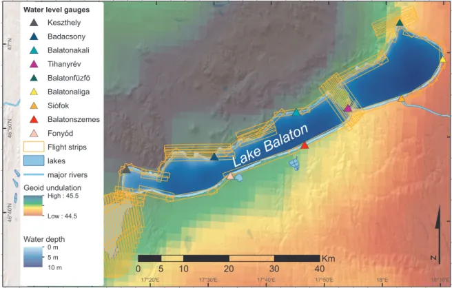
Figure 1.Map of the study area, including quasi-geoid heights, bathymetry of Lake Balaton and flight pattern. Terrain topography is repre-sented by relief shading. Note quasi-geoid high NW of the lake.
surface. While a vehicle-mounted GPS survey over the hard and quasi-stationary surface of a salt flat delivered height ac-curacies within 2.2 cm (Borsa et al., 2008b), a similar survey on a water surface encountered uncertainties in the range of 10–14 cm (Bouin et al., 2009) due to the superposition of waves and dynamic water surface height on patterns of geoid undulation.
We surveyed a lake where the surrounding gravity vari-ations are well understood and have a wide range (>1 m
quasi-geoid height range), using airborne lidar for high-resolution mapping of the lake surface height. Airborne lidar is commonly used for mapping terrain topography (Wehr and Lohr, 1999), and stationary laser altimetry has been used for time series measurements of water surface height for radar calibration (Washburn et al., 2011). Airborne lidar has also been proven to deliver height measurements comparable with satellite altimetry over sea ice and open water (Connor et al., 2009). Recently, fine-scale height differences caused by in-ternal standing waves in a coastal sea were also mapped by airborne lidar, proving that its accuracy and resolution are suitable for such studies (Magalhaes et al., 2013).
1.1 Study area
We surveyed Lake Balaton in western Hungary, which is a shallow (average depth 3.3 m), large (597 km2)and
elon-gated lake of neotectonic origin (Síkhegyi, 2002) (Fig. 1).
The geoid undulation in western Hungary increases near the axis of the Transdanubian Range, a series of hills of NE–SW orientation with elevations 600–700 m above sea level. Lake Balaton is located on the southeastern flank of this ridge; therefore the geoid undulation of its immediate neighbor-hood increases toward the northwest. This trend is explained by the isostatic unbalance of the Transdanubian Range which is a region of ongoing crustal uplift (Fodor et al., 2005; Timár et al., 2005; Síkhegyi, 2002). The center of this process is the axis of the hill chain. Repeated precise leveling has indicated maximum uplift rates of 1 mm year−1, with values between 0–0.2 mm year−1in the forelands (Joó, 1992). Other methods have suggested slightly lower uplift rates, without disputing the general trend of uplift along the hill chain axis (Szanyi et al., 2009).
2 Objectives and hypotheses
We investigated two questions and hypotheses through this case study:
(ii) Can lidar measure water surface elevation accurately enough for inferring variations in geoid undulation? Our hypothesis is that through strip adjustment based on ter-restrial target surfaces, and correction of dynamic water surface height effects, the accuracy of the measurements can be sufficient to deliver data comparable with a geoid model and suitable for inclusion in the geoid modeling process.
3 Method
Lidar (also known as Airborne Laser Scanning, ALS) is a commonly used remote sensing technique capable of rapidly surveying a large number of points with elevations and hor-izontal positions accurate to a few centimeters (Wehr and Lohr, 1999). Lidar data points are collected with direct geo-referencing, i.e., position and attitude of the scanning system are determined by GNSS (Global Navigation Satellite tem) once every second and INS (Inertial Navigation Sys-tem) data are the basis for interpolation within this time interval, separately and independently for each laser pulse. GNSS allows determining the scanner position in geocen-tric Cartesian coordinates within the reference frame of the base station. These Cartesian coordinates are first converted to ellipsoidal latitude, longitude, and height (Hoffmann-Wellenhof and Moritz, 2005) and then projected to plane grid coordinates and ellipsoidal height. This process does not in-volve a geoid model, nor is it affected by gravity variations.
3.1 Airborne data and processing
We measured elevation of the lake water surface in 58 flight strips along the whole shoreline (Fig. 2a, b). Since the main goal of the survey was littoral vegetation mapping (Zlinszky et al., 2012), the flight pattern was optimized for continuous coverage of the coast and the coastal water surface. A Le-ica ALS50 laser scanner operating at 1064 nm (Zlinszky et al., 2012, 2011) was used with a strip-wise nominal ground point density of 1 point m−2at the average flying height of
1400 m above ground level. The strip width varied between 600 and 1200 m and neighboring strips had an average over-lap of 15 %. The data were delivered in the global geodetic datum in UTM projection and this coordinate system was used throughout the study.
We used lidar strip adjustment (Filin, 2003; Kager, 2004; Ressl et al., 2011; Skaloud and Lichti, 2007) to improve the relative georeferencing of the flight strips by optimizing their relative alignment with respect to each other. In the first step, inclined planar surfaces (typically building roofs) were extracted automatically from the lidar points in each strip. During an iterative process, misalignment, lever arm, offset, scale, deflection angle, and individual global shifts of each strip were estimated in order to minimize the differences be-tween corresponding planes in the overlapping parts of each
pair of strips. The adjustment delivered optimal values for these parameters which we then used to transform all the li-dar points of each strip to new locations. The shifts were de-termined independently from eventual water-level variations as they were calculated only from selected shore features. Typical shifts were less than 20 cm.
The OPALS software package (Pfeifer et al., 2014; Mandlburger et al., 2009) was used for interpolation and processing. Moving least-squares interpolation with a plane model was applied for creating a raster elevation model of the water surface with 1 m×1 m raster resolution. We used
the lake outline and a vegetation map generated from the ALS data (Zlinszky et al., 2012) to remove the non-water areas. Visual quality control showed that cells with ellip-soidal heights lower than 149.5 m or higher than 152 m are mostly artefacts, mainly high points from vegetation, boats, etc. Therefore, cells with ellipsoidal elevations outside these limits were also excluded from further study (1 % of the lidar raster cells). As the height distribution contained some out-liers (remaining non-water points), standard deviation would not have yielded a representative value. ThereforeσMADwas
used as robust estimator of the standard deviation. It is de-fined asσMAD=1.426×MAD, where MAD is the median
of the absolute deviation to the median. For a normal distri-butionσMADis equal to the standard deviation.
3.2 Correction of dynamic water-level effects
In order to correct for short-term local water-level variations of the lake during the survey, measurements of the water gauge network around the lake were investigated. These were collected at 9 stations (Fig. 1) in 15 m intervals, using floats connected to digital recorders (3 stations) or pressure sensors (6 stations). In order to remain independent from the datum surface of the water gauges (which is a geoid model in it-self), the local mean lake level (LMLL) during the 4 flight days was calculated separately for each gauge. A time series of water-level variations compared to the LMLL was calcu-lated for each measuring station. This series was compared with GPS time recordings of each flight strip, and the ellip-soidal height of the elevation model pixels within each flight strip corrected with the difference between LMLL and local water level, measured exactly at the place and time of the strip. Correction values were between−6 and+2.5 cm, with
a median of+0.16 cm and aσMAD of 1.31 cm. As a result,
a water surface model was produced, with approximately 87 million data points characterized by horizontal coordinates and adjusted elevations above the WGS 84 ellipsoid.
3.3 Comparison with quasi-geoid model
inset
LAKE BALA
TON
18°10'E 18°5'E
18°E 17°55'E 17°50'E
17°45'E 17°40'E
17°35'E 17°30'E
17°25'E 17°20'E
17°15'E 47°5'N
47°N
46°55'N
46°50'N
46°45'N
5
km
inset
LAKE BALA
TON
5
km
Main inflow & outflow Flight strip outlines Lake Balaton shore
0 5 10 20km
a
0% 5% 10% 15%
149.65 149.75 149.85 149.95 150.05 150.15 150.25 150.35 150.45 150.55
h [m]
0% 10% 20% 30% 40%
104.9 105.0 105.1 105.2 105.3 105.4 105.5
h
corrWL- N [m]
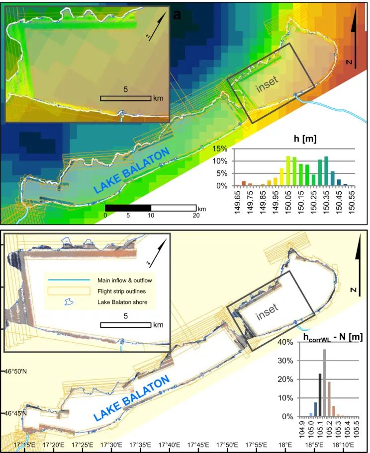
Figure 2. (a)Map of lidar-measured ellipsoidal water surface heights (inside flight strip outlines) and modeled gravity potential isosurface
height (background raster) with the same elevation color scheme. Inset shows detailed height distribution of water surface measurements,
histogram refers to lidar measurements (not to gravity potential isosurface model).(b)Map of lidar-derived normal water surface heights,
2009a, b) were considered, and HGTUB2007 was chosen due to its finer spatial resolution. We are aware that the quasi-geoid is not necessarily an equipotential surface, however, the Hungarian National Height System uses normal heights, and normal heights within Hungary deviate max. 2.8 cm from orthometric heights (Ádám, 1999), which is within lidar mea-surement accuracy. The calculation of HGTUB2007 is de-scribed in full detail in Tóth (2009b). Tóth (2009b) cal-culated the quasi-geoid from the following data sets: 6678 mean free-air gravity anomalies in 2′×3′ blocks based on
more than 300 000 point gravity data; 276 vertical deflec-tion components based on 138 astro-geodetic vertical de-flections (both north and east components); 7452 surface gravity gradients (torsion balance stations) resampled from 27 005 measurement points; and 94 GPS leveling measure-ments of the Hungarian National GPS network (OGPSH). The GPM98CR geopotential model was combined with the GRACE GGM02C model to the maximum degree and order 720 and used for reduction of the observations. RTM cor-rections were calculated based on the fixed mass model of SRTM3 heights. The residual gravity field of all observations was interpolated by least-squares collocation with the self-consistent logarithmic covariance model of Forsberg (1987), to a grid of 1.5′×1′ resolution. The estimated prediction
errors of the model are below 2 cm inside Hungary (Tóth, 2009b), which also applies to the areas near the shore that we surveyed with lidar.
For comparison with the quasi-geoid model, the lidar-derived (and water-level corrected) water surface model had to be resampled to the same spatial resolution. In order to ensure that the remaining elevated non-water points in the data do not distort the heights, the 30th percentile of the wa-ter surface model cell heights within each cell of the quasi-geoid model was calculated and used for representing the wa-ter surface heights. As a further correction, cells that did not represent the water surface height because they were mainly over shore or wetland surfaces were removed, excluding 16 of the originally 207 data points, removing the imperfections of land and vegetation masking. The correlation of this low-resolution water surface height model with the quasi-geoid was tested by linear regression.
4 Results
The 87 077 358 water surface model raster cells had an lipsoidal elevation range of 80 cm (Fig. 2a). The largest el-lipsoidal elevations of the water surface are in the north-western basin of the lake, decreasing gradually toward the southern shore with the lowest areas in the eastern corner (see supplementary data for high-resolution map). The ellip-soidal heights of the water surface in overlapping areas of strips surveyed on different days were similar within the ac-curacy range of the instrument (<8 cm, Leica Geosystems
AG, 2006). Water levels measured during the flight window
44.65 44.70 44.75 44.80 44.85 44.90 44.95 45.00 45.05 45.10 45.15 45.20 45.25 45.30 149.60
149.65 149.70 149.75 149.80 149.85 149.90 149.95 150.00 150.05 150.10 150.15 150.20 150.25 150.30 150.35 150.40 150.45 150.50 150.55 150.60
Quasi-geoid height [m]
ALS-measured ellipsoidal water surface height [m]
Point count
1:1 line
1
2 - 5
6 - 10
11 - 50
51 - 75
76 - 125
126 - 225
226 - 430
431 - 850
851 - 1,700
1,701 - 3,350
3,351 - 6,700
6,701 - 13,500
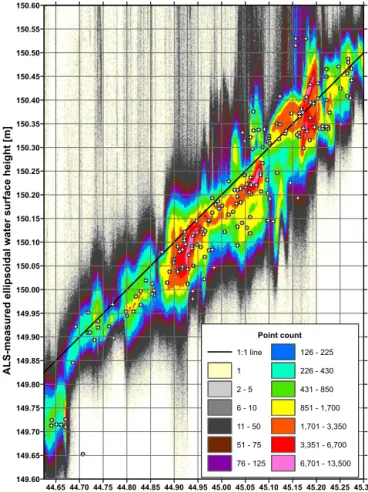
Figure 3. Scatterplot of water surface ellipsoidal heights (cor-rected with deviation of local water level from LMLL) with respect to local quasi-geoid height. Scatterplot cell coloring shows point count for each ellipsoidal water height/quasi-geoid height interval
of 1.25×1.25 cm. Bilinear interpolation of geoid undulation raster
to lidar height model resolution was used for this graph. Crosses show water surface and quasi-geoid height data points resampled to quasi-geoid model resolution as used for calculating regression.
showed some variation (explained in detail in Appendix A), with a total range of 20 cm for all stations. Water-level devi-ations from LMLL measured synchronously with the flight strips have a total range of ±6.0 cm for the 4 flight days
(Fig. 4).
# * #* # * # * # * # * # * # * # * 18°E 17°50'E 17°40'E 17°30'E 17°20'E 18°10'E 4 6 °4 0 'N 46°50'N 46°40'N
Day 1 Day 2 Day 3 Day 4
$
0 5 10 20 30 40 Km -10 -5 0 5 10 0 0 :0 0 0 6 :0 0 1 2 :0 0 1 8 :0 0 0 0 :0 0 0 6 :0 0 1 2 :0 0 1 8 :0 0 0 0 :0 0 0 6 :0 0 1 2 :0 0 1 8 :0 0 0 0 :0 0 0 6 :0 0 1 2 :0 0 1 8 :0 0 -5 5 -5 5 -5 5 -5 5 -5 5 -5 5 -5 0 5 -5 5 w l - L M L L [ c m ]
Figure 4. Water-level recordings with respect to LMLL of all 9 water-level gauges around Lake Balaton, during the 4 flight days. Triangles in the map depict the water gauges (colour coded to the water level graphs), rectangles crossing all graphs show actual flight times of lidar strips.
height range of the water surface heights was approximately 80 cm, with a dispersion (quantified by σMAD) of 20 cm
(Fig. 2a). The water surface heights resampled to the quasi-geoid model resolution were compared with the quasi-quasi-geoid height of each cell: a linear regression with an R2 value
of 0.906 was calculated with a slope of 1.12, intercept of 99.95 m andσMAD of 5.17 cm. This agrees with our
expec-tation that the pattern of water surface ellipsoidal heights is explained by the height variations of the gravity potential iso-surface.
When the local quasi-geoid heights were resampled by bi-linear interpolation to the spatial resolution of the water sur-face model (1 m×1 m) and subtracted from the local water
surface model elevations, theσMAD was reduced to 5.6 cm,
and the elevation range of the water points to 30 cm. 78 % of the points were within 15 cm and 36.1 % of the 87 077 358 points within 5 cm (Fig. 2b). Hardly any flight strips show along-track differences, not even those spanning 15 cm of quasi-geoid height range along their length (across-track dif-ferences are mainly artefacts discussed in Appendix B). The geoid-corrected water surface heights are slightly lower than
average in the SE corner of the lake and higher than average in the NW, a pattern that suggests that the height gradient of the lake may be even steeper than the gradient in the quasi-geoid model.
This is confirmed by the scatterplot of the measured el-lipsoidal water surface heights and the corresponding geoid undulation (Fig. 3). A clear linear trend is visible, and the slope is very close to 1 (1.06), which agrees with our expec-tation that the geoid undulation controls water surface height variation in space. Nevertheless, water surface heights show a steeper profile than the geoid model, and fall clearly below the 1:1 line for the lowest quasi-geoid height values.
Erro-neously high or low artefact points are probably created by insufficiently removed non-water features and by waves.
5 Error budget
5.1 Relative georeferencing
For the lidar data of Lake Balaton no geometric ground con-trol features were available, therefore the absolute georefer-encing accuracy is a product of standard differential GNSS georeferencing (10 cm according to the flight operator), en-hanced by the large number of measurements. However, the relative georeferencing of the strips (i.e., their mutual align-ment) was improved by strip adjustment, as documented by
σMADof the differences in smooth areas of overlapping strip
pairs. For all considered 305 pairwise strip differences (with around 106 000 000 difference values in total) σMAD
im-proved from 12 cm (before) to 5 cm (after strip adjustment).
5.2 Dynamic water-level correction
Single water gauge measurements can be considered accu-rate within 1 cm, but the LMLL as a datum surface is slightly less accurate. Calculated as an average of the local water lev-els measured every 15 min during the 4 flight days, the er-rors of LMLL can be estimated from the range of local mean water levels calculated separately for each measurement day and each gauge. This is below 2 cm for all stations, and below 1 cm for 6 out of 9 stations.
A possible source of error in the height measurements was water as the target surface for lidar. Water is not a strong reflector at the wavelength used (1064 nm). The nature of re-flection from the surface or penetration into the water col-umn depends strongly on the look angle, therefore from dif-ferent parts of the strips either no points were recorded, ac-curate measurements were made or (rarely) erroneously long or short ranges were measured. A detailed overview of the artefacts produced by water as a target surface and how this affected our measurements is provided in Appendix B.
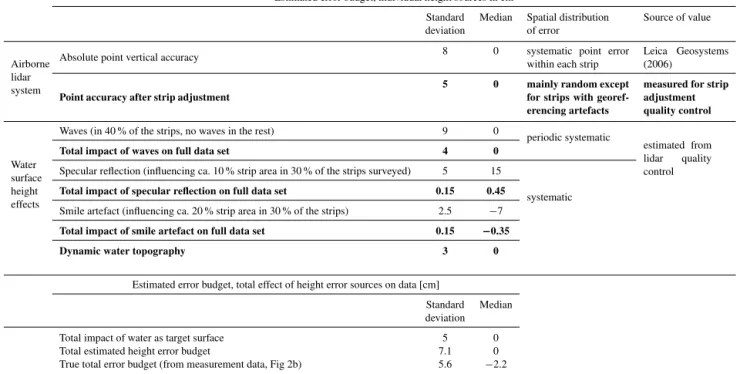
Table 1.Error budget, including standard deviation and median of each individual error source and the theoretical error propagation, com-pared with the dispersion found in the measurement data. Lines indicated in bold influence the final error budget. Lines not in bold show intermediate calculation steps, they only apply to the theoretical case without strip adjustment (Absolute point vertical accuracy) or to the individual strips affected by water artefacts. The total impact of water artefacts was calculated by averaging these values across the total data set.
Estimated error budget, individual height sources in cm
Standard Median Spatial distribution Source of value deviation of error
Airborne lidar system
Absolute point vertical accuracy 8 0 systematic point errorwithin each strip Leica Geosystems(2006)
Point accuracy after strip adjustment
5 0 mainly random except for strips with georef-erencing artefacts
measured for strip adjustment quality control
Water surface height effects
Waves (in 40 % of the strips, no waves in the rest) 9 0
periodic systematic
estimated from lidar quality control Total impact of waves on full data set 4 0
Specular reflection (influencing ca. 10 % strip area in 30 % of the strips surveyed) 5 15
systematic Total impact of specular reflection on full data set 0.15 0.45
Smile artefact (influencing ca. 20 % strip area in 30 % of the strips) 2.5 −7
Total impact of smile artefact on full data set 0.15 −0.35
Dynamic water topography 3 0
Estimated error budget, total effect of height error sources on data [cm]
Standard Median deviation Total impact of water as target surface 5 0 Total estimated height error budget 7.1 0 True total error budget (from measurement data, Fig 2b) 5.6 −2.2
average) and low current intensity at the time of flight. Never-theless, a number of processes with proven effects in marine settings which might also potentially influence the height of the water surface in our case are discussed below:
5.3 Seiche and setup
Storms can produce disequilibrium of the lake surface, in-creasing the water level on the downwind side while decreas-ing it upwind (setup) or producdecreas-ing dynamic standdecreas-ing waves along or across the lake, with wavelengths of several kilo-meters (seiche). In case of Lake Balaton, this starts at sus-tained wind speeds above 5 m s−1and such a displacement can reach 1 m in water level during storms winds of 20 m s−1 (Muszkalay, 1973; Somlyódy, 1983). According to local Me-teorological Aerodrome Report (METAR) data, wind speeds never exceeded 5 m s−1during the whole survey. Some setup
and seiche effects can be observed in the water-level data (see Appendix A and Fig. 4), but these were corrected for as described in the methodology. The remaining uncertainty of the dynamic water topography correction is a consequence of using the difference of LMLL of the nearest gauge for each strip. In the worst possible case, this might produce an error in range of the difference in deviation of LMLL between two neighboring gauges. These differences had a standard devia-tion of 3 cm for the 4 flight days (Table 1).
5.4 Currents
On Lake Balaton, currents are driven by wind forcing and by seiche while thermal convection remains hardly observ-able (Muszkalay, 1973). The flow of water from the tribu-taries towards the outlet is also very weak, because signif-icantly more water leaves the lake through surface evapo-ration than through the outflow. The patterns observed in ellipsoidal height do not match the main tributaries or the outlet of the lake, ruling out river plumes. Current flow can locally reach 1 m s−1 in cases of storms or strong seiche
(Virág, 1998). While no direct current measurements have been carried out during our survey, the wind speeds were low (<5 m s−1) as documented by the METAR reports, and
se-iche displacements were within a few centimeters as detailed in Appendix A. Therefore we have a reason to believe cur-rents were negligible.
5.5 Waves
does not contribute to the lake-scale pattern of ellipsoidal height that we derive our conclusions from, as wind-induced waves involve a periodic motion of water with equal am-plitudes below and above the mean water level (Imboden, 2003).
5.6 Air pressure response
The rule of thumb for air pressure response is 1 cm decrease in water level for 1 mbar increase in air pressure (Ponte and Gaspar, 1999). However, this only applies to the open ocean and after a period of 1–2 weeks. In our case, since the flights took place within 10 days and since the lake was very shal-low, most of the air pressure is directly forwarded to the lake bottom. Therefore we assume that air pressure changes could not have influenced the local lake level by more than a few millimeters during the measurement.
5.7 Lake Tides
Lake tides are known to have amplitudes of up to 10 cm in larger lakes (Trebitz, 2006). In case of Lake Balaton, the shal-low depth and the relatively shal-low water volume of the lake suggest this effect would be even smaller. During long-term investigation of water movements conducted in the 1970’s, no evidence of lake tides was observed (Muszkalay, 1973), therefore we do not expect these to have influenced lake level.
5.8 Density change
Due to its fresh water, shallow depth (3.3 m avg), limited in-flow and small water volume (2 km3) compared to its
sur-face (600 km2), Lake Balaton experiences very limited
vari-ations in water density. There is no thermocline, warming and cooling can only create maximum vertical temperature gradients of up to 1.1◦C m−2, and horizontal differences in
surface temperature between basins have been documented to remain less than 3◦C (Virág, 1998). The salinity of the
water is also quite constant over its area and over time, so no major changes in density are expected. The height effect of local warming or cooling can dissipate relatively quickly on this scale, therefore no contribution of density change to lake topography can be expected.
5.9 Summary of error budget
The most important errors influencing our data are summa-rized in Table 1. In case of the single lake surface height cells in the raw data, the most important source of height er-ror is the combination of GNSS positioning and lidar range measurement, causing errors around 8 cm (Leica Geosystems AG, 2006). With strip adjustment this quality can be assured and even improved, as in our case the differences between overlapping surface model heights (on land) showed a stan-dard deviation of 5 cm. This is the sensor-based uncertainty
in each of our water surface model cells (the water surface model is defined in Sect. 3.2).
The effects of water as a target surface are discussed in de-tail in Appendix B. Each lidar strip was inspected for such effects, and the typical amplitude and the size of the af-fected area noted. Waves were only encountered in part of the strips, and their amplitudes were low. Specular reflection influenced a very narrow part of some strips at nadir, creating systematic positive shifts in these data cells, but these have a very low proportion relative to the full data set. ”Smile” artefacts (discussed in Appendix B again) were mutually exclusive with waves and specular errors, and produced a systematic negative shift at some strip edges. Dynamic wa-ter topography is expected to have produced errors within 3 cm standard deviation.
The total theoretical impact of water as a target surface can be calculated by summing the error distributions and calcu-lating the median and the standard deviation of the result. No systematic shift in the data is expected here, since the system-atic errors affecting the median are rare and low. The 5 cm standard deviation is mainly caused by waves and dynamic water topography. The total estimated height error budget ad-ditionally includes the post-adjustment relative georeferenc-ing error.
The distribution of our water surface model heights cor-rected with the local quasi-geoid height (which also has a 2 cm standard deviation) shows a smaller deviation than the-oretically expected from the inspected error sources. The
−2 cm bias in absolute height (compared to the 105.19
of-ficial water level measured at Siófok during the flight days) may be caused by remaining absolute inaccuracies of the GNSS positioning (which is only partly corrected by strip adjustment) and uncertainties of water-level measurements. In the future, for such surveys, measuring of ground control points is highly advisable in order to avoid the eventual ab-solute error of GNSS.
If the data is to be used for geoid modeling, the error bud-get could be improved by two factors: automatic removal of specular and smile effects (see Sect. 6.2), and interpolation of water surface height into larger cells, removing periodic and some random error.
6 Discussion and outlook
of water during the flight period were corrected for. One of the limitations of investigating this correlation is the resolu-tion of the quasi-geoid model we used: similar to satellite al-timetry, the resolution of the water surface is much higher than the resolution of the geoid model, therefore limiting comparison (Cheng et al., 2008). The high resolution of the lidar-derived water surface model shows short-wavelength patterns in height, and therefore potentially in geoid undu-lation, which are beyond the scale of the quasi-geoid model we used, and indeed most geoid models available. This im-plies that water surface ellipsoidal heights measured by lidar might be used in the future to refine local gravity variation models.
6.1 Comparison with other measurement methods The theory of hydrostatic equilibrium being connected over large areas to the local gravity field has already been utilized for surveying the geoid over the oceans (such as ICESat and Envisat), but these measurements are affected by dynamic ocean topography (Hoffmann-Wellenhof and Moritz, 2005). In our case, the dense network of water-level gauges and the high measurement frequency allowed quantification of dy-namic water height effects and correction of any measure-ment bias. This was possible since only water surfaces close to the shore were surveyed and because the flight took place under calm weather conditions. Our lidar measurement accu-racy of 5 cm calculated from flat terrestrial surfaces after strip adjustment compares to the 4 cm accuracy obtained by Borsa et al. (2008b) through vehicle-mounted GPS surveys (over much larger area), and to the best accuracies measured from ship-mounted GPS under calm weather conditions (10 cm) (Bouin et al., 2009), but are slightly worse than the 2.7 cm error reached with a GPS catamaran in a marine setting by Bonnefond et al. (2003). Borsa et al. (2008a) find that 93 % of the ellipsoidal height variations of a dry salt flat are explained by variations in geoid height, and come to the conclusion that the surface topography closely approximates the gravity equipotential surface. At the scale of the most detailed quasi-geoid model we could obtain, we found that 90.1 % of the water surface topography variation is explained by variations in quasi-geoid height.
Point elevation measurements from GNSS buoys were al-ready used as part of a leveling-based geoid survey (Gomez et al., 2013), and satellite gravimetry-based geoid change measurements have been used as a proxy for lake water levels (Awange et al., 2008; Calmant et al., 2008). However, active satellite altimeters were only applied in rare cases for map-ping inland lakes as level surfaces, probably mainly because of their limited spatial resolution (Hoffmann-Wellenhof and Moritz, 2005; Cheng et al., 2008; Baghdadi et al., 2011).
Comparing satellite altimetry with terrestrial, airborne and satellite gravimetry over the Great Lakes, Kingdon et al. (2008) observe that lake surface altimetry follows short-wavelength gravity anomalies confirmed by ship- or airborne
gravimetry better than a lower resolution model based on GRACE satellite data does. They also describe the absolute accuracy of the altimetry-derived quasi-geoid to be closer to the GRACE values than the high-resolution ship- or air-borne measurements, which were more prone to systematic bias. This means that altimetry was more accurate than ter-restrial gravimetry but delivers higher resolutions than satel-lite gravimetry. If the same principles apply to lidar, which is also based on altimetry, it can be expected that lidar-derived lake surface heights would deliver a valuable input to high-resolution geoid models. Compared to satellite altimetry, li-dar is characterized by smaller footprints, even higher spatial resolutions and the possibility to survey large areas within a few hours. Similarly to satellite altimetry over oceans, the spatial resolution and area coverage of lidar could theoreti-cally allow identification of dynamic water topography fea-tures of lakes such as plumes or eddies. Since our data only covered the waters nearest to the shore, and since the lake was near equilibrium, this could not be tested in our case.
Compared to GPS buoys which collect height data spread over longer periods to assess mean lake level, lidar deliv-ers repeated measurements spread in space. This has com-parable accuracy to the technique of Bonnefond et al. (2003) who used GPS receivers mounted on a ship to obtain area-covering sea level height measurements, but is more produc-tive due to higher survey speeds and area coverage. However, lidar surveys provide a snapshot and are thus more easily dis-torted by the effects of water movement, requiring correction based on local water stages. The method we proposed only needs relative height changes at each gauge.
Compared to analysis of simultaneous water-level gauge readings such as Cheng et al. (2008), the advantage of lidar in our case is the higher number of data points, which de-liver statistically stronger results while using coverage of the shore for accurate relative georeferencing. It is expected that in the future, lidar coverage of lake surfaces will further in-crease with the spread of bathymetric lidar (Mandlburger et al., 2011).
6.2 Outlook: including water surface lidar heights in geoid modeling
The full process of creating a new local quasi-geoid model including water surface height data from lidar and the eval-uation of this quasi-geoid map would be outside the scope of the current paper. However, we believe that in the fu-ture, lidar-derived lake surface data can be used in a way similar to GPS-leveling data: lidar provides an ellipsoidal height while local water gauges provide (in the Hungarian case) the normal height of the same object, the water sur-face. In practice, the following steps (beyond those already described in the methods section) are recommended: any data points where elevation can be considered uncertain from vi-sual inspection should be excluded (surface glint, smile ef-fects, twist); lidar data points should be aggregated to larger raster cells (eg. 100×100 m, 10 000 points), which also
fur-ther reduces error; the leveling of the water gauges should be checked and any biases corrected; and for each lidar-derived raster cell, the local water stage should be interpolated from timed water-level records and proximity to gauges. After these steps, the quasi-geoid height of each raster cell can be calculated from the difference between ellipsoidal (lidar) and normal (gauge) water surface height and can be loaded to the least-squares collocation for the geoid model together with other data types. Lidar mapping of lake surface elevations can deliver information on the ellipsoidal height pattern of the water surface, and thus on the local gravity anomalies. These in turn can be used to collect information about the formation of the lake (Dietrich et al., 2013). Lidar survey-ing of lakes can be valuable for estimatsurvey-ing the error budget of lower resolution regional geoid models and GPS-derived heights based on such models. Since many major European and North American lake shores have already been surveyed by lidar, there is a wealth of data available.
7 Conclusions
We conclude that a lake may reach a level of hydrostatic equi-librium that allows it to be used as a basis for mapping a grav-ity potential isosurface. This can be assessed on the basis of water gauge readings, which can also be used to correct the remaining lake-scale dynamic surface topography. The ellip-soidal height of the lake surface has been proven to closely follow the local geoid undulation, within the limits of instru-ment accuracy and quasi-geoid model resolution.
Appendix A: Water levels of Lake Balaton during the studied period
Investigation of the water levels of the lake will be used to answer two questions:
(i) To what extent was the lake at hydrostatic equilibrium during the airborne survey?
(ii) How did variations in local lake water levels affect the ellipsoidal heights measured by lidar?
Hydrostatic equilibrium would mean that the lake was free from dynamic processes such as local currents, eddies and standing waves, and therefore the rules of hydrostasis would govern the pattern of its surface elevation. Whether the lake was in such a state can be determined by local water-level variations. The common datum of water gauges around the lake was determined by a geoid model, therefore it is subject to errors of the model and might not perfectly represent the true long-term surface of the lake in theoretical equilibrium. Therefore, we studied water-level changes independently for each gauging station: LMLLs for each station are expected to define this equilibrium across long-term measurements. Dur-ing the four flight days, the daily LMLLs showed increases or decreases of a few centimeters, consequently it was assumed that slight changes of lake water volume were affecting these measurements (Fig. 4). In this case, measuring LMLL across longer periods of time might not necessarily have increased the accuracy of LMLL estimation.
While wind and currents of lakes are known to induce static and also periodic deviations from the equilibrium wa-ter level (setup and seiche), the wind speeds observed dur-ing the campaign were below the known threshold for such processes (Muszkalay, 1973). The flight data was collected during 21, 22, 23 and 26 August 2010. August 24 and 25 were left out because of cloudy weather. During Day 1, the highest water level, 122 cm above the station datum (8 cm above LMLL) was observed in Keszthely, where the water level slowly fluctuated between 112 and 122 cm with a period of ca. 5 h. While this periodic fluctuation with decreasing amplitude implies a standing wave (seiche), no water gauge showed the same movement in the opposite direction. It is already known that the Keszthely gauge typically records the largest dynamic water-level variations, since the small west-ern basin of the lake is the most sensitive to the wind. This fluctuation was most probably caused by remnants of seiche from winds during the previous day (Fig. 4).
The lowest water level for Day 1, 103 cm (9 cm below LMLL) was observed in Tihanyrév in the Tihany straits and is an isolated low record both preceded and followed by continuous recordings around 111 cm (0.7 cm below LMLL). This pattern matches some measurements described by Muszkalay (1973) as a short-term standing wave formed within a harbor basin, which might well be the case since Tihanyrév has intensive ferryboat traffic. Neither of these de-viations corresponded to the flight times of Day 1; in fact,
during the afternoon flight the water level was within 2 cm of LMLL for all stations near the flight area of the day (Fig. 4). During Day 2, the highest recorded water-level deviation was 5 cm above the LMLL, again an isolated measurement of 117 cm in Tihanyrév preceded and followed by values around 112 cm. The lowest level was 1.9 cm below LMLL, 110 cm measured at Siófok, preceded and followed by readings of 111 cm. During the time of the flight on that day, the devi-ation from LMLL was between−1.8 and+2.3 cm for the
stations covered by the flight area (Fig. 4).
During Day 3, the highest differences of LMLL of
+3.3 cm were measured over the course of an hour in the
evening in Balatonf˝uzf˝o, not counting an isolated reading of
+4.2 cm in the Tihanyrév harbour. The largest negative
dif-ference of LMLL was−2.9 cm in Siófok, sustained during
several hours at night. The minimum of−2.7 cm compared to
LMLL (111 cm above gauge datum) was continuously mea-sured during the morning hours of the day in Keszthely. Dur-ing the flight, deviations from LMLL were between−1.8 and +3.3 cm (Fig. 4).
During Day 4, the largest absolute differences with re-spect to LMLL were+10.3 and−7.7 cm, both observed in
Keszthely. Here the water level rose from 114 cm (above the gauge datum) to 124 cm over 2 h and fell back to 112 over the next two hours. The largest negative deviation (−7.7 cm)
happened during the flight in Keszthely, the largest positive difference in LMLL was+2.1 cm in Siófok (Fig. 4).
Apparently, even under calm conditions, standing waves and other dynamic processes can cause up to 10 cm differ-ences compared to the average water level. The strongest fluctuations were observed in Keszthely and Balatonf˝uzf˝o, which are both near the ends of the lake and in narrow cor-ners capable of producing water level changes higher than on the open lake surface due to a funnel effect. If this is the case and the lake level changes amplified by the funnel ef-fect reach no more than 10 cm compared to the average wa-ter level, we can only expect minor dynamic lake topography along the more open shores. We thus conclude that while the lake was not at full hydrostatic equilibrium during the flight days, dynamic local water level changes were within
±5 cm for most measurement sites and within±10 cm
glob-ally. Due to high frequency water-level measurements and some luck in the afternoon timing of most flights, the dy-namic water-level variations actually affecting our measure-ments were even lower, typically within±3 cm, in one
iso-lated case reaching−7.7 cm. These variations were relatively
well understood and corrected for by measuring deviations from LMLL at 9 stations with 15 min frequency.
Appendix B: Possible sensor artefacts due to water as a target surface
column and is absorbed, since water is a weak reflector at the near-infrared wavelength we used (1064 nm). Some of the pulse energy can nevertheless be scattered back to the sensor from below the water surface. The rest of the light is reflected from the surface, part of it with near-Lambertian characteris-tics, part of it specularly. In case of specular reflection, very high amounts of radiation are reflected back into the sensor at nadir, while off-nadir, the energy is reflected away from the sensor and none of it is received. In case of waves, every crest may have a surface inclined to produce a specular re-flection towards the sensor. However, given a constant wave amplitude, chances for a reflection towards the sensor will decrease with increasing look angle.
The proportions of light absorbed, volume scattered, spec-ularly reflected and scattered from the water surface depend on sensor wavelength, the optical characteristics of the wa-ter, the roughness and inclination of the water surface and the look angle of the outgoing pulse, discussed in detail in Guenther et al. (2000).
In case of very flat water, the pulse energy is reflected away from the sensor for most of the strip, with an insufficient return for triggering the detector and therefore no recorded point. At nadir and again over calm water, the pulse energy reflected specularly arrives back in the sensor, producing a point and also often a glint effect with very high echo inten-sity. This is known to result in slightly shorter range mea-surements (10–50 cm), as the high amount of incoming en-ergy causes the system to detect a peak too early (range-walk effect). Obvious glint range-walk effects were encountered in less than 1 % of the data (see histogram in Fig 2b), since for most of the areas where the water surface was completely flat, no points were registered as described above.
For most of the flight campaign, moderate waves were en-countered. These were sufficient to produce non-specular re-flection over most of the covered strip surface, but no data points were produced closer to the edges of the strips due to a combination of water absorbing the pulse energy and semi-specular reflection away from the sensor. The width of this “blank” edge again varies depending on local water surface characteristics. Closer to the strip centerline, but still nearer to the edge of the strip, slight decreases of the heights from the strip center to the strip border by about 5 cm (Fig. 2a, supplementary material) can be observed in some cases. This small systematic smile error may have two causes:
(i) The most likely reason for this observed smile error may lie in the interaction of the laser signal with the water surface as explained above. That is, perhaps in this part of the affected strips the pulse energy entered the water, and volume scattering of water contributed to the re-flected energy besides surface reflection, and thus pro-duced a measurement of erroneously long range, i.e., low water surface. The width of this “too-low” part of the strip is usually not more than 100 m.
(ii) With increasing look angle the portion of specular re-flected energy away from the sensor increases, thus ever less energy is detected by the sensor. Since very high amounts of incoming energy (in the nadir) cause the system to detect a peak too early (resulting in too-short ranges), it seems logical that with decreasing amounts of incoming energy the system will detect a peak too late (resulting in too-long ranges; i.e., low water sur-face). The width of this too-low part of the strip is usu-ally not more than 100 m. Having systematicusu-ally in-spected each flown strip for the “empty edge”, smile, specular center and wave effect, the following conclu-sions were made:
The width of the strip edges where no lidar echo from wa-ter was observed was typically 200 m on either side of the strip, and all lidar strips collected were affected by this. This varied by about 50 m depending on surface conditions, with narrower empty strips where waves were encountered, and exceptionally very broad empty strips where water was com-pletely flat and specular reflection dominated. This suggests that the empty edge effect is caused by the dominance of specular reflection and absorbance above a certain angle of incidence between the pulse and the water surface.
Over completely flat water, in our case in the wind shadow of terrain (west of the Tihanyrév gauge and area around the Badacsony gauge), specular reflection dominated. Up to 15– 20 cm overestimations of water surface height due to specu-lar effects were observed in small parts of 20 of the 58 strips we used. All of these were in very calm water conditions. In some extreme cases (5 strips) the strip area would be com-pletely empty except for the very narrow (5–20 m) centreline where points would have erroneous heights due to specular effects; implying that specular reflection dominated in these cases and data were only collected at nadir.
The artefact of erroneously low strip edges (smile) was encountered in 19 of the 58 strips, all of these in the eastern basins of the lake where the water is less turbid than in the west. Most strips are completely free from this artefact, sug-gesting no systematic internal errors of the scanning system were encountered. The affected strips were all on the north-ern shore in deep water and local wind shadow, again imply-ing low turbidity. The smile effect typically occurred at scan angles near 20◦, which follows our expectation that the entry
of the laser pulse into the water column is limited to a certain angle of incidence (a fact well known in the bathymetric lidar domain).
A further, final cause of strip patterns may lie in remain-ing errors of the strip adjustment process. Durremain-ing survey-ing, a sensor problem was discovered to affect the data: the central position of the scanning mirror was determined with some uncertainty, resulting in a slight “twist” of the affected data strips along their longitudinal axis, with erro-neously low cells on one edge and erroerro-neously high on the other (+/−5 cm). Strip adjustment corrected this effect as
described in the text, but in some rare cases (definitely not more than 7 of our 58 strips), the low overlap with other strips means that some such error may have remained.
The Supplement related to this article is available online at doi:10.5194/se-5-355-2014-supplement.
Acknowledgements. The airborne survey of the lake was spon-sored by the European Community’s 7th Framework Programme (FP7/2008-20012) under EUFAR contract no. 2271; strip adjustment was funded by the GIONET FP7 project (PITN-GA-2010-264509). A. Zlinszky and partly B. Székely and N. Pfeifer were funded by the Changehabitats2 FP7 project, C. Briese by the Ludwig Boltzmann Institute, B. Székely contributed as an Alexander von Humboldt Research Fellow. Contribution of G. Timár was partially supported by the Hungarian National Re-search Fund (OTKA) project NK83400, A. Zlinszky was partially supported by the project TÁMOP-4.2.2.A-11/1/KONV-2012-0064 “Regional effects of weather extremes resulting from climate change and potential mitigation measures in the coming decades”. The HGTUB2007 geoid model was kindly provided by Gyula Tóth from the Department of Geodesy and Surveying of the Budapest University of Technology and Economics.
Edited by: A. Jordán
References
Ádám, J.: Difference between geoid undulation and quasigeoid height in Hungary, Bolletino di Geofisica Teorica e Applicata, 40, 571–575, 1999.
Awange, J. L., Sharifi, M. A., Ogonda, G., Wickert, J., Grafarend, E. W., and Omulo, M. A.: The falling Lake Victoria water level: GRACE, TRIMM and CHAMP satellite analysis of the lake basin, Water Resour. Manage., 22, 775–796, 2008.
Baghdadi, N., Lemarquand, N., Abdallah, H., and Bailly, J. S.: The Relevance of GLAS/ICESat Elevation Data for the Monitoring of River Networks, Remote Sens., 3, 708–720, 2011.
Bonnefond, P., Exertier, P., Laurain, O., Menard, Y., Orsoni, A., Jeansou, E., Haines, B. J., Kubitschek, D. G., and Born, G.: Lev-eling the Sea Surface Using a GPS-Catamaran, Marine Geodesy, 26, 319–334, 2003.
Borsa, A. A., Bills, B. G., and Minster, J.-B.: Modeling the topog-raphy of the salar de Uyuni, Bolivia, as an equipotential surface of Earth’s gravity field, J. Geophys. Res.-Solid Earth, 113, 1–21, 2008a.
Borsa, A. A., Fricker, H. A., Bills, B. G., Minster, J.-B., Caraba-jal, C. C., and Quinn, K. J.: Topography of the salar de Uyuni, Bolivia from kinematic GPS, Geophys. J. Internat., 172, 31–40, 2008b.
Bouin, M.-N., Ballu, V., Calmant, S., Bore, J.-M., Folcher, E., and Ammann, J.: A kinematic GPS methodology for sea surface map-ping, Vanuatu, J. Geodesy, 83, 1203–1217, 2009.
Brettenbauer, K. and Weber, R.: A primer of geodesy for GIS users, Geowissenschaftliche Mitteilungen, 64, 1–55, 2003.
Calmant, S., Seyler, F., and Cretaux, J. F.: Monitoring Continental Surface Waters by Satellite Altimetry, Surv. Geophys., 29, 247– 269, 2008.
Cheng, K.-C., Kuo, C.-Y., Shum, C. K., Niu, X., Li, R., and Bed-ford, K. W.: Accurate linking of Lake Erie water level with
shore-line datum using GPS buoy and satellite altimetry, Terrestrial At-mos. Oc. Sci., 19, 53–62, 2008.
Connor, L. N., Laxon, S. W., Ridout, A. L., Krabill, W. B., and McAdoo, D. C.: Comparison of Envisat radar and airborne laser altimeter measurements over Arctic sea ice, Remote Sens. Envi-ron., 113, 563–570, 2009.
Del Cogliano, D., Dietrich, R., Richter, A., Perdomo, R., Hor-maechea, J. L., Liebsch, G., and Fritsche, M.: Regional geoid determination in Tierra del Fuego including GPS levelling, Geo-logica Acta, 5, 315–322, 2007.
Dietrich, V. J., Lagios, E., Reusser, V., Sakkas, E., Gartzos, E., and Kyriakopoulos, K.: The enigmatic Zerelia twin-lakes (Thes-saly, Central Greece): two potential meteorite impact craters, Solid Earth Discuss., 5, 1511–1573, doi:10.5194/sed-5-1511-2013, 2013.
Filin, S.: Recovery of systematic biases in laser altimetry data using natural surfaces, Photogramm. Engin. Remote Sens., 69, 1235– 1242, 2003.
Fodor, L., Bada, G., Csillag, G., Horváth, E., Ruszkiczay-Rüdiger, Z., Palotás, K., Síhegyi, F., Timár, G., Cloetingh, S., and Horvath, F.: An outline of neotectonic structures and morphotectonics of the western and central Pannonian Basin, Tectonophysics, 410, 15–41, 2005.
Forsberg, R.: A new covariance model for inertial gravimetry and gradiometry, J. Geophys. Res.-Solid Earth Planet., 92, 1305– 1310, 1987.
Gomez, M. E., Del Cogliano, D., and Perdomo, R.: Geoid mod-elling in the area of Fagnano Lake, Tierra del Fuego (Argentina): insights from mean lake-level observations and reduced gravity data, Acta Geodaetica et Geophysica, 48, 139–147, 2013. Guenther, G. C., Cunningham, A. G., LaRocque, P. E., and Reid, D.
J.: Meeting the accuracy challenge in airborne lidar bathymetry, EARSel, Dresden, 2000.
Hipkin, R.: Modelling the geoid and sea-surface topography in coastal areas, Phys. Chem. Earth Part A, 25, 9–16, 2000. Hoffmann-Wellenhof, B. and Moritz, H.: Physical Geodesy,
SpringerWienNewYork, Wien, Austria, 397 pp., 2005.
Imboden, D. M.: The motion of Lake Waters, in: The lakes hand-book, edited by: Reynolds, C. S., and O’Sullivan, P., Blackwell, Oxford, 115–152, 2003.
Joó, I.: Recent vertical surface movements in the Carpathian Basin, Tectonophysics, 202, 129–134, 1992.
Kager, H.: Discrepancies between overlapping laser scanning strips – Simultaneous fitting of Aerial Laser Scanning strips, Interna-tional Society for Photogrammetry and Remote Sensing XXth Congress, Istanbul, 2004/07/12, 2004.
Kenyeres, A.: Completion of the nationwide GPS-gravimetric geoid solution for Hungary, Phys. Chem. Earth Part A, 24, 85–90, 1999.
Kingdon, R., Hwang, C., Hsiao, Y.-S., and Santos, M.: Gravity anomalies from retracked ERS and Geosat altimetry over the Great Lakes: Accuracy assessment and problems, Terrest. At-mos. Oceanic Sci., 19, 93–101, 2008.
Magalhaes, J. M., da Silva, J. C. B., Batista, M., Gostiaux, L., Gerkema, T., New, A. L., and Jeans, D. R. G.: On the detectabil-ity of internal waves by an imaging lidar, Geophys. Res. Lett., 40, 3429–3434, 2013.
modelling, Hydrol. Earth Syst. Sci., 13, 1453–1466, 2009, http://www.hydrol-earth-syst-sci.net/13/1453/2009/.
Mandlburger, G., Pfennigbauer, M., Steinbacher, F., and Pfeifer, N.: Airborne Hydrographic LiDAR Mapping – Potential of a new technique for capturing shallow water bodies, 19th Interna-tional Congress on Modelling and Simulation, edited by: Chan, F., Marinova, D., and Anderssen, R. S., 2416–2422, 2011. Merriman, M.: Figure of the Earth – an introduction to geodesy,
John Wiley & Sons, New York, 88 pp., 1881.
Muszkalay, L.: A Balaton vizének jellemz˝o mozgásai,
Vízgazdálkodási Tudományos Kutató Intézet, Budapest, 85 pp., 1973.
Pfeifer, N., Mandlburger, G., Otepka, J., and Karel, W.: OPALS – A framework for Airborne Laser Scanning data analysis, Comput-ers, Environ. Urban Syst., 45, 125–136, 2014.
Ponte, R. M. and Gaspar, P.: Regional analysis of the inverted barometer effect over the global ocean using TOPEX/POSEIDON data and model results, Journal of Geo-physical Research: Oceans (1978–2012), 104, 15587–15601, 1999.
Ressl, C., Pfeifer, N., and Mandlburger, G.: Applying 3-D affine transformation and least squares matching for airborne laser scanning strips adjustment without GNSS/IMU trajectory Data, ISPRS Workshop Laser Scanning 2011, Calgary, Canada, 2011, Seeber, G.: Satellite Geodesy, 2, revised and extended Edn., de
Gruyter, Berlin, 589 pp., 2003.
Síkhegyi, F.: Active structural evolution of the western and cen-tral parts of the Pannonian basin: a geomorphological approach, EGU Stephan Mueller Special Publication Series, 3, 203–216, 2002.
Skaloud, J. and Lichti, D.: Rigorous approach to bore-sight self-calibration in airborne laser scanning, ISPRS J. Photogramm. Remote Sens., 61, 414–415, 2007.
Somlyódy, L.: Major features of the Lake Balaton eutrophication problem: approach to the analysis, in: Eutrophication of shallow lakes: modeling and management – The Lake Balaton case study, edited by: Somlyódy, L., Herodek, S., and Fischer, J., IIASA col-laborative proceedings series, International Institute for Applied Systems Analysis, Laxenburg, Austria, 9–44, 1983.
Szanyi, G., Bada, G., Surányi, G., Leél-Össy, S., and Varga, Z.: A Budai-hegység pleisztocén kiemelkedéstörténete barlangi lemezes kalcitkiválások urán-soros kormeghatározása alapján, Földtani Közlöny, 139, 353–366, 2009.
Timár, G., Kis, K., and Kenyeres, A.: Short-wavelength compo-nent of the geoid: a possible indicator of the isostatic charac-ter, Geophys. Res. Abstr., 7, 02636, SRef-ID: 1607-7962/gra/ EGU05-A-02636, 2005.
Tóth, G.: A HGTUB2007 új magyarországi kombinált kvázigeoid megoldás, Geomatikai Közlemények, 12, 131–140, 2009a. Tóth, G.: New Combined Geoid Solution HGTUB2007 for
Hun-gary, in: Observing Our Changing Earth, edited by: Sideris, M. G., International Association of Geodesy Symposia, IAG Sym-posia vol 133, Springer, Berlin, Heidelberg, 405–412, 2009b. Trebitz, A. S.: Characterizing seiche and tide-driven daily
wa-ter level fluctuations affecting coastal ecosystems of the Great Lakes, J. Great Lakes Res., 32, 102–116, 2006.
Virág, Á.: A Balaton Múltja és Jelene, 1 ed., Egri nyomda, Eger, 904 pp., 1998.
Völgyesi, L., Kenyeres, A., Papp, G., and Tóth, G.: A geoid-meghatározás jelenlegi helyzete Magyarországon, Geodézia és Kartográfia, 57, 4–11, 2005.
Washburn, S. A., Haines, B. J., Born, G. H., and Fowler, C.: The Harvest Experiment LIDAR System: Water Level Measurement Device Comparison for Jason-1 and Jason-2/OSTM Calibration, Marine Geodesy, 34, 277–290, 2011.
Wehr, A. and Lohr, U.: Airborne laser scanning – an introduction and overview, ISPRS J. Photogramm. Remote Sens., 54, 68–82, 1999.
Zlinszky, A., Tóth, V., Pomogyi, P., and Timár, G.: Initial report of the AIMWETLAB project: simultaneous airborne hyperspectral, LIDAR and photogrammetric survey of the full shoreline of Lake Balaton, Hungary, Geographia Technica, 11, 101–117, 2011. Zlinszky, A., Mücke, W., Lehner, H., Briese, C., and Pfeifer, N.: