www.hydrol-earth-syst-sci.net/14/2415/2010/ doi:10.5194/hess-14-2415-2010
© Author(s) 2010. CC Attribution 3.0 License.
Earth System
Sciences
The use of remote sensing to quantify wetland loss in the
Choke Mountain range, Upper Blue Nile basin, Ethiopia
E. Teferi1,3, S. Uhlenbrook1,2, W. Bewket4, J. Wenninger1,2, and B. Simane3
1UNESCO-IHE Institute for Water Education, P.O. Box 3015, 2601 DA Delft, The Netherlands
2Delft University of Technology, Department of Water Management, P.O. Box 5048, 2600 GA Delft, The Netherlands 3Institute for Environment, Water and Development Studies, Addis Ababa University, P.O. Box 2176, Addis Ababa, Ethiopia 4Department of Geography and Environmental Studies, Addis Ababa University, P.O. Box 2176, Addis Ababa, Ethiopia
Received: 1 July 2010 – Published in Hydrol. Earth Syst. Sci. Discuss.: 25 August 2010 Revised: 17 November 2010 – Accepted: 22 November 2010 – Published: 3 December 2010
Abstract. Wetlands provide multiple ecosystem services such as storing and regulating water flows and water qual-ity, providing unique habitats to flora and fauna, and regu-lating micro-climatic conditions. Conversion of wetlands for agricultural use is a widespread practice in Ethiopia, partic-ularly in the southwestern part where wetlands cover large areas. Although there are many studies on land cover and land use changes in this region, comprehensive studies on wetlands are still missing. Hence, extent and rate of wet-land loss at regional scales is unknown. The objective of this paper is to quantify wetland dynamics and estimate wetland loss in the Choke Mountain range (area covering 17 443 km2) in the Upper Blue Nile basin, a key headwater region of the river Nile. Therefore, satellite remote sensing imagery of the period 1986–2005 were considered. To create im-ages of surface reflectance that are radiometrically consis-tent, a combination of cross-calibration and atmospheric cor-rection (Vogelman-DOS3) methods was used. A hybrid su-pervised/unsupervised classification approach was used to classify the images. Overall accuracies of 94.1% and 93.5% and Kappa Coefficients of 0.908 and 0.913 for the 1986 and 2005 imageries, respectively were obtained. The results showed that 607 km2of seasonal wetland with low moisture and 22.4 km2of open water are lost in the study area during the period 1986 to 2005. The current situation in the wet-lands of Choke Mountain is characterized by further degra-dation which calls for wetland conservation and rehabilita-tion efforts through incorporating wetlands into watershed management plans.
Correspondence to:E. Teferi ([email protected])
1 Introduction
It is well documented that wetlands play critical roles in the hydrological system (e.g. Ehrenfeld, 2000; Tiner, 2003). Moderating the impact of extreme rainfall events and provid-ing base flow durprovid-ing dry periods is one of the key functions of wetlands. On the one hand, wetlands can moderate flow dynamics and mitigate flooding. On the other hand, they play a regulating role on the water quality by capturing sediment and capturing and converting pollutants. Wetland functions are particularly important in areas with high rainfall variabil-ity as they help to sustain smaller discharges during the dry season and, consequently, improve the availability of water. Therefore, wetland conservation has a vital role to play in al-leviating water problems at different scales (e.g. Koeln, 1992; Jensen et al., 1993; Reimold, 1994).
In the Blue Nile basin, wetlands in general are given lim-ited attention and the role of headwater wetlands is espe-cially not well addressed. This seems to be somewhat dif-ferent for the White Nile basin, where the ecosystem func-tioning and its services were studied in the Lake Victoria re-gion (Loiselle et al., 2006; Van Dam et al., 2007) and the Sudd wetland in Sudan (Mohamed et al., 2005). It is com-mon that small headwater wetlands are ignored in wetland studies and often the importance of large wetlands is rec-ognized and appreciated. But these seemingly insignificant individual wetlands can collectively play important roles in moderating flows and improving water quality (McKergow et al., 2007). A large number of such small wetlands, ranging from sedge swamps to seasonally flooded grasslands, exist in the Mt. Choke headwater areas. However, very little is known about the spatial distribution, the variability in space and time and their hydrological and ecological functioning. Most previous research on wetland was conducted in south-west Ethiopia with a focus on wetland management and pol-icy implications (Hailu et al., 2003; Wood, 2000), hydro-logical impacts of wetland cultivation (Dixon, 2002; Dixon and Wood, 2003), socio-economic determinants (Mulugeta, 1999), and gender dimension of wetland use (Wood, 2001).
An effective and efficient management of wetlands re-quires an exhaustive survey (mapping) of their distribution and determination of whether or not they have changed over time and to what extent (Jensen et al., 1993; Baker et al., 2006). Ground-based survey of wetlands of large, or even small, wetlands is very time consuming. The use of re-mote sensing techniques offers a cost effective and time sav-ing alternative for delineatsav-ing wetlands over a large area compared to conventional field mapping methods (Ozesmi and Bauer, 2002; T¨oyr¨a and Pietroniro, 2005). Landsat, Satellite Pour l’Observation de la Terre (SPOT), Advanced Very High Resolution Radiometer (AVHRR), Indian Remote Sensing satellites (IRS), radar systems (Ozesmi and Bauer, 2002), Advanced Space-borne Thermal Emission and Re-flection Radiometer (ASTER) (Wei et al., 2008; Pantale-oni et al., 2009) and Moderate-resolution Imaging Spectro-radiometer (MODIS) (Callan and Mark, 2008) are the most frequently used satellite sensors for wetland detection. How-ever, there is no standard method for computer-based wetland classification (Frazier and Page, 2000).
The aim of this study is to quantify wetland dynamics and estimate wetland loss in the Choke Mountain range. To achieve this objective, a hybrid supervised/unsupervised classification of Landsat imagery acquired in 1986 and 2005 were considered. Before classification it was necessary to create images of surface reflectance that are radiometrically consistent and to ensure interimage comparability between TM and ETM+ images. This was done by applying a combination of cross-calibration and atmospheric correction (Vogelman-DOS3) methods (Paolini et al., 2006). Follow-ing this introduction, the definition of wetlands implemented in this paper is given. The remainder of this paper is
sub-divided into three sections. The materials and methods are described in the first section, following which there is a sec-tion on Result and Discussion. The paper ends with a secsec-tion on Conclusion.
2 Definition of wetlands
Successful identification of wetlands starts with a clear defi-nition of wetlands. Numerous wetland defidefi-nitions have been developed for various purposes. Most recent ones are defini-tion given by RAMSAR and USGS. The Ramsar convendefini-tion (Ramsar Convention Secretariat, 2006) defined wetlands as: “. . . .areas of marsh, fen, peatland or water, whether natu-ral or artificial, permanent or temporary, with water that is static or flowing, fresh, brackish or salt, including areas of marine water the depth of which at low tide does not exceed six metres.” The United States Geological Survey (USGS) defined wetland as a general term applied to land areas which are seasonally or permanently waterlogged, including lakes, rivers, estuaries, and freshwater marshes; an area of low-lying land submerged or inundated periodically by fresh or saline water (Mac et al., 1998). Taking the RAMSAR and USGS definitions into consideration, the wetlands mapped in this study included water bodies (static or flowing water), seasonal wetlands with high moisture, and seasonal wetlands with low moisture. Riparian vegetations were not included in the wetland classes of this study.
3 Materials and methods
3.1 The study area
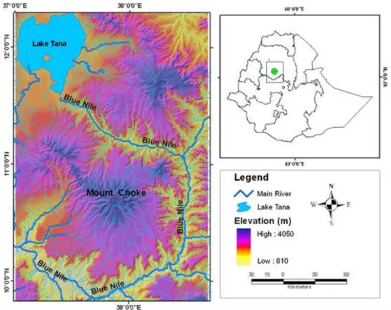
The study area covers the whole of the Choke Mountain range, the most important source of water for the Blue Nile river system in Ethiopia. The area extends between 10◦ to 11◦N and 37◦30′ to 38◦30′E, the highest peak is lo-cated at 10◦42′N and 37◦50′E. It is situated in the south of Lake Tana, in the central part of the Amhara National State of Ethiopia (Fig. 1). Elevation extends from 810 m a.s.l. to 4050 m a.s.l. The mean annual rainfall varies between 995 mm a−1 and 1864 mm a−1 based on data from 13
sta-tions for the years 1971–2006. The mean annual temperature ranges from 7.5◦C to 28◦C (BCEOM, 1998a).
The Choke Mountain is the water tower of the region serv-ing as headwater of the upper Blue Nile basin. Many of the tributaries of the Upper Blue Nile originate from this mountain range. A total of 59 rivers, and many springs are identified in the upper catchments of Choke Mountain. The Blue Nile is the largest tributary of the Nile river, the runoff being generated almost all in Ethiopia. Estimates of the mean annual flow range from 45.9×10⁹m3a−1 to
54×109m3a−1(UNESCO, 2004; Conway, 2005). The
an-nual sediment discharge of the basin at the Sudanese bor-der is between 130×106t a−1and 335
Fig. 1.The location and topography of the study area.
1998b). The major sources of sediment is erosion of the in-tensively farmed highland areas in the central and eastern parts of the basin (Bewket and Teferi, 2009; UNESCO, 2004; Zeleke, 2000).
The main geological unit in the area is the Tarmaber Gussa formation which represents Oligocene to Miocene basaltic shield volcanoes with minor trachyte and phonolite intru-sions (Tefera et al., 1999). The soil units covering the Choke Mountain are Haplic Alisols (deep soils with predominant clay or silt-clay texture), Eutric Leptosols (shallow soils with loam or clay-loam texture) and Eutric Vertisols (deep soils with clayey texture and angular/sub-angular blocky struc-ture) (BCEOM, 1998c). Due to active morphological pro-cesses (erosion, land slides etc.) the soil depth can vary be-tween zero and several meters.
There is no longer significant natural forest cover in this mountain range. The major remaining natural habitats are moisture moorland, sparsely covered with giant lobelias ( Lo-belia spp.; Jibara/Jibbra), lady’s mantle (Alchemilla spp.), Guassa grass (Festucaspp.) and other grasses. There is very little natural woody plant cover; heather (Ericaspp.; Asta) and Hypericum (Hypericum revolutum; Amijja) are found in patches. Bamboo or Kerkeha (Arundinaria alpina) is found as homestead plantation as well as part of the natural vegeta-tion cover in the area, albeit very sparsely. Korch (Erithrina brucei) is commonly grown as border demarcation plant in
the area.Eucalyptus globulusis extensively grown in planta-tion, and some of the residents have become dependent on it for their livelihoods.
3.2 Data used and image preprocessing
Table 1.Description of Landsat images used.
1986 2005
Dry Season Wet Season Dry Season Wet Season
Collection type Landsat C. Landsat C. GLS collection Landsat SLC-on
Satellite Landsat 5 Landsat 5 Landsat 7 Landsat 7
Sensor TM TM ETM+ ETM+
Path/Row 169/053 169/053 169/053 169/053
Acquisition date 28 Feb 1986 9 Nov 1985 24 Nov 2005 15 Oct 2002
Pixel spacing (m) 28.5 28.5 30 30
Sun Elevation 44.52 50.425 50.7467 58.87
Sun Azimuth 128.79 132.73 141.585 125.86
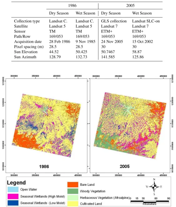
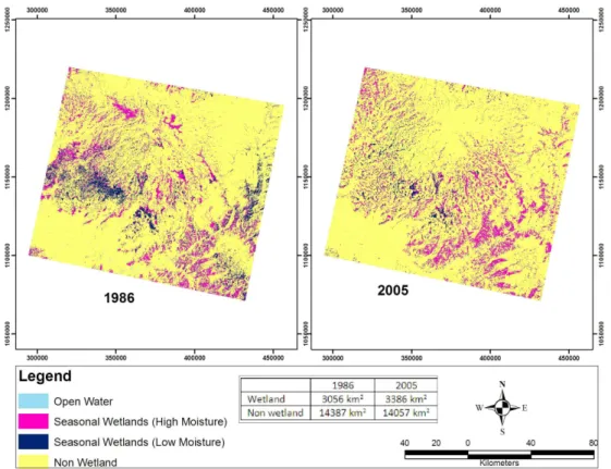
Fig. 2.Land covers in 1986 and 2005.
Sixteen-day Moderate Resolution Imaging Spectrora-diometer (MODIS) derived Normalized Difference Vegeta-tion Index (NDVI) at a resoluVegeta-tion of 250 m gained from USGS, Land Processes Distributed Active Archive Cen-ter, Moderate Resolution Imaging Spectroradiometer (USGS Land DAAC MODIS version 005 EAF NDVI) to character-ize the final wetland classes.
Several preprocessing methods were implemented before the classification and the change detection. These include ge-ometric correction, radige-ometric correction, atmospheric cor-rection, topographic normalization and temporal normaliza-tion. The importance of each preprocessing steps has been
discussed extensively in the literature (e.g., Hill and Sturm, 1991; Han et al., 2007; Vicente-Serrano et al., 2008). The specific preprocessing steps followed in this research are briefly described below.
3.2.1 Geometric correction
SPOT-5 imagery. The misaligned scenes were georectified to the underlying base layers by using control points.
In this study, first the GLS 2005 Landsat 7 ETM+ was ge-ometrically rectified using 25 control points taken from the topographic map at 1:50 000 and 11 GPS points taken in the field. The other images were then registered to the ETM+ image with the same projection. An RMS error of less than 0.5 was achieved. The nearest neighbor resampling method was used to avoid altering the original pixel values of the im-age data. Because of the high incidence of varied topography in the study area, ortho-correction was found to be necessary and hence undertaken to further enhance the image geometry by accounting for the significant spatial distortion caused by relief displacement.
3.2.2 Radiometric calibration
The absolute radiometric correction method used in this pa-per involved a combination of cross-calibration method de-veloped by Vogelman et al. (2001), with an atmospheric cor-rection algorithm based on COST model (Chavez, 1996), de-noted DOS3 by Song et al. (2001). Paolini et al. (2006) called this combination of methods “Vogelman-DOS3”.
Cross-calibration
When using both Landsat TM and ETM+ images in studies that require radiometric consistency between images, special attention has to be paid to the differences in sensors response. Previous studies have demonstrated significant differences in the radiometric response between Landsat ETM+ and Land-sat TM spectral bands (Teillet et al., 2001; Vogelmann et al., 2001). To reduce these differences and ensure image inter-comparability, a cross-calibration was needed (Paolini et al., 2006; Vicente-Serrano et al., 2008). In the cross-calibration procedure, the Landsat TM images DN (DN5) were first con-verted to the Landsat ETM+ DN (DN7) images using the equation developed by Vogelmann et al. (2001). After this conversion, the L5 TM DN is treated as L7 ETM+ DN, and L7 ETM+ gain, offset and ESUN values are used respectively for radiance and Top-Of-Atmosphere (TOA) reflectance. Conversion to at-sensor spectral radiance
At-sensor spectral radiance was computed for the cross-calibrated Landsat 5-TM (1986 images) quantized cross-calibrated pixel values in DNs and Landsat 7-ETM+ quantized cali-brated pixel values in DNs using sensor calibration param-eters published by Chander et al. (2009) and in image header file.
3.2.3 Conversion to Top of Atmosphere (TOA) reflectance
To correct for illumination variations (sun angle and Earth-Sun distance) within and between scenes, TOA reflectance
for each band was calculated. This conversion is a very important step in the calculation of an accurate Normalized Difference Vegetation Index (NDVI) and other vegetation in-dices. Some of the parameters for the conversion are avail-able in the image header files, while the exo-atmospheric ir-radiance values for Landsat 7 are published by Chander et al. (2009).
3.2.4 Atmospheric correction
TOA reflectance value does not take into account the sig-nal attenuation by the atmosphere, which strongly affects the intercomparability of the satellite images taken on dif-ferent dates. But atmospheric correction methods account for one or more of the distorting effects of the atmosphere and thereby convert the brightness values of each pixel to ac-tual reflectances as they would have been measured on the ground.
Several atmospheric correction models have been devel-oped to eliminate atmospheric effects to retrieve correct physical parameters of the earth’s surface (e.g. Surface re-flectance), including SMAC (Rahman and Dedieu, 1994), 6S (Vermote et al., 1997), MODTRAN (Berk et al., 1999), ATCOR (Richter, 1996), and COST (Chavez, 1996). De-spite the variety of available techniques, a fully image-based technique developed by Chavez (1996) known as the COST model that derives its input parameters from the image itself, has been proved to provide a reasonable atmospheric correc-tion (Mahiny and Turner, 2007; Berberoglu and Akin, 2009). The COST atmospheric model was used to convert the at-sensor spectral radiance to reflectance at the surface of the Earth.
3.2.5 Topographic correction
In mountainous regions such as Upper Blue Nile Basin, to-pographic effects that result from the differences in illumina-tion due to the angle of the sun and the angle of terrain pro-duce different reflectances for the same cover type. Hence, the classification process for rugged terrain is seriously af-fected by topography and needs careful treatment of the data (Hodgson and Shelley, 1994; Hale and Rock, 2003).
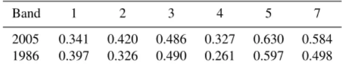
Table 2. C-correction coefficients derived for the non-Lambertian corrected images.
Band 1 2 3 4 5 7
2005 0.341 0.420 0.486 0.327 0.630 0.584
1986 0.397 0.326 0.490 0.261 0.597 0.498
model (DEM), and sun orientation information was gathered from image header data. The Regress module in IDRISI cal-culated the C-correction coefficient by regressing actual ra-diance values of each image band (the dependent variable) and cosine of the incident solar angle (the independent vari-able). The derived C-correction coefficients (Table 2) were then used as parameters to normalize both images for topo-graphic effects.
Besides visual analysis, the evaluation of topographic cor-rection was based on the computation ofR2-values for the
linear regression between corrected data and cosine of the in-cident solar angle. Since the topographic impact varies with wavelength and is most prevalent in the near-infrared spec-tral region, a reduction in theR2-value for the near-infrared
band was observed (0.214 to 0.008 for the 1986 image and 0.291 to 0.0342 for the 2005 image). This indicates the ef-fectiveness of the non-Lambertian C-correction.
3.2.6 Temporal normalization
Vicente-Serrano et al. (2008) recommended an additional step (temporal normalization) to completely remove non-surface noise and improve temporal homogeneity of satel-lite imagery. Therefore 9 reservoir sites and 5 bare sites were used to normalize the 2005 ETM+ image (slave) with respect to 1986 TM image (reference). The resulting normalization equation is shown in Table 3.
3.2.7 Image classification
A hybrid supervised/unsupervised classification approach was used to classify the images. This approach involved: (1) unsupervised classification using ISODATA (Iterative Self-Organizing Data Analysis) to determine the spectral classes into which the image resolved; (2) using the spec-tral clusters ground truth (reference data) were collected to associate the spectral classes with the cover types observed at the ground for the 2005 image and for the 1986 image reference data were collected from the 1984 Topographic map (1:50 000 scale); and (3) classification of the entire im-age using the maximum likelihood algorithm. A hierarchical class grouping was adopted to label and identify the classes (Thenkabail et al., 2005) in both the wet and dry season im-ages. First, the unsupervised ISODATA clustering was used. 25 initial classes were found and then after a rigorous iden-tification and labeling process the original 25 classes were
progressively reduced to 17, 7 and 4 classes by using ground truth data. Ground truth data on spatial location, land cover types, soil moisture status, and topographic characteristics were collected from selected sample sites during the period from June 2009 to March 2010. Stratified random sampling design was adopted for the selection of 342 point sample sites. Stratification was based on the accessibility of the sites. Spatial locations were obtained using a GPS (Global Posi-tioning System).
To assist within class identification process in the unsuper-vised classes, the at-sensor reflectance based NDVI (Normal-ized Difference Vegetation Index) values were calculated. Wetlands with covers of barren lands and/or with sparse veg-etation have lower NDVI values as a result of soil moisture that is relatively higher than the surrounding areas. When wetlands have vegetation or crops the NDVI will vary de-pending on vegetation density and vigor.
At-sensor reflectance based Tasseled Cap wetness values (Huang et al., 2002) were also calculated for both Landsat ETM+ (2005) and cross-calibrated TM (1986) images us-ing the Raster Calculator in ArcGIS 9.3. Tasseled Cap co-efficients of 0.2626 (B1), 0.2141 (B2), 0.0926 (B3), 0.0656 (B4),−0.7629 (B5), and−0.5388 (B7) were used. The Den-sity Slice tool in the ENVI 4.5 software was used to select data ranges and colors for highlighting wetland/non-wetland areas from the spectral classes.
3.2.8 Post-classification processing and assessment
A variety of change detection techniques have been devel-oped (Yuan et al., 1998; Lu et al., 2004). Each of them has its own merit and no single approach is optimal and applicable to all cases. Yuan et al. (1998) divide the methods for change detection and classification into pre-classification and post-classification techniques. In this paper post-classification comparison change detection approach which compares two independently produced classified land use/cover maps from images of two different dates (Jensen, 2005) was used. Other studies (Mas, 1999; Civco et al., 2002) demonstrated that it was the most accurate measure of change. The princi-pal advantage of post-classification is that the two dates of imagery are separately classified; hence it does not require data normalization between two dates (e.g. Singh, 1989). The other advantage of post-classification is to provide in-formation about the nature of change (including trajectories of change) (Song et al., 2001; Coppin et al., 2004).
Table 3.Image normalization regression models developed for Choke area image.
Regression models r2 Normalization targets
1986 TM B2 =−25.2 + 1.03 (2005 ETM+ B2) 0.981 8 wet and 4 dry
1986 TM B3 =−26.4 + 1.03 (2005 ETM+ B3) 0.993 9 wet and 5 dry
1986 TM B4 =−21.7 + 0.98 (2005 ETM+ B4) 0.987 8 wet and 5 dry
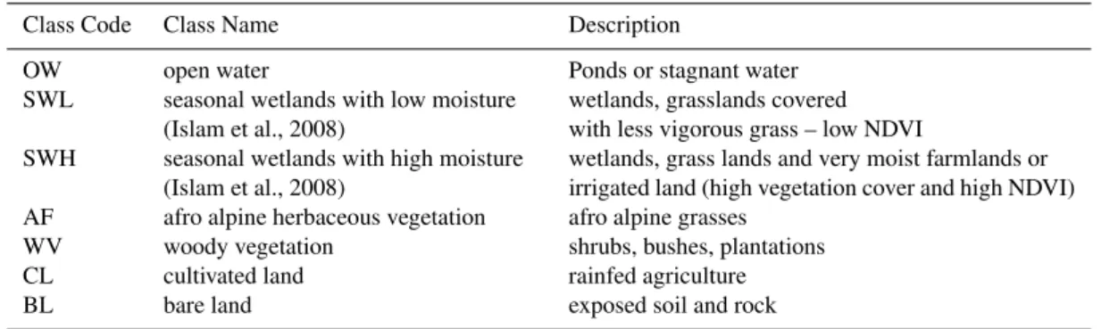
Table 4.Descriptions of the land cover classes identified in the Mt. Choke range.
Class Code Class Name Description
OW open water Ponds or stagnant water
SWL seasonal wetlands with low moisture
(Islam et al., 2008)
wetlands, grasslands covered with less vigorous grass – low NDVI
SWH seasonal wetlands with high moisture
(Islam et al., 2008)
wetlands, grass lands and very moist farmlands or irrigated land (high vegetation cover and high NDVI)
AF afro alpine herbaceous vegetation afro alpine grasses
WV woody vegetation shrubs, bushes, plantations
CL cultivated land rainfed agriculture
BL bare land exposed soil and rock
class. Finally, a detailed tabulation of changes in wetland and non-wetland classes between 1986 and 2005 classifica-tion images were compiled by post-classificaclassifica-tion comparison
4 Results and discussion
The study area was classified into seven classes: three wet-land classes and four non-wetwet-land classes. The description for each class is given in Table 4. Although riparian vegeta-tion cover defines one type of wetland, because of the lim-itation of the classification method used it was classified as woody vegetation.
A Confusion Matrix was computed to assess the accuracy of the classification by comparing the classification results with ground truth information. From the Confusion Matrix report 94.1% and 93.5% overall accuracy for the 1986 and 2005 imageries were attained, respectively. The overall ac-curacy was calculated by summing the number of pixels clas-sified correctly and dividing by the total number of pixels. An overall accuracy level of 85% was adopted as represent-ing the cutoff point between acceptable and unacceptable re-sults according to Anderson et al. (1976). The Confusion Matrix also reports the Kappa Coefficient (k) which is
an-other measure of the accuracy of the classification (Cohen, 1960). Thek values for the 1986 and 2005 image
classifi-cation were 0.908 and 0.913, respectively. The values can range from−1 to +1. However, since there should be a
pos-itive correlation between the remotely sensed classification and the reference data, positivekvalues indicate the
good-ness of the classification. Landis and Koch (1977)
character-ized the possible ranges fork into three groupings: a value
greater than 0.80 (i.e., 80%) represents strong agreement; a value between 0.40 and 0.80 (i.e., 40–80%) represents mod-erate agreement; and a value below 0.40 (i.e., 40%) repre-sents poor agreement.
The accuracies for both the 1986 and 2005 image clas-sification were considered good enough to apply post-classification change detection analysis. Basically this anal-ysis focuses on the initial state classification changes (1986 image). For each initial state class (1986), the post-classification comparison technique identifies the classes into which those pixels changed in the final state image (2005).
4.1 Space-time dynamics of non-wetland land cover types
Table 5.Change detection statistics.
Initial State Image (1986)
OW SWH SWL AF WV CL BL Class Total
OW 15.4 25.0 0.5 0.0 0.0 0.1 5.4 46.4
Final
State
Image
(2005) SWH 27.3 748.7 275.3 52.2 122.9 1621.7 151.5 2999.6
SWL 0.0 132.3 111.5 15.1 10.9 64.0 5.7 339.5
AF 0.0 96.0 13.7 79.9 49.9 47.3 12.4 299.2
WV 17.0 301.4 59.3 34.1 328.7 1351.0 873.2 2964.7
CL 6.9 632.8 422.0 38.3 307.2 6687.3 674.3 8768.8
BL 2.2 104.7 64.0 7.6 71.2 1002.7 772.1 2024.5
Class Total 68.8 2040.9 946.3 227.2 890.8 10774.1 2494.6
OW=open water, SWH=seasonal wetlands with high moisture, SWL=seasonal wetlands with low moisture, AF=afro alpine herbaceous vegetation, WV=woody vegetation, CL=cultivated land, BL=bare land
cultivated land and 30% (873.2 km2) from bare land cate-gories. Since the productive capacity of the the cultivated land is being threatened by the loss of nutrients through ero-sion, farmers in the area are looking for another option be-cause they could not cope with declining crop yields. Ev-ery year more and more agricultural land is being converted into Eucalyptus forest plantation which ensures income se-curity for local residents. This trend in use and land-cover change is altering the soil (Bewket and Stroosnijder, 2003) and hydrologic (Bewket and Sterk, 2005) characteris-tics of upland watersheds of the Choke Mountain range. This may also influence the livelihoods of the population living in downstream areas by changing critical watershed functions (e.g. availability of water during the dry season).
4.2 Space-time dynamics of wetlands
In the initial state (1986) image, 946.3 km2 of land was classified as seasonal wetlands with low moisture, but only 339.5 km2of land was classified as seasonal wetlands with low moisture in the final state image. This means a total of 607 km2 of seasonal wetlands with low moisture were lost and/or converted to another land cover/use type during the period 1986 to 2005 (Table 5). Out of the 946.3 km2of sea-sonal wetlands with low moisture class in the initial state im-age, only 111.5 km2(12%) remain unchanged and 835 km2 (88%) of the initial class has been converted and this makes the class most dynamic (unstable) of all observed land cover types. About 422 km2(∼51%), 275.3 km2(∼33%), 64 km2
(8%), and 59.3 km2(7%) of the previous seasonal wetlands with low moisture cover were converted to cultivated land, seasonal wetland with high moisture, bare land, and woody vegetation respectively. Every year 21 km2of seasonal wet-lands with low moisture land cover types are converted to cultivated land. This indicates that the experience of wetland cultivation which is common in south-wet Ethiopia (Dixon and Wood, 2003; Dixon, 2002) is also practiced in Choke Mountain range. With the increase in population pressure
Fig. 3.Proportions of land cover types in 1986 and 2005.
and shortage of land, government considers wetland culti-vation as a remedy to address the food needs (Wood, 1996; World Bank, 2001). As a result, seasonal wetlands with low moisture have come under pressure.
Fig. 4.Spatial distribution of wetland and non wetland.
wetland) in the 1990s. Jedeb irrigation project located at Yewla village (East Gojam) constructed in 1996 by diverting Jedeb river through a diversion weir (11◦22′N and 37◦33′E) is one of the best examples.
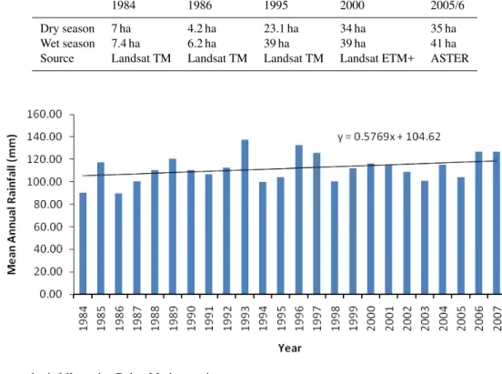
In the initial state (1986) image, 68.8 km2 of land was classified as open water and 46.4 km2 of land was classi-fied as open water in the final state image. This means a total of 22.4 km2of open water wetlands were lost and con-verted to another land cover/use type during the period 1986 to 2005. About 40% (27.3 km2) of the initial open water class were converted to seasonal wetlands with high mois-ture, 25% (17 km2) to bare land and 22% (15.4 km2) remain unchanged. According to farmers of the locality Wezem pond and Ginchira pond located in Muga watershed of Choke Mountain are now being converted to bare land. This was also substantiated by field observation. In contrast, Bahir-dar pond (Fig. 5) at Yenebirna village in Chemoga water-shed showed a gradual increase through time (Table 6). To analyze this situation 10 satellite images (5 on dry season and 5 on wet season) were taken and the size of Bahirdar pond was determined. The observed smallest size (4.2 ha) could be because of the 1986 drought occurred throughout Ethiopia. This indicated that the condition of wetlands of the area is dependent on climatic factors beyond human in-fluences. The increasing trend of rainfall of the area around the pond (Fig. 6) associated with increasing runoff and sedi-ment inflow from the surrounding watershed could be one of
Fig. 5.Open water wetland at Yenebrna village (East Gojam).
the reasons for the gradual increase of the pond. A study by McHugh et al. (2007) explained one example from north-east Ethiopia for the case of Hara swamp.
4.3 Characterization of wetlands
Table 6.Time-series of pond size.
1984 1986 1995 2000 2005/6
Dry season 7 ha 4.2 ha 23.1 ha 34 ha 35 ha
Wet season 7.4 ha 6.2 ha 39 ha 39 ha 41 ha
Source Landsat TM Landsat TM Landsat TM Landsat ETM+ ASTER
Fig. 6.The mean annual rainfall trend at Debre Markos station.
16-day Normalized Difference Vegetation Index (NDVI) at a resolution of 250 m gained from United States Geological Survey, Land Processes Distributed Active Archive Center.
Deep open water shows lower NDVI values than the other wetland classes throughout the year. Because open water fea-tures have lower near infrared reflectance. The standard de-viation of the response of open water to NDVI is the least (0.06) among the 7 land cover lasses. Indicating that a more or less constant response to NDVI except during rainy sea-son. The increase in runoff with increase in trapped sediment during rainy season may change the normal NDVI response. The highest variance (0.18) is observed in seasonal wetland with high moisture land cover classes. These classes show higher NDVI values in September and lower values during the period 22 March to 6 April. Seasonal wetlands with high moisture and low moisture classes are clearly distinct during the period from end of August to December.
The NDVI time-series class characteristics follows the rainfall trend (Fig. 7); vegetation begins to gain vigor in be-ginning of September and remains at high vigor until Novem-ber while the rainfall reaches maximum during 28 July to 12 August. Previous studies have investigated the lag and cumu-lative effect of rainfall on vegetation in semi-arid and arid re-gions of Africa (Martiny et al., 2006; Wagenseil and Samimi, 2006) and humid regions of Africa (Onema and Taigbenu, 2009). However, this lag effect of rainfall can not be ob-served in open water.
5 Conclusions
The study demonstrated the use of remote sensing techniques to delineate headwater wetlands from non-wetlands and de-termine the dynamics over large areas of Choke Mountains with the overall accuracy of 94.1% and 93.5% and Kappa Coefficient of 0.908 and 0.913 for the 1986 and 2005 im-ageries, respectively. Therefore, ground-based wetland sur-veying for large area, especially for small wetlands is a very time consuming and ineffective process. The use of Remote Sensing and GIS techniques in wetland mapping reduces cost and enhances the accuracy. Creating radiometrically consis-tent image data through (Vogelman-DOS3) methods before applying hybrid supervised/unsupervised classification was found to be effective in wetland mapping. However the ap-plication of technique to Landsat images was not effective in mapping riparian vegetation as wetland. To undertake a more focused wetland management plan implementation the use of mandatory environmental characteristics (vegetation, soil, and hydrology) for wetland detection is still important.
Four major trajectories of change that were observed: (1) from seasonal wetlands with low moisture to cultivated land, (2) from cultivated land to woody vegetation (planta-tion), (3) from open water to bare land, and (4) from bare land to cultivated land. In general, 607 km2of seasonal wet-land with low moisture and 22.4 km2of open water are lost
in the study area over the 20 years considered. This is one indication of future deterioration in wetland condition. This calls for wetland conservation and rehabilitation through in-corporating wetlands into watershed management plans so as to make wetlands continue providing their multiple func-tions which include flood control, stream-flow moderation, groundwater recharge, sediment detention, and pollutant re-tention. Further research on specific wetland spots is needed for accurate inventories of wetlands and to explore the rea-sons why and how wetlands are changing.
Acknowledgements. The study was carried out as a project within a larger research program called “In search of sustainable catchments and basin-wide solidarities in the Blue Nile River Basin”, which is funded by the Foundation for the Advancement of Tropical Research (WOTRO) of the Netherlands Organization for Scientific Research (NWO), UNESCO-IHE and Addis Ababa University. The authors are grateful to US Geological Survey (USGS) Center for Earth Resources Observation and Science (EROS) and Land Processes Distributed Active Archive Center (Land DAAC) for providing research data free of charge.
Edited by: A. Melesse
References
Anderson, J. R., Hardy, E. E., Roach, J. T., and Witmer, R. E.: A land use and land cover classification system for use with re-mote sensor data, USGS Professional Paper 964, Sioux Falls, SD, USA, 1976.
Baker, C., Lawrence, R., Montagne, C., and Patten, D.: Mapping wetlands and riparian areas using Landsat ETM+ imagery and decision-tree-based models, Wetlands, 26, 465–474, 2006. BCEOM: Abbay River Basin Integrated Development Master
Plan-Phase 2 – Water Resources – Climatology, Ministry of Water Resources, Addis Ababa, 144 pp., 1998a.
BCEOM: Abbay River Basin Integrated Development Master Plan-Phase 2 – Water Resources – Hydrology, Ministry of Water Re-sources, Addis Ababa, 144 pp., 1998b.
BCEOM: Abbay River Basin Integrated Development Master Plan-Phase 2 – Land Resources Development – Reconnaissance Soils Survey, Ministry of Water Resources, Addis Ababa, 208 pp., 1998c.
Berberoglu, S. and Akin, A.: Assessing different remote sens-ing techniques to detect land use/cover changes in the eastern Mediterranean, Int. J. Appl. Earth Obs., 11, 46–53, 2009. Berk, A., Anderson, G. P., Bernstein, L. S., Acharya, P. K., Dothe,
H., Matthew, M. W., Adler-Golden, S. M., Chetwynd, J. H., Richtsmeier, S. C., Pukall, B., Allred, C. L., Jeong, L. S., and Hoke, M. L.: MODTRAN4 radiative transfer modeling for at-mospheric correction, in: Proceedings of SPIE Optical Spec-troscopic Techniques and Instrumentation for Atmospheric and Space Research III, Denver, Co, USA, 18 July 1999, 1999. Bewket, W.: Household level tree planting and its implications for
Bewket, W. and Sterk, G.: Dynamics in land cover and its ef-fect on stream flow in the Chemoga watershed, Blue Nile basin, Ethiopia, Hydrol. Process., 19, 445–458, 2005.
Bewket, W. and Stroosnijder, L.: Effects of agro-ecological land use succession on soil properties in Chemoga watershed, Blue Nile basin, Ethiopia, Geoderma, 111, 85–98, 2003.
Bewket, W. and Teferi, E.: Assessment of Soil Erosion Hazard and Prioritization for Treatment at the Watershed Level: Case Study in the Chemoga Watershed, Blue Nile Basin, Ethiopia, Land De-grad. Dev., 20, 609–622, 2009.
Callan, O. and Mark, A. F.: Using MODIS data to characterize seasonal inundation patterns in the Florida Everglades, Remote Sens. Environ., 112, 4107–4119, 2008.
Civco, D. L., Hurd, J. D., Wilson, E. H., Song, M., and Zhang, Z.: A Comparison of Land Use and Land Cover Change Detection Methods, in: Proceedings of 2002 ASPRS-ACSM Annual Con-ference and FIG XXII Congress, Washington, D.C., 22–26 April 2002, 12 pp., 2002.
Chander, G., Markham, B. L., and Helder, D. L.: Summary of cur-rent radiometric calibration coefficients for Landsat MSS, TM, ETM+, and EO-1 ALI sensors, Remote Sens. Environ., 113, 893–903, 2009.
Chavez, P. S.: Image-based atmospheric corrections-revisited and improved, Photogramm. Eng. Rem. S., 62, 1025–1036, 1996. Cohen, J.: A coefficient of agreement for nominal scales, Educ.
Psychol. Meas., 20, 37–40, 1960.
Colby, J. D.: Topographic normalization in rugged terrain, Pho-togramm. Eng. Rem. S., 62, 151–161, 1991.
Conway, D.: From headwater tributaries to international river: Ob-serving and adapting to climate variability and change in the Nile Basin, Global Environmental Change, 15, 99–114, 2005. Coppin, P., Jonckheere, I., Nackaerts, K., Muys, B., and Lambin,
E.: Digital change detection methods in ecosystem monitoring: A review, Int. J. Remote Sens., 25, 1565–1596, 2004.
Dixon, A. B.: The hydrological impacts and sustainability of wet-land drainage cultivation in Illubabor, Ethiopia, Land Degrad. Dev., 13, 17–31, 2002.
Dixon, A. B. and Wood, A. P.: Wetland cultivation and hydrologi-cal management in eastern Africa: Matching community and hy-drological needs through sustainable wetland use, Nat. Resour. Forum, 27, 117–129, 2003.
Ehrenfeld, J. G.: Evaluating wetlands within an urban context, Ecol. Eng., 15, 253–265, 2000.
Finlayson, C. M., Davidson, N. C., Spiers, A. G., and Stevenson, N. J.: Global wetland inventory – current status and future priorities, Mar. Freshwater Res., 50, 717–727, 1999.
Frazier, S. P. and Page, J. K.: Water body detection and delineation with Landsat TM data, Photogramm. Eng. Rem. S., 66, 1461– 1467, 2000.
Hadjimitsis, D. G., Clayton, C. R. I., and Hope, V. S.: An assess-ment of the effectiveness of atmospheric correction algorithms through the remote sensing of some reservoirs, Int. J. Remote Sens., 25, 3651–3674, 2004.
Hailu, A., Wood, A. P., and Dixon, A. B.: Interest groups, local knowledge and community management of wetland agriculture in South-West Ethiopia, Int. J. Ecol. Environ. Sci., 29, 55–63, 2003.
Hale, S. R. and Rock, B. N.: Impact of Topographic Normaliza-tion on Land-Cover ClassificaNormaliza-tion Accuracy, Photogramm. Eng.
Rem. S., 69(7), 785–791, 2003.
Han, T., Wulder, M. A., White, J. C., Coops, N. C., Alvarez, M. F., and Butson, C.: An efficient protocol to process Landsat images for change detection with tasselled cap transformation, IEEE Geosci. Remote S., 4, 147–151, 2007.
Hill, J. and Sturm, B.: Radiometric correction of muli-temporal Thematic Mapper data for use in agricultural land-cover classi-fication and vegetation monitoring, Int. J. Remote Sens., 12(7), 1471–1491, 1991.
Hodgson, M. E. and Shelley, B. M.: Removing the topographic ef-fect in remotely sensed imagery, ERDAS Monitor, 6, 4–6, 1994. Holben, B. N. and Justice, C. O.: The topographic effect on spectral response from nadir-pointing sensors, Photogramm. Eng. Rem. S., 46, 1191–1200, 1980.
Huang, C., Wylie, B., Yang, L., Homer, C., and Zylstra, G.: Deriva-tion of a Tassled Cap transformaDeriva-tion based on Landsat and at-satellite reflectance, Int. J. Remote Sens., 23, 1741–1748, 2002. Islam, Md. A., Thenkabail, P. S., Kulawardhana, R. W., Alankara,
R., Gunasinghe, S., Edussriya, C., and Gunawardana, A.: Semi-automated methods for mapping wetlands using Landsat ETM+ and SRTM data, Int. J. Remote Sens., 29, 7077–7106, 2008. Jensen, J. R.: Introductory digital image processing: A remote
sens-ing perspective, 3rd Edn., Prentice Hall, Upper Saddle River, NY, 526 pp., 2005.
Jensen, J. R., Narumalani, S., Weatherbee, O., and Mackey, H.
E.: Measurement of Seasonal and Yearly Cattail and
Wa-terlily Changes Using Multidate SPOT Panchromatic Data, Pho-togramm. Eng. Remote S., 59, 519–525, 1993.
Koeln, G.: How wet is this wetland? Earth Observation Magazine, July/August, 36–39, 1992.
Landis, J. and Koch, G.: The measurement of observer agreement for categorical data, Biometrics, 33, 159–174, 1977.
Lemma, B.: Human intervention in two lakes: Lessons from Lakes Alemaya and Hora-Kilole, in: Proceedings of the National Con-sultative workshop on the Ramsar Convention and Ethiopia, 18– 19 March 2004, Addis Ababa, Ethiopia, 2004.
Loiselle, S., C´ozar, A., van Dam, A. A., Kansiime, F., Kelderman, P., Saunders, M., and Simonit, S.: Development of tools for wet-land ecosystem resource management in East Africa, in: Wet-lands and Natural Resource Management: Ecological Studies, edited by: Verhoeven, J. T. A., Beltman, B., Bobbink, R., and Whigham, D. F., Springer, Berlin, 97–122, 2006.
Lu, D., Mausel, P., Brondizio, E., and Moran, E.: Change Detection Techniques, Int. J. Remote Sens., 25, 2365–2407, 2004. Mac, M. J., Opler, P. A., Puckett Haecker, C. E., and Doran, P.
D.: Status and trends of the nation’s biological resources, 2 vol., US Department of the Interior, US Geological Survey, Reston, Va., 1998, http://www.nwrc.usgs.gov/sandt/index.html, last ac-cess: 24 June 2010.
Mahiny, A. S. and Turner, B. J.: A comparison of four common atmospheric correction methods, Photogramm. Eng. Rem. S., 73, 361–368, 2007.
Markham, B. L. and Barker, J. L.: Landsat MSS and TM post-calibration dynamic ranges, exoatmospheric reflectances and at-satellite temperatures, EOSAT Landsat Technical Notes, 1, 3–8, 1986.
Mas, J. F.: Monitoring land-cover changes: a comparison of change detection techniques, Int. J. Remote Sens., 20, 139–152, 1999. Matthews, E. and Fung, I.: Methane emissions from natural
wet-lands: global distribution, area, and environmental characteris-tics of sources, Global Biogeochem. Cy., 1, 61–86, 1987. McDonald, E. R., Wu, X., Caccetta, P. A., and Campbell, N. A.:
Il-lumination Correction of Landsat TM Data in South East NSW, in: Proceedings of the Tenth Australasian Remote Sensing and Photogrammetry Conference, Adelaide, Australia, 21–25 Au-gust, 2000.
McHugh, O. V., McHugh, A. N., Eloundou-Enyegue, P. M., and Steenhuis, T. S.: Integrated Qualitative Assessment of Wetland Hydrological and Land Cover Changes in a Data Scarce Dry Ethiopian Highland Watershed, Land Degrad. Dev., 18, 643–658, 2007.
McKergow, L. A., Gallant, J. C., and Dowling, T. I.: Modelling wet-land extent using terrain indices, Lake Taupo, NZ, in: Proceed-ings of MODSIM 2007 International Congress on Modelling and Simulation, Modelling and Simulation Society of Australia and New Zealand, December 2007, 74–80, 2007.
Meyer, P., Itten, K., Kellenberger, T., Sandmeier, S., and Sandmeier, R.: Radiometric corrections of topographically induced effects on Landsat TM data in an alpine environment, ISPRS J. Pho-togramm., 48(4), 17–28, 1993.
Mohamed, Y. A., van den Hurk, B. J. J. M., Savenije, H. H. G., and Bastiaanssen, W. G. M.: Hydroclimatology of the Nile: results from a regional climate model, Hydrol. Earth Syst. Sci., 9, 263– 278, doi:10.5194/hess-9-263-2005, 2005.
Moser, M., Prentice, C., and Frazier, S.: A global overview of wet-land loss and degradation, in: Proceedings of the 6th Meeting of the Conference of Contracting Parties of the Ramsar Convension, Brisbane, Australia, 19–27 March 1996, 21–31, 1996.
Mulugeta, M.: Socio-economic Determinants of Wetland use in the Metu and Yayu-Hurumu Weredas of Illubabor Zone, in: Sustain-able Management of Wetlands in Illubabor Zone, 13 December 1999, Addis Ababa, Ethiopia, 1999.
OECD: Guidelines for Aid Agencies for Improved Conservation and Sustainable Use of Tropical and Sub-Tropical Wetlands, Paris, France, OECD Guidelines on Aid and Environment, 9, 67 pp., 1996.
Onema, J. K. and Taigbenu, A.: NDVI-rainfall relationship in the Semliki watershed of the equatorial Nile, Phys. Chem. Earth, 34, 711–721, 2009.
Ozesmi, S. L. and Bauer, M. E.: Satellite remote sensing of wet-lands, Wetl. Ecol. Manag., 10, 381–402, 2002.
Pantaleoni, E., Wynne, R. H., Galbraith, J. M., and Campbell, J. B.: Mapping wetlands using ASTER data: a comparison between classification trees and logistic regression, Int. J. Remote Sens., 30, 3423–3440, 2009.
Paolini, L., Grings, F., Sobrino, J. A., Jim´enez Mu˜noz, J. C., and Karsebaum, H.: Radiometric correction effects in Landsat multi-date/multi-sensor change detection studies, Int. J. Remote Sens., 27, 685–704, 2006.
Rahman, H. and Dedieu, G.: SMAC: a simplified method for the at-mospheric correction of satellite measurements in the solar spec-trum, Int. J. Remote Sens., 15, 123–143, 1994.
Ramsar Convention Secretariat: The Ramsar Convention Manual: a guide to the Convention on Wetlands (Ramsar, Iran, 1971), 4th edn., Ramsar Convention Secretariat, Gland, Switzerland, 2006.
Reimold, R. J.: Wetlands functions and values, in: Applied Wet-lands Science and Technology, edited by: Kent, D. M., Lewis Publishers, Boca Raton, LA, USA, 55–78, 1994.
Ria˜no, D., Chuvieco, E., Salas, J., and Aguado, I.: Assessment of Different Topographic Corrections in Landsat-TM Data for Map-ping Vegetation Types, IEEE T. Geosci. Remote, 41, 1056–1061, 2003.
Richter, R.: A spatially adaptive fast atmospheric correction algo-rithm, Int. J. Remote Sens., 17, 1201–1214, 1996.
Schroeder, T. A., Cohen, W. B., Song, C., Canty, M. J., and Yang, Z.: Radiometric correction of multi-temporal Landsat data for characterization of early successional forest patterns in western Oregon, Remote Sens. Environ., 103, 16–26, 2006.
Singh, A.: Digital change detection techniques using remotely sensed data, Int. J. Remote Sens., 10, 989–1003, 1989.
Smith, L., Lin, T., and Ranson, K.: The Lambertian assumption and Landsat data, Photogramm. Eng. Rem. S., 46, 1183–1189, 1980. Song, C., Woodcock, C. E., Seto, K. C., Lenney, M. P., and Ma-comber, S. A.: Classification and change detection using Landsat TM data: When and how to correct atmospheric effects?, Remote Sens. Environ., 75, 230–244, 2001.
Tefera, M., Cherinet, T., and Haro, W.: Explanation of the Geo-logical Map of Ethiopia, 2nd Edn., Bulletin No. 3, EIGS, Addis Ababa, Ethiopia, 79 pp., 1999.
Teillet, P. M., Guindon, B., and Goodenough, D. G.: On the slope-aspect correction of multispectral scanner data, Can. J. Remote Sens., 8, 84–106, 1982.
Teillet, P. M., Barker, J., Markham, B. L., Irish, R. R., Fedose-jevs, G., and Storey, J. C.: Radiometric cross-calibration of the Landsat-7 ETM+ and Landsat-5 TM sensors based on tandem data sets, Remote Sens. Environ., 78, 39–54, 2001.
Thenkabail, P., Schull, M., and Turral, H.: Ganges and Indus river basin land use/land cover (LULC) and irrigated area mapping us-ing continuous streams of MODIS data, Remote Sens. Environ., 95, 317–341, 2005.
Tiner, R. W.: Geographically isolated wetlands of the United States, Wetlands, 23, 494–516, 2003.
T¨oyr¨a, J. and Pietroniro, A.: Towards operational monitoring of a northern wetland using geomatics based techniques, Remote Sens. Environ., 97, 174–191, 2005.
UNESCO: National Water Development Report for Ethiopia, UN-WATER/WWAP/2006/7, World Water Assessment Program, Re-port, MOWR, Addis Ababa, Ethiopia, 273 pp., 2004.
Van Dam, A. A., Dardona, A., Kelderman, P., and Kansiime, F.: A simulation model for nitrogen retention in a papyrus wetland near Lake Victoria, Uganda (East Africa), Wetl. Ecol. Manag.,15, 469–480, 2007.
Vermote, E. F., Tanr´e, D., Deuz´e, J. L., Herman, M., and Morcrette, J. J.: Second simulation of the satellite signal in the solar spec-trum, 6S: an overview, IEEE T. Geosci. Remote, 35, 675–686, 1997.
Vicente-Serrano, S. M., Perez-Cabello, F., and Lasanta, T.: Assess-ment of radiometric correction techniques in analyzing vegeta-tion variability and change using time series of Landsat images, Remote Sens. Environ., 112, 3916–3934, 2008.
characterization, Remote Sens. Environ., 78, 55–70, 2001. Wagenseil, H. and Samimi, C.: Assessing spatio-temporal
varia-tions in plant phenology using Fourier analysis on NDVI time series: results from a dry savannah environment in Namibia, Int. J. Remote Sens., 27, 3455–3471, 2006.
Wei, W., Zhang, X., Chen, X., Tang, J., and Jiang, M.: Wetland Mapping Using Subpixel Analysis and Decision Tree Classifica-tion in the Yellow River Delta Area, The InternaClassifica-tional Archives of the Photogrammetry, Remote Sensing and Spatial Information Sciences, Vol. XXXVII, Part B7, Beijing, 2008.
Wood, A. P.: Wetland drainage and management in south-west Ethiopia: Some environmental experiences of an NGO, in: The Sahel Workshop 1996, edited by: Reenburg, A., Marcusen, H. S., and Nielsen, I., Institute of Geography, University of Copen-hagen, CopenCopen-hagen, 1996.
Wood, A. P.: Policy implications for wetland management, in: Pro-ceedings of the National Workshop on Sustainable Wetland Man-agement, 13 December 1999, Addis Ababa, Ethiopia, 117–127, 2000.
Wood, A. P.: Wetlands, gender and poverty, in: Proceedings of a seminar on the resources and status of in Ethiopia’s wetlands, edited by: Yilma, D. A. and Geheb, K., Wetlands of Ethiopia, Gland, IUCN, 58–66, 2001.
World Bank: Project appraisal document for the Rwanda Rural Sector Support Programme, Report No: 21048-RW, The World Bank, Washington DC, 2001.
Yohannes, F.: Soil Erosion and Sedimentation: The Case of
Lake Alemaya, in: Proceedings of the Second Awareness Cre-ation Workshop on Wetlands in the Amhara Region, Bahirdar, Ethiopia, September, 2005.
Yuan, D., Elvidge, C. D., and Lunetta, R. S.: Survey of multispec-tral methods for land cover change analysis, in: Remote Sensing Change Detection: Environmental Monitoring Methods and Ap-plications, edited by: Lunetta, R. S. and Elvidge, C. D., Chelsea, MI: Ann Arbor Press, 21–39, 1998.