www.atmos-meas-tech.net/5/1375/2012/ doi:10.5194/amt-5-1375-2012
© Author(s) 2012. CC Attribution 3.0 License.
Measurement
Techniques
Evaluation of turbulent dissipation rate retrievals from Doppler
Cloud Radar
M. D. Shupe1, I. M. Brooks2, and G. Canut2
1University of Colorado and NOAA-Earth System Research Laboratory, Boulder, Colorado, USA 2Institute for Climate and Atmospheric Science, University of Leeds, Leeds, UK
Correspondence to:M. Shupe ([email protected])
Received: 16 December 2011 – Published in Atmos. Meas. Tech. Discuss.: 18 January 2012 Revised: 21 May 2012 – Accepted: 29 May 2012 – Published: 18 June 2012
Abstract. Turbulent dissipation rate retrievals from cloud radar Doppler velocity measurements are evaluated using independent, in situ observations in Arctic stratocumulus clouds. In situ validation data sets of dissipation rate are de-rived using sonic anemometer measurements from a tethered balloon and high frequency pressure variation observations from a research aircraft, both flown in proximity to station-ary, ground-based radars. Modest biases are found among the data sets in particularly low- or high-turbulence regimes, but in general the radar-retrieved values correspond well with the in situ measurements. Root mean square differences are typi-cally a factor of 4–6 relative to any given magnitude of dissi-pation rate. These differences are no larger than those found when comparing dissipation rates computed from tethered-balloon and meteorological tower-mounted sonic anemome-ter measurements made at spatial distances of a few hundred meters. Temporal lag analyses suggest that approximately half of the observed differences are due to spatial sampling considerations, such that the anticipated radar-based retrieval uncertainty is on the order of a factor of 2–3. Moreover, radar retrievals are clearly able to capture the vertical dissipation rate structure observed by the in situ sensors, while offer-ing substantially more information on the time variability of turbulence profiles. Together these evaluations indicate that radar-based retrievals can, at a minimum, be used to deter-mine the vertical structure of turbulence in Arctic stratocu-mulus clouds.
1 Introduction
Turbulence plays a central role in the life cycle of clouds by influencing their formation, maintenance, and dissipa-tion processes (Nicholls and Turton, 1986; Bretherton et al., 2004). Mixing associated with turbulent motions is respon-sible for entrainment (Nicholls and Turton, 1986; Stevens, 2002), which has direct bearing on the aerosols and mois-ture available to a cloud layer and thereby the cloud micro-physical composition. Vertical mixing also shapes the atmo-spheric thermodynamic structure within which a cloud exists. There are multiple sources of turbulence generation within the cloudy atmosphere, including processes, such as cloud top radiative cooling, that are driven by the clouds them-selves. In order to understand the physical processes oper-ating within clouds, the coevolution of the turbulent state, cloud properties, and thermodynamic structure must be char-acterized.
of hydrometeor-sensing Doppler radar (e.g. Brewster and Zr-nic, 1986; Kollias et al., 2001), velocity time series measure-ments from Doppler lidar (e.g. Banakh and Smalikho, 1997; O’Connor et al., 2010) and Doppler radar (e.g. Frisch and Strauch, 1976; Bouniol et al., 2003), and velocity structure functions derived from Doppler lidar (Frehlich and Cornman, 2002) and Doppler radar (Lothon et al., 2005).
To facilitate studies of cloud life cycle processes, it is ad-vantageous to employ an observing system that offers con-current perspectives on both cloud and turbulence proper-ties within an identical atmospheric volume. Short wave-length (<1 cm) cloud radars are well positioned to address this problem, as within a given atmospheric profile they con-tain information on the vertical location of clouds (Clothiaux et al., 2000), in-cloud vertical air motions and turbulence (e.g. Kollias et al., 2001; Deng and Mace, 2006), the phase of cloud particles (Shupe, 2007; Luke et al., 2010), and many microphysical properties (e.g. Comstock et al., 2007; Shupe et al., 2008a). Cloud radar Doppler spectral width measure-ments contain substantial information on turbulence; how-ever, other processes such as wind shear and the distribution of cloud particle fall speeds can also contribute significantly to broadening of the spectral width. The latter is particularly true for precipitating or mixed-phase conditions (e.g. Gos-sard et al., 1997; Shupe et al., 2004). This convolution of information within a given pulse volume complicates cloud radar spectral-width based turbulence retrievals (e.g. Kollias et al., 2001).
The focus here is, instead, on a technique to character-ize turbulence from time series measurements of cloud radar Doppler velocity in order to evaluate the skill with which the turbulent dissipation rate – the rate at which turbulent kinetic energy is dissipated by viscosity at small scales in the atmosphere – can be retrieved. In this case, the technique is specifically applied to observations of Arctic mixed-phase stratocumulus clouds that contain both cloud liquid water and precipitating ice crystals. While there are generally few op-portunities to evaluate such retrievals in Arctic environments, this study capitalizes on two experiments where independent measurements of turbulent dissipation rate were made in the vicinity of cloud radars. The ultimate aim of this study is to evaluate the ability of operational cloud radars (e.g. Kollias et al., 2007; Illingworth et al., 2007) to derive turbulence in-formation within mixed-phase cloud environments.
2 Methods
Observations used in this study were obtained during two Arctic field campaigns. One of these was the Arctic Summer Cloud Ocean Study (ASCOS, Sedlar et al., 2011), which took place in late summer of 2008 in the Arctic sea-ice pack near 87.4◦N, 8◦W. During this campaign, ground-based sensors, including cloud radar, were deployed aboard the Swedish icebreaker R/VOden to observe the atmospheric turbulent
structure. Complementary turbulence measurements were made using a tethered balloon system and an instrumented meteorological tower installed on the adjacent sea-ice. The second campaign was the Mixed-Phase Arctic Clouds Exper-iment (MPACE, Verlinde et al., 2007), which occurred in Oc-tober 2004 near the US. Department of Energy Atmospheric Radiation Measurement (ARM) program’s North Slope of Alaska (NSA) facility in Barrow, Alaska, USA. The basic experiment design consisted of flying a heavily instrumented research aircraft to measure cloud and atmosphere properties above the permanent, ground-based instrument suite at the NSA site.
2.1 Radar retrieval
Turbulent dissipation rates evaluated in this study are de-rived from identical, vertically-pointing, 35-GHz, Millime-ter Cloud Radars (MMCR, Moran et al., 1998) operated dur-ing these two experiments. In each case the “stratus” opera-tional mode is utilized, as it has been optimized for observing low-level clouds and is sensitive enough to observe most hy-drometeors in the lower troposphere (see Table 1). The fun-damental measurement of interest is the mean Doppler veloc-ity, which characterizes the reflectivity-weighted, mean mo-tion of hydrometeors within a quasi-cylindrical radar sample volume of 45-m vertical depth and 1- to 3-m radius depend-ing on cloud height. Doppler velocity measurements are only possible when hydrometeors are present within the volume and measurements are only used in the retrieval if they have a signal-to-noise ratio greater than−13 dB. The variance of the measured mean Doppler velocity in time, σvm2 , can be represented as (Lothon et al., 2005)
σvm2 =σw2+σvt2+2cov(w,vt) (1) whereσw2 andσvt2 are the variance contributions due to the vertical air motions (i.e. turbulence) and changes in the ter-minal fall speed of hydrometeors, respectively, and the final term is the covariance between vertical air motions and ter-minal fall speeds.
The retrieval applied to Arctic mixed-phase stratocumulus has been outlined in Shupe et al. (2008b) and is based on principles developed by Rogers and Tripp (1964), Bouniol et al. (2003), and O’Connor et al. (2005) for slightly different cloud regimes and radars. Briefly, it has been shown that the variance in measured mean Doppler velocity can be repre-sented as
σvm2 =
ks Z
kl
S(k)dk=3A
2 ε
2π
2/3
(L2l/3−L2s/3), (2)
where the turbulent energy spectrum isS(k)=Aε2/3k−5/3,
Ais the Kolmogorov constant which is assumed to be 0.51
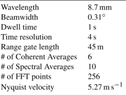
Table 1.MMCR specifications for the “stratus” operational mode.
Wavelength 8.7 mm Beamwidth 0.31◦ Dwell time 1 s Time resolution 4 s Range gate length 45 m # of Coherent Averages 6 # of Spectral Averages 10 # of FFT points 256 Nyquist velocity 5.27 m s−1
(Sreenivasan, 1995),εis the turbulent dissipation rate,kis the wave number, andLis the length scale given byL= 2π/k. Two length scales of interest areLs, which is the length of
the scattering volume for the 1-s radar dwell time includ-ing larger eddies passinclud-ing through the observation volume, andLl, which represents the larger eddies passing through
the effective sample volume that results from averaging radar observations over 60 s. Following Taylor’s frozen turbulence hypothesis (Taylor, 1935), these length scales can be related to the sampling volume geometry and the horizontal wind speed by L=U t+ 2Rsin(θ/2), where U is the horizontal wind speed,tis the sample time (1 or 60 s),Ris the range to the pulse volume, andθ is the radar beamwidth. Horizontal wind speed is interpolated to the radar time-height grid from collocated wind profiler measurements (449-MHz profiler at ASCOS, 915-MHz profiler at MPACE) with nominal 30-min time resolution; however, if wind profiler measurements are not available or inconsistent in time, winds are derived via interpolation from the nearest in time radiosoundings. Rear-ranging Eq. (2) provides a simple equation for the dissipation rate as
ε=2π
2σvm2
3AL2l/3−L2s/3
3/2
. (3)
Fundamental assumptions used to derive these equations are that the length scales of the turbulent eddies observed by the radar (i.e.Ll andLs)reside within the inertial subrange of
the turbulence spectrum and that turbulent air motions, as opposed to variability in particle terminal fall speeds due to cloud microphysical properties, are the dominant contribu-tion to variability of the mean Doppler velocity in Eq. (1) on the scales of interest.
2.2 Evaluating retrieval assumptions and uncertainty
The two primary assumptions made in this retrieval have been shown to hold for ice clouds and drizzling stratocu-mulus (Bouniol et al., 2003; O’Connor et al., 2005), both of which have some properties that are similar to mixed-phase stratocumulus. Lothon et al. (2005) used focused air-craft in situ measurements in drizzling stratocumulus to show that the variance due to hydrometeor fall speeds is an
order of magnitude smaller than the total variance of the mean Doppler velocity. Their measurements also indicate that while there is significant covariance between vertical air motions and hydrometeor fall speeds, as has also been ob-served for Arctic mixed-phase stratocumulus (Shupe et al., 2008c), the covariance acts on scales that are predominantly larger than the scales important for dissipation of turbulence. Thus, it is expected that the primary assumptions for the cur-rent retrieval will hold unless the radar is sampling eddies, via Ll, that are larger than the turbulent inertial subrange
(O’Connor et al., 2005) or if the correlation scales between vertical motions and microphysical properties become small (Lothon et al., 2005).
These assumptions will be evaluated using an example mixed-phase stratocumulus cloud that occurred on 28 Au-gust 2008 during ASCOS. A time-height plot of the radar-derived turbulent dissipation rate for this case is shown in Fig. 1c. The basic structure of the cloud consisted of a 300– 400 m thick layer of super-cooled liquid water (T ≈ −10◦C) within which ice crystals formed and then fell down towards the surface. This structure is typical of Arctic mixed-phase stratocumulus (e.g. Shupe et al., 2006). On this day there was a distinct transition in the turbulent structure at about 06:00 UTC associated with a moderate lifting of the cloud layer as weak easterly winds flowed under the otherwise northerly winds associated with the cloud layer.
The wide range of derived dissipation rates during this case allows for a nice evaluation of the basic retrieval as-sumptions; namely, that the variance in measured mean Doppler velocity is dominated by turbulence (i.e. it follows a typical Kolmogorov form with a turbulent inertial subrange having a−5/3 slope) and that the length scales sampled for the retrieval reside within the inertial subrange. Power spec-tra have been calculated via fast Fourier spec-transforms of 1011 samples (∼2 h) of radar mean Doppler velocities at a given height (Fig. 2). Time series for these analyses have been se-lected both above and below the cloud base at times before and after the transition at 06:00 UTC in order to examine a range of conditions. In each case, the high frequency end of the spectra have an approximate−5/3 slope, which is char-acteristic of the inertial subrange. Horizontal wind speeds during this case were approximately 4 m s−1, such that the largest scale sampled for the radar retrieval was 240 m. It is clear that in each case the transition from inertial subrange to outer turbulent scales occurs at scales longer than 240 m. Thus, both primary assumptions are well supported by these examples.
Fig. 1.Time-height contour maps of radar mean Doppler velocity (a), fractional error in velocity variance from Eq. (6) (b), radar-retrieved turbulent dissipation rate(c), and fractional error in re-trieved dissipation rate from Eq. (7)(d)for a case from ASCOS on 28 August 2008. The retrieved dissipation rates are also sampled at the same 2-min time periods and heights(e)as the tethersonde dis-sipation rate measurements(f). Dots in panels(e)and(f)follow the same colorbar as for panel(c). Cloud liquid boundaries identified using ceilometer and cloud radar are plotted as black curves.
σe2=1v
2√8
αNs
1+√α
2π
3/2
(4)
α=√SNR
2π B
1v (5)
where1v and SNR are the spectrum width and signal-to-noise ratio measurements, respectively, B is the receiver bandwidth, which is twice the Nyquist velocity, andNs is
equal to the SNR multiplied by the number of radar pulses for a given sample, which is the product of the number of spectral averages, coherent averages, and FFT points given in Table 1. The noise contribution to the variance has been included in each panel of Fig. 2 for reference. It is clear that under conditions of moderate to high turbulence the noise contribution to the velocity variance is not significant rel-ative to the turbulent contribution. However, under lower turbulence conditions, the high frequency end of the power
Fig. 2.Power spectra computed from 1011samples (∼2 h) of mean Doppler velocity measurements at two times and two heights during the 28 August 2008 case at ASCOS shown in Fig. 1. For reference, each panel includes a solid line of−5/3 slope and a dashed line showing the noise contribution to the velocity variance computed using Eq. (4). Wavelength axes are estimated using the observed horizontal wind speed (∼4 m s−1).
spectrum in Fig. 2d becomes approximately constant at the computed noise level. This behavior is expected if the veloc-ity measurements and their measurement error are uncorre-lated (Frehlich, 2001). Moreover, the fact that the computed variance due to noise is consistent with the observed high end of this spectrum indicates that Eq. (4) is a reasonable ap-proximation of the noise contribution. This noise variance is subtracted from the calculated velocity variance when used in Eq. (3), a correction that generally has little impact except for at the smallest dissipation rates.
For a given velocity variance calculation, the noise contri-bution is taken here as the averageσeover all points included in the sample. The total measurement error in velocity vari-ance is then estimated as (Lenschow et al., 2000; O’Connor et al., 2010)
1σvm2 ≈σvm2
s 4
N σ2
e
σ2 vm
, (6)
whereN is the number of mean Doppler velocities used to compute the variance. Finally, to determine the total frac-tional error in the dissipation rate retrieval, standard error propagation is applied to a simplified version of Eq. (3) that assumesLl≫Ls. Given the large difference in relative
sam-pling times for each length scale, this assumption is valid. Thus, the fractional error in dissipation rate is given as
1ε ε =
31σvm
σvm +
1Ll
Ll
. (7)
The fractional error in determiningLl is directly related to
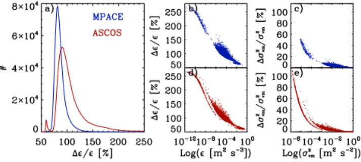
or radiosondes are expected to have a relatively small error, the primary contribution here is likely from variability of the wind speeds during the wind profiler’s averaging time pe-riod (∼30 min) or from temporal interpolation of radiosonde winds. Here we assume that this error is approximately 50 %. Time-height fields for both the fractional measurement er-ror in velocity variance and the fractional erer-ror in dissipation rate are shown for the 28 August 2008 case in Fig. 1b and d, respectively. This case suggests increased errors under con-ditions of low dissipation rate. More general results, derived from multiple days’ worth of retrievals for each experiment, are exhibited in Fig. 3. These demonstrate a clear increase in error as dissipation rate decreases. Additionally, distribu-tions of fractional error in dissipation rate show relatively more high errors during ASCOS relative to MPACE, in part due to a higher fractional occurrence of the lowest dissipa-tion rates. In general, fracdissipa-tional errors are less than 250 %, although these errors could be somewhat different if the con-tribution due to uncertainty in wind speed varies from the assumed 50 %. It is also important to note that the extent of fractional errors in dissipation rate is limited here because the radar measurements are limited to relatively large signals (i.e. SNR greater than−13 dB).
2.3 Evaluation measurements and methods
Before introducing specific data sets, it is important to note that because the dissipation rate values considered here oc-cur over as many as five orders of magnitude, the logarithms (base 10) of the dissipation rates are used in most figures, tables, and discussions. This logarithmic perspective more clearly reflects the differences and/or uncertainties in the data relative to their magnitude over a very wide range. To illus-trate this point, a factor of 2 difference at a dissipation rate of 1×10⁻⁶m2s−3 is much smaller than a factor of 2 dif-ference at a dissipation rate of 1×10⁻³m2s−3, while in a relative sense they are equivalent. This perspective should be kept in mind when interpreting the information provided in the following discussions. For example, a root mean squared (RMS) difference of 1.0 between two logarithmic data sets implies differences of an order of magnitude in the raw data, while an RMS of 0.6 implies differences of a factor of 4 (i.e. 100.6= 4.0).
During ASCOS, a tethered SkyDoc aerostat balloon was flown from a station on the sea-ice approximately 160 m from the icebreaker. Hanging 10 m below the balloon was an in-strument package that included a Gill Inin-struments Windmas-ter sonic anemomeWindmas-ter housed in an aerodynamic enclosure along with purpose-built control and data acquisition elec-tronics (hereafter referred to as the “tethersonde”). A serial communications interface allows the system to be configured from a laptop in the field, while data is recorded internally on a micro-SD data card. Power is provided from an exter-nal, rechargeable 12-V battery pack, allowing rapid replace-ment between flights and almost continuous operation. The
Fig. 3.Distributions of the theoretical fractional error in dissipation rate calculated using Eq. (7)(a), relationships between dissipation rate and the fractional error in dissipation rate (bandd), and rela-tionships between the velocity variance and the fractional error in velocity variance (cande) for all valid dissipation rate retrievals on the comparison days use in this study. In all cases, red represents ASCOS results while blue represents MPACE results.
sonic anemometer measures the 3 components of the turbu-lent wind at 40 Hz then internally averages these to 10 Hz before recording.
On a moving platform, measured wind components are contaminated by the motion and changing orientation of the sensor. Dissipation rate can be determined from the mea-sured power spectral density S without motion correcting the wind measurements by utilizing a portion of the iner-tial subrange at frequencies higher than those that charac-terize the platform motion (e.g. Yelland et al., 1994). Here, the portion of the spectrum used in these calculations is re-stricted to frequencies greater than 2 Hz. For a large fraction of its flight time, the tethersonde was operated in a profil-ing mode – ascendprofil-ing or descendprofil-ing at a mean rate of ap-proximately 0.3 m s−1. The averaging period used to calcu-late the dissipation rate is thus a tradeoff between minimizing the uncertainty in each individual estimate (longer averaging times) and localizing the estimate vertically (shorter averag-ing times). A 2-min averagaverag-ing period has been adopted here, providing a vertical resolution of approximately 36 m dur-ing profildur-ing, broadly comparable to the 45-m vertical reso-lution of the radar. Comparisons are made during cases on 24–30 August 2008.
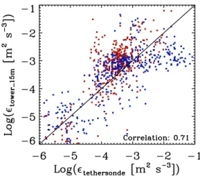
Fig. 4.Point-to-point comparisons of dissipation rate derived from the tethersonde and meteorological tower measurements at ASCOS. The tower measurements are made at 15 (blue) and 30 m (red). The one-to-one line is included.
is 0.75 log (m2s−3), which indicates that the RMS is on the order of a factor of 5.5 times the dissipation rate at any given value.
The error in individual dissipation rates derived from sonic anemometers is expected to be very small because the mea-surement error in S is much smaller than S itself. Thus, spread in the comparison is likely due to both the horizontal separation of the sensors and vertical averaging of the tether-sonde data in a near-surface environment that can have large vertical gradients in dissipation rate. To examine the spatial issues in more detail, a lag analysis was applied to the teth-ersonde and tower-mounted observations in this comparison as an approximation of spatial differences. The lag analysis effectively compares the dissipation rates determined from one 2-min sample with those from following samples made by the same sensor. Results are consistent for both tower and tethersonde measurements, showing RMS values of 0.3 and 0.36 log (m2s−3) at 2- and 4-min lag, respectively. These values indicate that a significant portion of the difference between tethersonde- and tower-derived dissipation rates is likely related to spatial differences.
For point-to-point comparisons and statistics relating the ASCOS radar retrievals and tethersonde measurements, the radar retrievals are simply averaged over the same 2-min time periods as the tethersonde measurements since the latter were typically made within a few hundred meters of the vertical radar beam. This approach has previously been used with the same tethersonde to evaluate dissipation rates from a ground-based Doppler lidar (O’Connor et al., 2010).
During MPACE, turbulent dissipation rate was derived from high frequency true air speed measurements made us-ing pitot tubes at both nose and wus-ing locations onboard the University of North Dakota Citation research aircraft. Turbu-lence calculations assume isotropy and are based on structure
Table 2.Statistics comparing dissipation rates derived from tether-sonde measurements with 15- and 30-m tower measurements during ASCOS. Statistics are representative of tower values within spec-ified ranges of the tethersonde-derived dissipation rates given in the left-most column. All statistics are computed using the loga-rithms (base 10) of the dissipation rates and include the total num-ber of observations (N), median (Med), interquartile range (IQR), mean absolute difference (MAD), root mean square difference (RMS), and relative bias between data sets (Bias). For these cal-culations: MAD =P
|x−y|/N, RMS = (P
[(x−y)2]/N)1/2, and Bias = 2.0/N·P
[(x−y)/(x+y)], wherexis the tethersonde data,
yis the tower data, andNis the number of samples. All values are in units of log (m2s−3)except forN and Bias. The latter can be thought of as a factor relative to the mean value in the range of in-terest. A positive bias in this case, due to the fact that the logarithms are themselves negative, indicates that the tower-derived dissipation rate is larger than that from the tethersonde.
Log(ε)Bin N Med IQR MAD RMS Bias −5.7 to−5.2 34 −5.3 0.63 0.43 0.54 0.04 −5.2 to−4.7 48 −5.3 0.96 0.51 0.62 −0.05 −4.7 to−4.2 36 −4.0 1.81 0.88 1.07 0.12 −4.2 to−3.7 133 −3.4 0.84 0.66 0.81 0.13 −3.7 to−3.2 260 −3.1 0.47 0.47 0.59 0.12 −3.2 to−1.2 261 −2.9 0.67 0.64 0.81 −0.07
All data 787 −3.1 0.91 0.59 0.75 0.04
functions applied to the airspeed measurements over running 10-s (∼800 m) windows reported every 1 s (e.g. Poellot and Grainer, 1991; Shupe et al., 2008b). Sources of noise or bias in the turbulence are due to noise in the airspeed measure-ments, which is low (M. Poellot, personal communication, 2007). Comparisons of dissipation rates derived from iden-tical measurements at the aircraft nose and wing show high consistency with a RMS difference of 0.23 log (m2s−3), or
less than a factor of 2 at any given dissipation rate, and a cor-relation coefficient of 0.92. This difference in measurements between the two aircraft locations provides an estimate of the measurement uncertainty in aircraft dissipation rates used here.
Fig. 5.Vertical profile comparisons of dissipation rate on specific days. In situ observations are given as individual points while radar retrievals are the mean (vertical line) and range (5th to 95th per-centiles as horizontal lines) of values derived over the time pe-riod of the in situ observations. Specific cases include:(a)19:00– 20:00 UTC on 5 October 2004 at MPACE; (b) 19:00–20:00 on 6 October at MPACE;(c)17:00 on 27 August to 05:00 on 28 Au-gust 2008 at ASCOS; and(d)00:00–12:00 on 29 August 2008 at ASCOS. For panels(a)and(b), the horizontal distance from the aircraft measurement to the vertical radar beam is designated by the color of each symbol.
3 Results
During the 28 August 2008 case at ASCOS the tethered bal-loon was flown through a series of three ascent-descent pat-terns up to heights of 500–600 m. Dissipation rates measured by the tethersonde system are shown in Fig. 1f, while radar-based retrievals subsampled at the same heights and 2-min time windows as the tethersonde measurements are given in Fig. 1e. The two independent measures of dissipation rate show broad agreement both in magnitude and in vertical and temporal changes observed during this case. Additionally, the full time-height display of radar retrievals (Fig. 1c) re-veals a wealth of additional detail that is not obtainable from the tethersonde measurements.
More detailed vertical profile comparisons in a range of conditions further reveal that the radar-based retrievals are able to capture the vertical turbulent structure with some in-tegrity. On 5 and 6 October 2004, the Citation aircraft flew multiple spiraling profiles near the NSA facility, for no more than one hour on each day, which offer a good opportunity for comparison with ground-based retrievals. Similarly, two cases were selected from the ASCOS experiment with mul-tiple tethered-balloon soundings. The time periods for these cases on 27–28 and 29 August 2008 were chosen such that the dissipation rate profiles were relatively consistent in time for up to 12 h according to the radar retrievals, with no major
Table 3.Statistics comparing radar retrievals of dissipation rate with in situ observations from aircraft at MPACE. All details are similar to Table 2 with the statistics computed for the radar retrievals within bin ranges defined by the aircraft values. A positive bias indicates that the radar retrieval is larger than the aircraft measurement.
Log(ε)Bin N Med IQR MAD RMS Bias −5.7 to−5.2 830 −5.1 0.48 0.45 0.59 0.08 −5.2 to−4.7 936 −4.8 0.55 0.40 0.51 0.05 −4.7 to−4.2 1095 −4.6 0.70 0.44 0.55 −0.01 −4.2 to−3.7 729 −4.2 0.91 0.49 0.62 −0.06 −3.7 to−3.2 762 −3.7 0.70 0.44 0.60 −0.10
All data 4921 −4.6 1.15 0.48 0.61 0.01
transitions such as the one shown in Fig. 1. For all of these cases, radar-derived dissipation rates sampled at all heights over the time periods when in situ observations were made are statistically represented in each panel of Fig. 5.
It is noteworthy that nearly all tethersonde and aircraft samples during these cases lie within the range (5th to 95th percentile) of retrieved dissipation rates. On 5 October 2004 and 27–28 August 2008 the retrievals indicate relatively little vertical change in turbulence distributions at altitudes below about 900 m, consistent with the in situ observations. On the other hand, during 6 October 2004 the retrievals successfully represent the observed turbulence minimum in the middle of the cloud layer, while on 5 October 2004 the retrievals cap-ture an observed increase and then decrease with ascending height near the cloud top. Lastly, while there were a few indi-vidual tethersonde measurements in disagreement, the radar suggests a diminishing amount of turbulence from 400 m down to the lower limit of the radar data at 100 m that is consistent with most of the observations on 29 August 2008. Point-to-point comparisons between radar retrieved and in situ observed dissipation rates demonstrate reasonable cor-respondence in a mean sense with the primary clusters of points falling along the one-to-one lines (Fig. 6). These com-parisons will be explored in more depth with the aid of scatter plots (Fig. 6), histograms (Fig. 7), and statistical summaries (Tables 3 and 4). The scatter plots and tables contain statisti-cal information characterizing subranges of the observed dis-sipation rates, while the histograms and tables contain statis-tical information characterizing the full comparison data sets. RMS differences, mean absolute differences (MAD), and rel-ative biases are computed according to the equations given in the caption for Table 2 using the logarithm (base 10) of the dissipation rates.
Fig. 6.Point-to-point comparisons of dissipation rate for all cases at (aandc) MPACE and (b andd) ASCOS. Statistics of the re-trieved data in bins of the in situ data are given as box-and-whisker plots that show the median (middle bar), 25th and 75th percentiles (ends of box), 5th and 95th percentiles (whiskers), and the mean as a symbol. Points in panel a are colored according to the horizon-tal distance between the aircraft observation and the vertical radar beam, points in panel b are colored according to the day of ob-servation during ASCOS, and points in panels c and d are colored according to the fractional error in dissipation rate calculated using Eq. (7). One-to-one lines are included in each panel.
highest and lowest observed dissipation rates. This bi-modal shape may be due to the presence of both weak, persistent background turbulence and more periodic but strongly forced turbulence regimes (e.g. Tjernstr¨om et al., 2009). RMS and MAD calculations indicate relative consistency across the range of values, with a typical RMS around 0.6 log (m2s−3), indicating general agreement in the raw data to within about a factor of 4. When considering the full dataset, the relative bias is very small and the correlation coefficient is 0.67. Rel-ative to the comparison between the two probes mounted on the same aircraft, the radar-aircraft comparison shows RMS values that are more than a factor of two larger. Individual point differences are often larger than the computed frac-tional error in the dissipation rate retrieval (Fig. 6c), suggest-ing that some component of the additional variability is due to variations in spatial sampling that are not a significant is-sue for the two aircraft probes.
The ASCOS data sets reveal a somewhat different story. First, the tethersonde observations follow a bi-modal dis-tribution (Fig. 7b). Remarkably, the dissipation rates of the two modes correspond quite well with the two primary modes observed by the aircraft during MPACE. However, the
Table 4.Statistics comparing radar retrievals of dissipation rate with in situ observations from the tethersonde at ASCOS. All details are similar to Table 2 with statistics computed for the radar retrievals within bin ranges defined by the tethersonde values. A positive bias indicates that the radar retrieval is larger than the tethersonde mea-surement.
Log(ε)Bin N Med IQR MAD RMS Bias −5.7 to−5.2 37 −5.5 1.77 0.89 1.04 0.01 −5.2 to−4.7 125 −5.0 1.42 0.80 1.11 −0.05 −4.7 to−4.2 205 −4.7 1.08 0.70 0.96 −0.05 −4.2 to−3.7 323 −3.8 0.94 0.56 0.75 0.02 −3.7 to−3.2 556 −3.4 0.74 0.43 0.54 0.01
All data 1368 −3.8 1.18 0.55 0.75 −0.01
Fig. 7.Distributions of dissipation rate for all cases at(a)MPACE and(b)ASCOS. In each panel, box-and-whisker plots show the me-dian (middle bar), 25th and 75th percentiles (ends of box), 5th and 95th percentiles (whiskers), and mean as a symbol.
occurrence frequencies for the two modes are substantially different; the MPACE aircraft observations do not show as many large values and have more of a tail towards smaller values relative to the ASCOS tethersonde measurements. Both in situ observations and radar retrievals indicate that the mean and maximum dissipation rates are larger for these subsets of observations at ASCOS relative to MPACE.
effective measurement limit leading to an overestimation. If this case is removed from consideration, the radar retrievals have little bias at low dissipation rates. In higher-turbulence conditions, the retrievals well represent the mean observed dissipation rates, with a very small positive bias, but still have a significant spread (Table 4). The RMS generally de-creases with increasing dissipation rate from values around 1.0 log (m2s−3)at the smallest rates to 0.5 log (m2s−3)at the largest. This trend is diminished somewhat, although still present, if the 30 August 2008 case is removed from con-sideration. Relative to the MPACE comparison, the ASCOS RMS values are larger in all ranges of dissipation rate except for the highest. For the whole ASCOS data set, the RMS is 0.75 log (m2s−3), which indicates differences of about a factor of 5.5 for the raw data. These differences are similar to, and even slightly smaller than, the observed differences between the tethersonde and tower measurements using the same type of sonic anemometer sensor. Only at low dissi-pation rates is the RMS between the radar and tethersonde data sets significantly larger than the RMS between the teth-ersonde and tower data sets, although, as noted above, some portion of this spread is due to apparent overestimates by the tethersonde at low dissipation rates.
4 Conclusions
Retrievals of turbulent dissipation rate from the time-variance of velocities measured by Doppler cloud radars in Arctic mixed-phase stratocumulus clouds have been evalu-ated against in situ measurements. This evaluation takes ad-vantage of two experiments. In the first, an instrumented teth-ered balloon was flown above a radar operated from the deck of an icebreaker embedded within the Arctic sea-ice pack. For the second, a research aircraft flew a number of horizon-tal legs and spiral profiles near a ground-based radar operated in Barrow, Alaska, USA. These comparison data sets offer a unique opportunity to evaluate dissipation rate retrievals in Arctic clouds.
When comparing point-to-point measurements for both experiments, there is significant scatter as might be expected due to drastically different sample volumes that are some-times in significantly different locations. The absolute uncer-tainty in radar-based retrievals is difficult to determine be-cause the in situ observations themselves contain substantial, sometimes uncharacterized, uncertainties. In the case of the aircraft observations, comparisons between two similar sen-sors operated in tandem on the same platform indicate RMS differences of nearly a factor of two, which might be repre-sentative of the uncertainty associated with identical mea-surements made in near identical locations. However, this does not provide any information on the additional uncer-tainties that might be caused by spatial separation or sam-pling differences. Dissipation rates derived using nearly iden-tical sonic anemometer measurements on a tethersonde and
on 15- and 30-m towers at spatial distances of 225–275 m during ASCOS showed RMS differences of a factor of six. A time lag analysis conducted using the tower and tethersonde measurements suggests that as much as half of the RMS dif-ference between two different measurements could be due to spatial inhomogeneities in the turbulence field. Thus, while the relative magnitudes of observational uncertainties from different sources are not known absolutely, these compar-isons of in situ measurements provide some important con-text for the evaluation of radar-based retrievals.
Comparisons between the radar retrievals and in situ mea-surements offer insight into how well the retrievals are able to capture the basic structure and magnitude of turbulent dis-sipation rates relative to the more traditional measures of the quantity. In some cases, the comparisons paint incon-sistent pictures. For example, under low-turbulence condi-tions, radar retrievals appear to overestimate the dissipation rate relative to nearby aircraft measurements but possibly un-derestimate these rates relative to tethersonde measurements. For the full comparison data sets, the retrievals also show a much wider range of values than the tethersonde, but a nar-rower range than the aircraft, in spite of having very small net biases in both cases.
The comparison data sets have RMS differences (for log-arithmic data) of 0.61 and 0.75 log (m2s−3)for the aircraft and tethersonde comparisons, respectively. These values are consistent with variability among techniques on the order of a factor of 4–6 for non-logarithmic dissipation rates. For con-text, these differences are no larger than those observed be-tween the spatially separated, sonic-anemometer-based esti-mates of dissipation rate at ASCOS. Based on the lag anal-ysis results for those sonic-anemometer-based estimates, it is anticipated that as much as half of the variability between radar retrievals and verification data is due to spatial differ-ences in sampling. These results therefore suggest typical re-trieval uncertainties on the order of a factor of 2–3. Much, but not all, of this remaining variability can be explained directly by computed retrieval errors resulting from uncertainty in de-termining the velocity variance and horizontal wind speed (e.g. Fig. 3).
There are some further considerations that might explain additional small sources of bias and uncertainty. For cases of apparent retrieval underestimation, such as for the high-est dissipation rates observed at MPACE and the lowhigh-est rates observed at ASCOS, this underestimate could be related to the radar sample time being too long, such that the effective sampling length, Ll, extends beyond the scales associated
remained within the inertial subrange (e.g. Bouniol et al., 2003). Furthermore, some component of the bias in these cases may be due to the in situ measurements (e.g. the 30 Au-gust 2008 case at ASCOS).
On the other hand, erroneously large dissipation rates might be inferred if the variance of Doppler velocity mea-surements is larger than the variance due solely to turbulence. As noted by Lothon et al. (2005) and exhibited in Eq. (1), additional variance could be due to contributions from mi-crophysics and/or covariance between turbulent motions and microphysics. However, in their analyses of drizzling stra-tocumulus, Lothon et al. (2005) found that the microphysics-turbulence correlations actually lead to an underestimation of the dissipation rate. Power spectra computed from radar ve-locity time series (Fig. 2) follow the expected Kolmogorov form of the inertial subrange, suggesting that microphysi-cal variance typimicrophysi-cally did not contribute significantly to the variance in these comparisons. Lastly, additional scatter may have been introduced into these comparisons by significant differences in the effective sample volumes among the in-struments.
In spite of the differences that are observed, two primary results can be drawn from this evaluation. First, the differ-ences between radar-based estimates of dissipation rate ap-pear to be no larger than differences between rates derived from different sonic anemometer measurements at similar spatial separations. Second, it is clear that the radar-based retrievals contain important qualitative information on the vertical structure of turbulent dissipation rate within Arc-tic mixed-phase stratocumulus clouds. For example, the re-trievals are able to reveal the presence, or lack thereof, of vertical turbulence gradients. Additionally, a strength of the radar retrieval approach relative to the in situ approaches is that it provides continuous, coordinated profiling of both turbulence and cloud microphysical properties within the cloudy atmosphere. This information has implications for the ability to statistically characterize and understand processes within these clouds. Specifically, knowledge of turbulence profiles offers insight into the source of turbulent energy to the cloud layer, which interacts with cloud and thermody-namic properties and ultimately plays a key role in the cloud life cycle.
Acknowledgements. This research was supported by the Office of
Science (BER), US Department of Energy (grant DE-SC0007005), the US National Science Foundation (grant ARC1023366), and the UK Natural Environment Research Council (NERC, grants NE/E010008/1 and NE/H02168X/1). Barrow and MPACE data were obtained from the Atmospheric Radiation Measurement Program archive. Many thanks to the MPACE project and aircraft leaders, Hans Verlinde and Michael Poellot. ASCOS was supported by the Knut and Alice Wallenberg Foundation, the DAMOCLES Integrated Research Project from the European Union 6th Frame-work Program, the US National Science Foundation, and the UK Natural Environment Research Council. The ASCOS cloud
radar was provided by the US National Oceanic and Atmospheric Administration. The tethered balloon was provided by the NERC National Centre for Atmospheric Science. Special thanks go to the ASCOS team for collecting the turbulence datasets and overall project implementation, particularly Cathryn Birch, Paul Johnston, Caroline Leck, Thorsten Mauritsen, Sarah Norris, Ola Persson, Joseph Sedlar, and Michael Tjernstr¨om.
Edited by: M. Tjernstr¨om
References
Banakh, V. A. and Smalikho, I. N.: Estimation of turbulent energy dissipation rate from data of pulse Doppler lidar, Atmos. Ocean. Opt., 10, 957–965, 1997.
Bouniol, D., Illingworth, A. J., and Hogan, R. J.: Deriving turbu-lent kinetic energy dissipation rate within clouds using ground based 94 GHz radar, Preprints, 31st Conf. on Radar Meteorol-ogy, Seattle, WA, Am. Meteor. Soc., 193–196, available at: http: //ams.confex.com/ams/pdfpapers/63826.pdf, 2003.
Bretherton, C. S., Uttal, T., Fairall, C. W., Yuter, S. E., Weller, R. A., Baumgardner, D., Comstock, K., Wood, R., and Raga, G. B.: The EPIC 2001 Stratocumulus Study, B. Am. Meteorol. Soc., 85, 967–977, 2004.
Brewster, K. A. and Zrnic, D. S.: Comparison of eddy dissipation rates from spatial spectra of Doppler velocities and Doppler spec-trum widths, J. Atmos. Ocean.-Tech., 3, 440–452, 1986. Caughey, S. J., Wyngaard, J., and Kaimal, J.: Turbulence in the
evolving stable boundary layer, J. Atmos. Sci., 36, 1041–1052, 1979.
Chen, W. Y.: Energy dissipation rates of free atmospheric turbu-lence, J. Atmos. Sci., 31, 2222–2225, 1974.
Clothiaux, E. E., Ackerman, T. P., Mace, G. G., Moran, K. P., Marc-hand, R. T., Miller, M. A., and Martner, B. E.: Objective deter-mination of cloud heights and radar reflectivities using a combi-nation of active remote sensors at the ARM CART sites, J. Appl. Meteorol. Clim., 39, 645–665, 2000.
Cohn, S. A.: Radar measurements of turbulent eddy dissipation rate in the troposphere: A comparison of techniques, J. Atmos. Ocean.-Tech., 12, 85–95, 1995.
Comstock, J. M., D’Entremont, R., DeSlover, D., Mace, G. G., Ma-trosov, S. Y., McFarlane, S. A., Minnis, P., Mitchell, D., Sassen, K., Shupe, M. D., Turner, D. D., and Wang, Z.: An intercompari-son of microphysical retrieval algorithms for upper-tropospheric ice clouds, B. Am. Meteorol. Soc., 88, 191–204, 2007.
Deng, M. and Mace, G. G.: Cirrus microphysical properties and air motion statistics using cloud radar Doppler moments. Part I: Algorithm description, J. Appl. Meteorol. Clim., 45, 1690–1709, 2006.
Fairall, C. W., Markson, R., Schacher, G. E., and Davidson, K. L.: An aircraft study of turbulence dissipation rate and temperature structure function in the unstable marine atmospheric boundary layer, Bound.-Lay. Meteorol., 18, 453–469, 1980.
Frehlich, R.: Estimation of velocity error for Doppler lidar measure-ments, J. Atmos. Ocean. Tech., 18, 1628–1639, 2001.
Frisch, A. S. and Clifford, S. F.: A study of convection capped by a stable layer using Doppler radar and acoustic echo sounders, J. Atmos. Sci., 31, 1622–1628, 1974.
Frisch, A. S. and Strauch, R. G.: Doppler radar measurements of tur-bulent kinetic energy dissipation rates in a northeastern Colorado convective storm, J. Appl. Meteorol., 15, 1012–1017, 1976. Gossard, E. E., Snider, J. B., Clothiaux, E. E., Martner, B., Gibson,
J. S., Kropfli, R. A., and Frisch, A. S.: The potential of 8-mm radars for remotely sensing cloud drop size distributions, J. At-mos. Ocean.-Tech., 14, 76–87, 1997.
Illingworth, A. J., Hogan, R. J., O’Connor, E. J., Bouniol, D., Brooks, M. E., Delenoe, J., Donovon, D. P., Eastment, J. D., Gaussiat, N., Goddard, J. W. F., Haeffelin, M., Klein Baltink, H., Krasnov, O. A., Pelon, J., Piriou, J.-M., Protat, A., Russchen-berg, H. W. J., Seifert, A., Tompkins, A. M., van Zadelhoff, G.-J., Vinit, F., Willen, U., Wilson, D. R., and Wrench, C. L.: Cloud-net – Continuous evaluation of cloud profiles in seven operational models using ground-based observations, B. Am. Meteorol. Soc., 88, 883–898, 2007.
Kollias, P., Albrecht, B. A., Lhermitte, R., and Savtchenko, A.: Radar observations of updrafts, downdrafts, and turbulence in fair-weather cumuli, J. Atmos. Sci., 58, 1750–1766, 2001. Kollias, P., Miller, M. A., Luke, E. P., Johnson, K. L., Clothiaux,
E. E., Moran, K. P., Widener, K. B., and Albrecht, B. A.: The Atmospheric Radiation Measurement Program cloud profiling radars: Second-generation sampling strategies, processing, and cloud data products, J. Atmos. Ocean.-Tech., 24, 1199–1214, 2007.
Lenschow, D. H., Wulfmeyer, V., and Senff, C.: Measuring second-through fourth-order moments in noisy data, J. Atmos. Ocean.-Tech., 17, 1330–1347, 2000.
Lothon, M., Lenschow, D. H., Leon, D., and Vali, G., Turbulence measurements in marine stratocumulus with airborne Doppler radar, Q. J. Roy. Meter. Soc., 131, 2063–2080, 2005.
Luke, E., Kollias, P., and Shupe, M. D.: Detection of supercooled liquid in mixed-phase clouds using radar Doppler spectra, J. Geo-phys. Res., 115, D19201, doi:10.1029/2009JD012884, 2010. Moran, K. P., Martner, B. E., Post, M. J., Kropfli, R. A., Welsh,
D. C., and Widener, K. B.: An unattended cloud-profiling radar for use in climate research, B. Am. Meteorol. Soc., 79, 443–455, 1998.
Muschinski, A., Frehich, R., Jensen, M., Hugo, R., Hoff, A., Eaton, F., and Balsley, B.: Find-scale measurements of turbu-lence in the lower troposphere: An intercomparison between a kite- and balloon-borne, and a helicopter-borne measurement system, Bound.-Lay. Meteorol., 98, 219–250, 2001.
Nicholls, S. and Turton, J. D.: An observational study of the struc-ture of stratiform cloud sheets: Part 2. Entrainment, Q. J. Roy. Meteor. Soc., 112, 461–480, 1986.
O’Connor, E. J., Hogan, R. J., and Illingworth, A. J.: Retrieving stratocumulus drizzle parameters using Doppler radar and lidar, J. Appl. Meteorol., 44, 12–27, 2005.
O’Connor, E. J., Illingworth, A. J., Brooks, I. M., Westbrook, C. D., Hogan, R. J., Davis, F., and Brooks, B. J.: Balloon-borne in-situ evaluation of a fast method for estimating dissipation rate from a vertically-pointing Doppler lidar, J. Atmos. Ocean.-Tech., 27, 1652–1664, 2010.
Poellot, M. R. and Grainger, C. A.: A comparison of several air-borne measures of turbulence. Paper presented at 4th Interna-tional Conference on Aviation Weather Systems, American Me-teorological Society, Paris, France, 1991.
Rogers, R. R. and Tripp, B. R.: Some radar measurements of turbu-lence in snow, J. Appl. Meteorol., 3, 603–610, 1964.
Sedlar, J., Tjernstr¨om, M., Maurtisen, T., Shupe, M. D., Brooks, I. M., Persson, P. O. G., Birch, C. E., Leck, C., Sirevaag, A., and Nicolaus, M.: A transitioning Arctic surface energy budget: the impacts of solar zenith angle, surface albedo and cloud radiative forcing, Clim. Dynam., 37, 1643–1660, 2011.
Shupe, M. D.: A ground-based multiple remote-sensor cloud phase classifier, Geophys. Res. Lett., 34, L22809, doi:10.1029/2007GL031008, 2007.
Shupe, M. D., Kollias, P., Matrosov, S. Y., and Schneider, T. L.: De-riving mixed-phase cloud properties from Doppler radar spectra, J. Atmos. Ocean.-Tech., 21, 660–670, 2004.
Shupe, M. D., Matrosov, S. Y., and Uttal, T.: Arctic mixed-phase cloud properties derived from surface-based sensors at SHEBA, J. Atmos. Sci., 63, 697–711, 2006.
Shupe, M. D., Daniel, J. S., de Boer, G., Eloranta, E. W., Kollias, P., Luke, E., Long, C. N., Turner, D. D., and Verlinde, J.: A focus on mixed-phase clouds: The status of ground-based observational methods, B. Am. Meteorol. Soc., 89, 1549–1562, 2008a. Shupe, M. D., Kollias, P., Poellot, M., and Eloranta, E.: On deriving
vertical air motions from cloud radar Doppler spectra, J. Atmos. Ocean.-Tech., 25, 547–557, 2008b.
Shupe, M. D., Kollias, P., Persson, P. O. G., and McFarquhar, G. M.: Vertical motions in Arctic mixed-phase stratiform clouds, J. Atmos. Sci., 65, 1304–1322, 2008c.
Sreenivasan, K. R.: On the universality of the Kolmogorov constant, Phys. Fluids, 7, 2778–2784, 1995.
Stevens, B.: Entrainment in stratocumulus topped mixed layers, Q. J. Roy. Meteor. Soc., 128, 2663–2690, 2002.
Taylor, G. I.: Statistical theory of turbulence, P. Roy. Soc. A-Math. Phy., 151, 421–444, 1935.
Tjernstr¨om, M., Balsley, B. B., Svensson, G., and Nappo, C. J.: The effects of critical layers on residual layer turbulence, J. Atmos. Sci., 66, 468–480, 2009.
Verlinde, J., Harrington, J. Y., McFarquhar, G. M., Yannuzzi, V. T., Avramov, A., Greenberg, S., Johnson, N., Zhang, G., Poellot, M. R., Mather, J. H., Turner, D. D., Eloranta, E. W., Zak, B. D., Prenni, A. J., Daniel, J. S., Kok, G. L., Tobin, D. C., Holz, R., Sassen, K., Spangenberg, D., Minnis, P., Tooman, T. P., Ivey, M. D., Richardson, S. J., Bahrmann, C. P., Shupe, M., Demott, P. J., Heymsfield, A. J., and Schofield, R.: The Mixed-Phase Arctic Cloud Experiment (M-PACE), B. Am. Meteorol. Soc., 88, 205– 220, 2007.