www.atmos-chem-phys.net/14/7869/2014/ doi:10.5194/acp-14-7869-2014
© Author(s) 2014. CC Attribution 3.0 License.
Reconciling aerosol light extinction measurements from spaceborne
lidar observations and in situ measurements in the Arctic
M. Tesche1, P. Zieger1, N. Rastak1, R. J. Charlson2, P. Glantz1, P. Tunved1, and H.-C. Hansson1
1Department of Applied Environmental Science, Stockholm University, Stockholm, Sweden 2Department of Atmospheric Sciences, University of Washington, Seattle, WA 98195, USA
Correspondence to:M. Tesche (matthias.tesche@itm.su.se)
Received: 10 February 2014 – Published in Atmos. Chem. Phys. Discuss.: 4 March 2014 Revised: 11 June 2014 – Accepted: 1 July 2014 – Published: 8 August 2014
Abstract. In this study we investigate to what degree it is possible to reconcile continuously recorded particle light ex-tinction coefficients derived from dry in situ measurements at Zeppelin station (78.92◦N, 11.85◦E; 475 m above sea level), Ny-Ålesund, Svalbard, that are recalculated to ambient rel-ative humidity, as well as simultaneous ambient observa-tions with the Cloud-Aerosol Lidar with Orthogonal Polar-ization (CALIOP) aboard the Cloud-Aerosol Lidar and In-frared Pathfinder Satellite Observations (CALIPSO) satellite. To our knowledge, this represents the first study that com-pares spaceborne lidar measurements to optical aerosol prop-erties from short-term in situ observations (averaged over 5 h) on a case-by-case basis. Finding suitable comparison cases requires an elaborate screening and matching of the CALIOP data with respect to the location of Zeppelin sta-tion as well as the selecsta-tion of temporal and spatial averag-ing intervals for both the ground-based and spaceborne ob-servations. Reliable reconciliation of these data cannot be achieved with the closest-approach method, which is often used in matching CALIOP observations to those taken at ground sites. This is due to the transport pathways of the air parcels that were sampled. The use of trajectories allowed us to establish a connection between spaceborne and ground-based observations for 57 individual overpasses out of a total of 2018 that occurred in our region of interest around Sval-bard (0 to 25◦E, 75 to 82◦N) in the considered year of 2008. Matches could only be established during winter and spring, since the low aerosol load during summer in connection with the strong solar background and the high occurrence rate of clouds strongly influences the performance and reliability of CALIOP observations. Extinction coefficients in the range of 2 to 130 Mm−1at 532 nm were found for successful matches
with a difference of a factor of 1.47 (median value for a range from 0.26 to 11.2) between the findings of in situ and space-borne observations (the latter being generally larger than the former). The remaining difference is likely to be due to the natural variability in aerosol concentration and ambient rela-tive humidity, an insufficient representation of aerosol parti-cle growth, or a misclassification of aerosol type (i.e., choice of lidar ratio) in the CALIPSO retrieval.
1 Introduction and motivation
Understanding and quantifying the climatic effects of natural and anthropogenic aerosols from direct observations requires a combination of data from a variety of instruments that usu-ally apply very different measurement techniques. For ex-ample, ground-based in situ measurements of aerosol opti-cal, microphysiopti-cal, and chemical properties (that are usually carried out with very high temporal resolution but only at a limited number of locations) can be combined with satellite observations or aircraft measurements (that generally pro-vide us with better spatial data coverage but are limited in temporal resolution and/or detail). The combination of such data needs to overcome differences in measurement time, lo-cation, and measured quantity. This poses the fundamental problem of relating point-sampling data to either spatially resolved data with poor temporal coverage or airborne mea-surements without profile information. Four issues arise:
1. Differences in measurement techniques:different
be of optical properties as well as physical and chemi-cal properties that can be transformed via theory or em-pirical data (i.e., parameterization) to optical properties (and vice versa).
2. Spatial resolution:location and spatial resolution of the
aerosol measurements are different. In situ observations are often point measurements, while the swath width of passive satellite sensors can extend over up to a few thousand kilometers. In addition, active satellite sensors with narrow footprints often do not cover exactly the lo-cation where the in situ observations are performed. It can also happen that clouds obstruct the wide field of view of a spaceborne sensor. If the satellite data were taken at a distance away from the ground site, it is also necessary to consider the time difference as a lead or a lag of timing.
3. Hygroscopicity:the thermodynamic state of the air
(es-pecially the relative humidity, RH) has a strong effect on the aerosol optical properties (particularly in the lower marine troposphere) and is different for the dif-ferent observations. Remote sensing of aerosols is nor-mally performed under ambient conditions (i.e., within the atmosphere), while most in situ instruments sample the aerosol under dry conditions with RH<30–40 %
(WMO, 2003).
4. Temporal resolution: the time periods over which the
observations are averaged may be various. Short tempo-ral averages (i.e., a few hours) complicate a comparison since such an effort is only meaningful when the differ-ent sensors actually observe the same air mass. Long-term averages (i.e., monthly means), on the other hand, can generate arbitrary coherence of the data – especially when the considered data sets are of different size. It is necessary to utilize these simultaneous but disparate data to be able to perform a closure study for the validation of remote-sensing data with independent in situ measure-ments and vice versa. Such closure studies are important not only for validating the retrievals of aerosol optical thickness (AOT) or the aerosol extinction coefficient but also for inves-tigating how the measured quantities are apportioned to dif-ferent types of aerosol, e.g., how large the anthropogenic in-fluence is on the optical properties of the atmosphere and thus the radiation balance. For this we have to be able to demon-strate that the measurement systems actually are sensing the same entity. The practical reality (i.e., it is not a simple mat-ter to combine the in situ and satellite data) is made into a doable but challenging task by recognition at the outset that both the spaceborne and the in situ instrument are well-tested devices that are operating correctly within the scope of their capabilities. Thus, the effort described here is not the usual
ground truthsort of activity done in order to constrain
mea-surement uncertainties. Rather, we intend to devise methods to bring the data sets into concordance.
Here, we consider in situ measurements performed at the Arctic station at Mt. Zeppelin (78.92◦N, 11.85◦E; 474 m above sea level), Svalbard, in comparison with data taken simultaneously (or nearly so) with the Cloud-Aerosol Lidar with Orthogonal Polarization (CALIOP) aboard the Cloud-Aerosol Lidar and Infrared Pathfinder Satellite Observations (CALIPSO; Winker et al., 2009) satellite. CALIPSO is oper-ating in near-polar orbit at an altitude of about 705 km.
In situ instruments usually measure aerosol properties un-der dry conditions with a RH of 10–30 % in an indoor labora-tory, while ambient conditions are usually associated with a much higher RH of up to 100 %. Hence, in situ measurements need to be transformed to ambient conditions by means of di-rect RH-dependent measurements or a microphysical particle model to account for the loss in particle size due to drying the aerosol particles (Tang and Munkelwitz, 1994; Tang, 1996; Zieger et al., 2013). On the other hand, ambient aerosol ex-tinction coefficients can be measured directly, for instance with active optical remote-sensing techniques such as lidar or differential optical absorption spectroscopy (DOAS). Pre-vious closure studies have shown that reasonable agreement is found between results obtained from remote sensing of aerosols and findings from in situ observations when the ef-fect of relative humidity has been accounted for (Hoff et al., 1996; Masonis et al., 2002; Zieger et al., 2011, 2012; Hoff-mann et al., 2012; Ziemba et al., 2013; Skupin, 2014). How-ever, studies in the literature mainly deal with a few single cases during intensive field campaigns rather than systematic comparisons of multiyear data sets.
The clean environment of the Arctic is very sensitive to anthropogenic impacts. Arctic aerosol conditions are also strongly influenced by regional meteorology (Eneroth et al., 2003; Stock, 2014), which controls the RH of the air. Changes in this parameter have a huge influence on aerosol particle size and thus light scattering (Zieger et al., 2010, 2013) and cloud formation (Mauritsen et al., 2011) in this region. Optical properties and concentrations of Arctic aerosols have been measured at Ny-Ålesund, Svalbard, with in situ instruments (Covert and Heintzenberg, 1993; Ström et al., 2003; Tunved et al., 2013) and by means of remote sens-ing (Herber et al., 2002; Hoffmann et al., 2009, 2012; Tomasi et al., 2007, 2012) for several years.
4 April 2009 could be reconciled to a factor of ca. 2 with smaller lidar-derived values compared to the in situ measure-ments.
The use of the spaceborne CALIPSO lidar has the poten-tial to overcome the altitude limitations since its observa-tions extend all the way down to the Earth’s surface. The high frequency of overpasses at high latitudes makes it at-tractive to consider the possibility of a combined analysis of ground-based in situ and spaceborne lidar measurements in the Arctic. In principle, such an analysis connects informa-tion on the vertical and horizontal aerosol distribuinforma-tion from the CALIPSO satellite data to the more specific information about aerosol microphysical and chemical properties at the surface. In situ measurements are limited to a few measure-ment locations, while satellites can (in principle) view the exact same volume of air that is being sampled at the sur-face. Satellite sensors also have vastly larger fields of view and allow for global or near-global data coverage. Conse-quently, they have a strong potential to extend the findings of in situ measurements in space besides giving information on aerosol optical properties. In the same way, findings from detailed in situ measurements can add further depth to the satellite observations.
Di Pierro et al. (2013) used these advantages to perform a comprehensive study of the spatial and seasonal distribu-tion of Arctic aerosols based on optical properties observed by CALIOP between 2006 and 2012. The authors introduce an empirical correction that accounts for the different mea-surement sensitivity during day and night – a crucial factor when it comes to summertime CALIOP observations in the Arctic. The authors found CALIOP aerosol extinction in the Arctic to be on the same order of magnitude as nephelometer observations at Barrow and Alert, with the latter being trans-formed to ambient RH. However, in addition to using highly averaged data (i.e., monthly and seasonal mean values) the averaging methodology of Di Pierro et al. (2013) applies a detection frequency that is defined as the ratio of the num-ber of height bins with detected aerosol layers to the total number of height bins in a given area and time period. This procedure is likely to decrease the magnitude of the obtained mean extinction profiles by introducing zero-values into the averaging. In fact, the authors show that the mean CALIOP extinction profile obtained for a comparison to measurements with a high-spectral-resolution lidar (HSRL) at Eureka yields much smaller values than the ground-based HSRL observa-tions. Di Pierro et al. (2013) also provide the reader with the seasonal variation of CALIOP-derived mean extinction co-efficients for different atmospheric layers. Their values for the layer from the surface to 2 km height are a maximum at around 10 Mm−1 in March for the Atlantic sector which is
most representative of the conditions at Svalbard. This re-lates to a maximum AOT of 0.02 for the polluted spring sea-son if we assume that the majority of aerosols are present within this 2 km deep layer. Such a value is similar to what is observed in the Arctic troposphere around Svalbard during
the clean summer season (Glantz et al., 2014). Note that it is more likely that the aerosol-containing planetary bound-ary layer at Svalbard is between 0.5 and 1.0 km deep – which would decrease the maximum AOT as derived from the val-ues presented in Di Pierro et al. (2013) even further. This discrepancy calls for a more detailed investigation of the fac-tors that influence the reconciliation of extinction coefficients from ground-based and spaceborne observations. We will re-turn to this point in the conclusion.
A description of the instrumentation and the data process-ing used in this study is presented in Sect. 2. Section 3 de-scribes the methodology for relating segments of individual CALIPSO overpasses to in situ measurements at Zeppelin station. The findings of the comparison for the year 2008 are discussed in Sect. 4. The paper ends with a summary and conclusions in Sect. 5.
2 Instrumentation and methods
2.1 In situ measurements at Zeppelin station
The aerosol in situ instruments at Zeppelin station include a differential mobility particle sizer (DMPS), for measuring the particle size distribution in the mobility diameter range from 10 to 790 nm (time resolution of 20 min); a particle soot absorption photometer (PSAP) for measurements of par-ticle light absorption coefficients at 525 nm (time resolution of 60 min) on a filter; and an integrating nephelometer (TSI model 3563) for measurements of particle light-scattering coefficients at the wavelengths of 450, 550, and 700 nm (time resolution of 10 min) (Ström et al., 2003; Tunved et al., 2013). The nephelometer measurements were corrected for the truncation error and lamp non-idealities according to An-derson et al. (1998). All in situ instruments are placed indoors and connected to an inlet without a particle size cut.
The location of Zeppelin station at 79◦N imposes a se-vere climatic situation, with usually low outside temperature (from−25 to +15◦C) and correspondingly high RH, often
near or at 100 %. The in situ instruments in the laboratory are operated at an ordinary room temperature of about 20◦C. Hence, sampled air is heated by as much as 40 K during its transit into the laboratory. Continuous aerosol in situ ob-servations are usually performed under dry conditions with RH<30–40 % in order to avoid the influence of water
up-take on the aerosol optical properties and to keep the mea-surements at different ambient RH and at different sites com-parable (WMO, 2003). The humidity effect on the scattering properties of the aerosol has to be accounted for if results are to represent actual atmospheric conditions.
Measurements with a humidified nephelometer operating at RH between 20 and 95 % were carried out between 15 July 2008 and 12 October 2008 at Zeppelin station (Zieger et al., 2010). A comparison to Zeppelin’s dry nephelometer (op-erating at RH<20%) showed that the ambient scattering
coefficients at RH=85% were on average about 3 times
higher than the scattering coefficients of the dried aerosol sample (Zieger et al., 2013). Direct measurements of the scat-tering enhancement factor were only available for 91 days in 2008.
2.2 Transferring measured dry parameters to ambient conditions
Hourly measurements of outdoor humidity at Zeppelin sta-tion are available to transform the dry in situ measure-ments to ambient conditions. This is done following two ap-proaches by using (1) the chemical composition of the par-ticles in combination with the particle size distribution from the DMPS as input to a hygroscopicity model and (2) the di-rect measurements of scattering and absorption coefficients from the nephelometer and PSAP in combination with a scat-tering enhancement factor f(RH). Cases with ambient RH
larger than 95 % were considered to be measurements within clouds or fog and were thus excluded from the procedure.
2.2.1 Site-specific hygroscopicity model
Dry size distributions are transformed to ambient conditions and then used as input for a Mie-scattering model to obtain ambient aerosol optical properties. For a detailed description of this procedure we refer the reader to Rastak et al. (2014), but a brief summary is given here.
Hygroscopicity effects are accounted for with the help of
κ-Köhler theory (Kreidenweis et al., 2005; Petters and
Krei-denweis, 2007). The aerosol growth factor is derived by com-bining the individual aerosol volume fractions obtained from the analysis of chemical samples collected at Ny-Ålesund with the hygroscopicity parameterκ of the respective
com-ponents available in the literature. The comcom-ponents consid-ered in this study are water-soluble and insoluble organics, ammonium sulfate, sea salt, and black carbon.
Ambient aerosol scattering, absorption, and extinction co-efficients are obtained from the humidified aerosol size dis-tribution and refractive index by means of Mie-scattering theory. All optical properties are calculated at a wavelength of 550 nm and with a temporal resolution of 1 h. Note that absorption contributes less than 5 % to the ambient extinc-tion coefficient of Arctic aerosols (Eleftheriadis et al., 2009; Zieger et al., 2010). This is in agreement with the PSAP measurements at Zeppelin. The effect of light absorption decreases even further when ambient extinction coefficients are considered. The uncertainties of a misrepresentation of aerosol light absorption become negligible when put into the
context of the challenges imposed by the comparison proce-dure described in Sect. 3.
A validation of the microphysical model is presented in Rastak et al. (2014). Dry aerosol scattering coefficients mea-sured by the nephelometer agree with those calculated from the particle size distributions (slope close to unity, R2=
0.95). A comparison between humidified scattering
coeffi-cients and measurements with the humidified nephelometer during the 91 days of parallel operation (Zieger et al., 2010) showed a slight tendency of the model to underestimate the measurements withR2=0.64 (Rastak et al., 2014). The
en-hancement factorf(RH) is the ratio of ambient to dry
ex-tinction coefficients. Values of f (RH)=4.30±2.26 with
a range from 1.5 to 12.5 were found when relating the re-sults obtained from the humidified size distribution to the dry nephelometer measurements for the year 2008. This is in agreement with the findings of Zieger et al. (2010) for Arctic aerosols at ambient RH at Zeppelin station.
The humidification of the particle number size distribution obtained with the DMPS leads to an increase of the parti-cle effective (surface-weighted) radius from 0.14±0.02 to
0.23±0.04 µm (yearly average, not shown). This moves the
aerosol from an optically ineffective state to a size range in which they are more efficient in interacting with visible light. Contributions of particles larger than the maximum DMPS size bin would lead to an overall increase in the effective ra-dius and thus would further improve the light-scattering effi-ciency of the probed aerosol.
2.2.2 Dry aerosol optical measurements and range of observedf(RH)
The DMPS measurements used in the previous section only cover particles up to a diameter of 790 nm and provide no information on the concentration of larger particles. Particles in the coarse mode can have a large effect on the overall ex-tinction coefficient due to their size and increased exex-tinction efficiency, although their concentration might be very low. Hence, missing even low concentrations of coarse particles can cause an underestimation of the aerosol scattering and extinction coefficients by as much as 30 %. In addition, it is more straightforward to determine ambient extinction coef-ficients directly from the nephelometer measurements if the scattering enhancement factor is known or can be estimated within a reasonable range of values.
Therefore, ambient extinction coefficients were also cal-culated using the dry absorption and scattering coefficients measured with the PSAP and nephelometer, respectively, together with scattering enhancement factors that represent the median, minimum, and maximum effect of hygroscopic growth on light scattering. Values of γ=0.57, 0.35, and
0.85, respectively, were used to obtain the scattering en-hancement factor for ambient RH asf (RH)=(1−RH)−γ
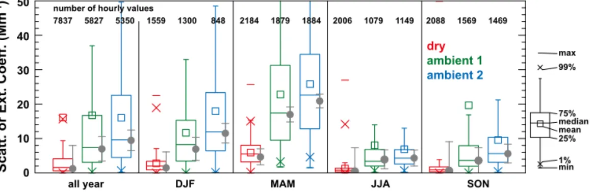
all year
0 10 20 30 40 50
Scatt. or Ext. Coeff. (Mm
-1)
DJF MAM JJA SON
dry ambient 1 ambient 2
max
min mean median
1% 99%
75%
25% number of hourly values
1569 1469 2088
1079 1149 2006
1879 1884 2184
1300 848 1559
5827 5350 7837
Figure 1. Statistical overview of the dry scattering (red) and ambient extinction coefficients at 550 nm based on hourly measurements
at Zeppelin station in 2008 according to the entire year and the different seasons: winter (DJF), spring (MAM), summer (JJA), and fall (SON). The ambient extinction coefficients refer to the results obtained by using humidified size distributions from DMPS measurements in combination with Mie-scattering theory (ambient 1, green) and the dry nephelometer and PSAP measurements in combination with a scattering enhancement factor derived for a meanγ of 0.57 (ambient 2, blue). The numbers at the top of the figure mark the number of
available hourly measurements. The difference in data availability for dry scattering and ambient extinction coefficients is the consequence of cloud screening and an absence of input data required for humidity correction.
2.2.3 Dry vs. ambient optical properties
The box plots in Fig. 1 show the importance of transform-ing dry optical properties to ambient conditions. About 75 % of the hourly aerosol scattering coefficients at 550 nm mea-sured with the dry nephelometer at Zeppelin station in 2008 are smaller than 5 Mm−1. Humidity correction to ambient extinction coefficients increases the median value for 2008 from 2 to 7–10 Mm−1. The differences found in the median values of the ambient extinction coefficients derived accord-ing to the two methods described in Sects. 2.2.1 and 2.2.2 is likely to be the effect of coarse-mode particles that are not captured by the DMPS. These particles may contribute to about 20–30 % of the total extinction coefficient at Zep-pelin station (Zieger et al., 2010). The geometric mean has a much lower standard deviation than the arithmetic mean and is similar to the arithmetic median value. Independent of the retrieval method, the ambient extinction coefficient is on average a factor of 3 to 5 larger than the dry one when resolved according to different seasons. The Arctic haze pe-riod in spring shows the highest median values of the ambi-ent extinction coefficiambi-ent (17–22 Mm−1), followed by winter (8–12 Mm−1). Summer and fall are associated with very low median values (3–4 and 4–6 Mm−1, respectively). Summer is the slightly cleaner season, and a larger variation is observed during fall. This is in agreement with previous observations at Zeppelin station (Ström et al., 2003; Zieger et al., 2010; Tunved et al., 2013).
In the following, we use the ambient extinction coeffi-cients derived from the humidified nephelometer measure-ments. This is because the lower and upper estimate in the
γ value for the determination of the scattering
enhance-ment provides an uncertainty range that is more reliable than what can be obtained using the model approach described in Sect. 2.2.1.
2.3 CALIOP
The CALIOP is an elastic-backscatter lidar that emits lin-early polarized laser light at 532 and 1064 nm wavelength and features three measurement channels. It has been oper-ational since June 2006. An overview of the instrument as well as the data retrieval and interpretation algorithms can be found, for example, in Winker et al. (2009), Young and Vaughan (2009), and Omar et al. (2009).
2.3.1 Data treatment
For the comparison presented here we use level 2, ver-sion 3.01 products with a vertical resolution of 60 m (below 20.2 km height) and a horizontal resolution of 5 km. To derive extinction coefficients for compari-son, we only considered CALIPSO profiles with Atmo-spheric_Volume_Description bits 1–3 equal to 3 (feature type=aerosol), a CAD_Score below−20 (screen artifacts
from data), and an Extinction_QC_Flag_532 of either 0 or 1. A description of the CALIPSO lidar level 2 5 km cloud and aerosol profile and layer products can be found in the CALIPSO Users Guide (2012).
532 nm lidar ratio of 20 sr is that of clean marine aerosol, while the highest values of 65 and 70 sr are used for polluted mineral dust, polluted continental aerosol, and biomass-burning smoke. Background conditions are described by the clean continental type, which features a lidar ratio of 35 sr. Lidar ratios of 30–40 sr at 532 nm are reported by Hoff-mann et al. (2012) and Stock (2012) for two cases at Ny-Ålesund during spring 2009 and 2008, respectively. Proper aerosol-type identification is crucial for accurate extinction-coefficient retrievals due to the wide range of available lidar ratios (Müller et al., 2007). Details regarding the CALIPSO lidar-ratio selection algorithm are presented in Omar et al. (2009).
2.3.2 Representativeness
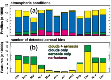
To assess the representativeness of the CALIOP measure-ments in our region of interest around Svalbard, it is worth-while first examining the availability of lidar profiles and the atmospheric conditions (i.e., the abundance of aerosols and clouds) encountered during these observations. Figure 2a shows the number of monthly available lidar profiles sub-divided according to what has been detected in the individ-ual profiles: no features (neither clouds nor aerosols), only aerosols (aerosol features but no cloud features in a profile), only clouds (cloud features but no aerosol features in a pro-file), or clouds and aerosols (both cloud and aerosol features in a profile). For the entire year of 2008, only 5.8 % of the considered 187 711 profiles show conditions of aerosols only (i.e., no disturbance by clouds) that are most favorable for the type of comparison that we pursue in this study. Best con-ditions are found during March (15.1 % cloud-free profiles with aerosols features), while the summer months (May to September), particularly July (0.6 % cloud-free profiles with aerosol features), represent non-ideal conditions for the com-parison of surface measurements and spaceborne observa-tions attempted in this study. About 10 % of all CALIOP pro-files contain neither aerosol nor cloud features with a maxi-mum and minimaxi-mum occurrence rate of 25 and 4 % in July and January, respectively. This effect is due to the weaker signal-to-noise ratio (SNR) of CALIOP measurements during bright daytime conditions (i.e., polar summer) compared to the ab-sence of sunlight during night and the correspondingly higher threshold value that has to be exceeded for feature detection (Winker et al., 2009; Young and Vaughan, 2009). Polar sum-mer and winter can be recognized in the occurrence rate of no features (magenta bars) in Fig. 2a. Observation rates of 50 to 85 % for clouds only (during March and August, respec-tively) illustrate that cloudiness is another main obstacle for deriving aerosol information from CALIOP measurements. Most of these clouds are optically thick and lead to signif-icant or full attenuation of the laser light. As long as these clouds form the uppermost feature, no aerosol detection is possible, even if cloud and aerosol layers are present at dif-ferent height levels.
atmospheric conditions
Profiles (x 1000)
0 5 10 20
15
clouds + aerosols
clouds only aerosols only no features
(
a
)
(
b
)
number of detected aerosol bins
Features (x 10000) 0 2 4 8
6 12 14
10
Figure 2.Histograms of the monthly abundance of(a)CALIOP
level 2 5 km aerosol profiles and(b)60 m height bins with aerosol
observations as detected during 2018 CALIPSO overpasses in the region of interest during 2008. The color coding refers to the ob-served occurrence of atmospheric features (aerosols and/or clouds).
Figure 2b shows the occurrence rate of the number of height bins with aerosol information for profiles that fall into the categories “aerosol only” and “clouds and aerosols” (i.e., profiles identified to contain aerosol information). Note that the information given in Fig. 2a refers to the entire pro-file whereas Fig. 2b refers to the height-resolved observa-tion provided by these profiles. Figure 2b shows that the detection rate of aerosol bins (i.e., the amount of aerosol-containing height bins per profile per month) is much higher during winter, when the background of sunlight is absent and clouds are also less frequent. During summer, almost no aerosol features are detected. This is probably due to the de-creased SNR of the measurement during daytime, the gener-ally cleaner conditions during this time of the year, or a com-bination of both. It is also apparent from Fig. 2b that most aerosol features are detected in combination with clouds in the same profile (yellow) rather than during cloud-free con-ditions (green). Looking at the number of detected aerosol layers given in the CALIPSO products reveals that aerosols occur within a single layer during the majority of observa-tions (not shown). Multiple aerosol layers are only detected during polar night. The observation of two layers is already rare, and the number of cases with four layers is negligible.
summer. Nevertheless, it is worth proceeding with our study for the limited number of available cases in order to assess the value of the combined data sets.
2.4 HYSPLIT trajectories
We use the HYSPLIT (Hybrid Single-Particle Lagrangian In-tegrated Trajectory; Draxler and Rolph, 2010) model of the NOAA Air Resources Laboratory to study the advection of air parcels to and from Zeppelin station. Forward and back-ward trajectories with time intervals of 1 h were calculated starting and arriving every 3 h at the height and location of Zeppelin station, respectively.
Meteorological parameters from the Global Data Assim-ilation System (GDAS) are provided along the trajectories and are used in this study to estimate RH at the location of the CALIPSO overpass.
3 Comparison approach
Anderson et al. (2003) and Kovacs (2006) investigated the regional representativeness of local measurements of atmo-spheric aerosols by correlating these to the distance at which coincident satellite observations were performed. They con-cluded that the distances at which two measurements, both at ambient RH, along a trajectory show acceptable correlation to establish a connection are 300 and 500 km for observations over land and sea sites, respectively. As a result of these ear-lier studies, we considered a region from 0 to 25◦E and from 75 to 82◦N for this study. CALIPSO passed over this area 2018 times in 2008. The closest overpass occurred only 2 km away from Zeppelin station, while the furthest one was at a distance of 360 km.
We started our investigation by applying the closest-approach method to link CALIPSO observations in the re-gion of interest to coincident dry in situ measurements at Zeppelin station. While this course of action led to a high number of matches, it did not enable reasonable case-by-case reconciliation of in situ and remote-sensing data. Differences in the compared aerosol optical properties ranged between 2 and 3 orders of magnitude. Perpetual refinement of the com-parison procedure as described below showed that the failure in reconciling the different observations in the initial com-parison is due to the following:
1. physically meaningless comparison scenarios in which no connection can be established between the locations of the ground site and the satellite track during hetero-geneous aerosol conditions,
2. the inclusion of apparently unrealistic signal spikes in the CALIOP extinction coefficient in the case of fixed or inappropriately selected along-track averaging inter-vals,
3. humidification effects,
4. the temporal delay in the observations.
The first two points make reasonable comparisons impossi-ble. The latter two can still introduce uncertainties of up to 100 %.
Differences in exact location of the measurements pose a severe problem, since the humidity and aerosol content of air is highly variable in time and space (horizontally and verti-cally). Thus, it is essential to select that part of the CALIPSO ground track for which it is most likely that both CALIOP and in situ instrumentation actually sampled the same air mass. Following the approach presented in Tesche et al. (2013), air-mass trajectories are used to connect the in situ station to the segment of the CALIPSO ground track that is most likely to lead to a physically meaningful comparison. The length of the trajectories between Zeppelin station and the intersection with the CALIPSO ground track provides us with the time lag between fitting observations. This trajec-tory matching allows for items 1 and 4 on the list above to be addressed.
Screening of the CALIPSO data is a major effort in obtain-ing meanobtain-ingful comparison cases. Our case-by-case investi-gation shows that profiles fulfilling the quality assurance cri-teria given in Sect. 2.3.1 can still contain data points that are obviously unrealistic and could be due to the low SNR of the observation or improper cloud screening. Though such points have little impact when comparing highly averaged data, they dominate individual comparisons. Here, we selected over-passes that in fact show extinction coefficients (i.e., signals above the CALIOP detection threshold) in a height range from 250 to 730 m that spans around the height of Zeppelin station. This holds for 24 % of all overpasses in the area of interest. Next, we discarded cases for which trajectories start-ing every 3 h at Zeppelin for 15 h after and before an over-pass, respectively, did not cross the CALIPSO ground track. This left 9 % of all 2018 overpasses in 2008. Note that in contrast to Anderson et al. (2003) and Kovacs (2006), who referred to the length scale, we use a timescale and restrict the comparison to a time delay of 15 h. This corresponds to a maximum distance of 360 km at a mean transport velocity of about 7 m s−1. We believe that time rather than distance is a better parameter to assess changes in the aerosol prop-erties in the atmosphere. The majority of the track segments for comparison were located either in the vicinity or to the north (beyond 81◦N) of the ground site (not shown).
individually for each overpass according to the spread of the crossing trajectories with different start times. A change in the along-track average of the CALIOP extinction profile to a fixed interval can result in large differences in the resulting mean extinction profile during heterogeneous conditions or physically meaningless comparison scenarios. Once an ex-tinction profile could be obtained at the proper location for comparison, the values in the height range from 250 to 730 m (eight 60 m height bins) were averaged. We chose this height range to account for vertical motions during the transport from the location of the CALIOP observation to Zeppelin station (backward trajectories) or vice versa (forward trajec-tories). For particular cases, better agreement with the in situ observation may be obtained for an average over a smaller height range. However, we chose a conservative range that was found to be suitable for the majority of cases considered in this study. The average and the corresponding standard deviation (as a measure of vertical homogeneity) represent values used in the comparison to the findings of the mea-surements at Zeppelin station. To coarsely account for uncer-tainties in the trajectories, in situ extinction coefficients were averaged over 5 h (five 1 h values) centered around the time when the in situ instruments sampled the same air parcels as CALIOP, i.e., time of a CALIPSO overpass plus the time lag determined from the length of the trajectories that connect this overpass to Zeppelin station.
4 Results and discussion
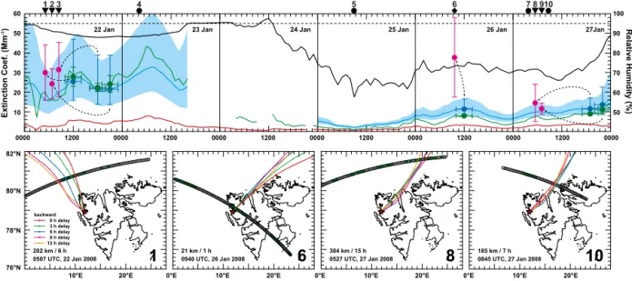
The time period of 22 to 28 January 2008 has been cho-sen to illustrate the analytical work and some of the re-sults obtained. Figure 3 presents the dry scattering coeffi-cient measured with the nephelometer at Zeppelin station and the ambient extinction coefficients derived as described in Sects. 2.2.1 and 2.2.2 during this period. The ambient RH given in the figure reflects the influence of hygroscopicity, which causes the huge differences between dry scattering and ambient extinction values. The latter parameter was not esti-mated when ambient RH exceeded values of 95 %. The time period covered in Fig. 3 shows 10 CALIPSO overpasses that were connected to the ground station with the help of trajec-tories (see symbols and corresponding numbers at the top of Fig. 3). Extinction coefficients extracted from the CALIPSO observations could be compared to ground-based measure-ments for six cases (overpasses 1, 2, 3, 6, 8, and 9). Four ex-amples of how trajectories are used to connect the ground site with the proper segment of the CALIPSO track (overpasses 1, 6, 8, and 10) are given in the lower part of Fig. 3. Tri-angles mark cases for which aerosol profiles were obtained during cloud-free conditions, as indicated by a cloud optical thickness (COT) of zero. The examples of overpasses 1 and 8 show how the trajectories lead to a cloud-free part of the ground track. The different lengths and tracks of the trajecto-ries indicate that time and distance should not be considered
synonymous. The satellite- and ground-based extinction co-efficients agree within their error bars for the overpasses on 22 and 27 January 2008, with the shortest time delay of 6 h (201 km distance) and the longest time delay of 15 h (322 km distance). Note that ambient RH was above 90 % on 22 Jan-uary 2008 and that the difference between the dry scattering coefficient and the RH-corrected extinction coefficient is as much as a factor of 10. A much smaller ratio of ambient to dry extinction coefficients can be found for 26 and 27 Jan-uary 2008, for which RH varies between 65 and 90 %. The cases in Fig. 3 illustrate the importance of accounting for the proper time delay between the measurements of CALIOP and in situ instrumentation. Using the in situ measurements at the time of the satellite overpass increases the ratio of the ambient extinction coefficients from in situ and CALIOP ob-servations by 30 % for the example cases in Fig. 3.
Using the trajectories as described above, a cloudy part of the CALIPSO ground track (COT>0, AOT=0) was
identi-fied for the overpasses 4, 5, 7, and 10. No comparisons could be performed since there is no aerosol information available for these cases. This kind of situation inhibited comparisons in 127 cases for the months January to April and October to December 2008. Typical scenarios are as follows: no height bins are marked as containing aerosols at all, all aerosols are located above or below our height range of interest, or the ob-tained aerosols profile is of unreasonable shape and/or mag-nitude.
For overpass 6 in Fig. 3, aerosol information was obtained in cloudy environment (COT>0, AOT>0). Even though
this overpass occurred only 21 km from the ground site, the CALIPSO observation is in disagreement with the result of the in situ measurement. This emphasizes that using a closest approach for comparison of ground-based measurements and CALIPSO observations might not always be the best choice. The case also illustrates that even few clouds can disturb aerosol measurements with spaceborne lidar. Note also that trajectories might actually lead to a track segment that is not closest to the ground site, as is the case for overpass 8.
50 60 70 80 90 100
10 20 30 40 50 60
22 Jan
0000 1200
23 Jan
0000 1200
24 Jan
0000 1200
25 Jan
0000 1200
26 Jan
0000 1200
27Jan
0000 1200 0000
76°N 78°N 80°N 82°N
10°E 20°E 0°E 10°E 20°E 0°E 10°E 20°E 0°E 10°E 20°E
Extinction Coef. (Mm
-1)
Relative Humidity (%)
0507 UTC, 22 Jan 2008 0 h delay backward
3 h delay 6 h delay 9 h delay 12 h delay 202 km / 6 h
1 2 3 4 5 6 7 8 910
1
0527 UTC, 27 Jan 2008304 km / 15 h
8
0845 UTC, 27 Jan 200810
185 km / 7 h0940 UTC, 26 Jan 2008 21 km / 1 h
6
Figure 3.Upper panel: CALIPSO extinction coefficient (532 nm, magenta circles) compared to in situ measurements of the dry scattering
coefficient (550 nm, red line) and the ambient extinction coefficient determined from the measurements of DMPS (550 nm, green line) and nephelometer plus PSAP (550 nm, blue line) for the time period of 22 to 27 January 2008. The blue shaded area marks the region of possible values based on the minimum and maximum estimates of theγ value. Green and blue circles mark 5 h averages of the ambient extinction
coefficients from the in situ observations. Arrows show which values are compared. Ambient RH is given in black. Values above RH>95 %
were disregarded (dashed black line). Symbols and corresponding numbers mark CALIPSO overpasses that could be connected to the ground site for the considered time period: only aerosol features (triangles), aerosol and cloud features (diamond), and no or only cloud features (circles). Lower panel: presentation of the use of trajectories to connect the in situ site to the spaceborne measurements for four selected cases (marked as 1, 6, 8, and 10 in the upper plot). The CALIPSO ground track is marked by gray (no aerosol data available) and green (aerosol data available) circles, which refer to individual 5 km aerosol profiles. Colored dots and lines mark backward trajectories starting close to the CALIPSO overpass (red) as well as 3 h (green), 6 h (blue), 9 h (magenta), and 12 h (orange) after the overpass. The time of overpass is given in the respective plots. The red star marks the location of Zeppelin station.
range rather than time for comparison. This suggests that the method of comparing local point or column-integrated mea-surements to the closest-approach observation of CALIPSO is likely to yield misleading results.
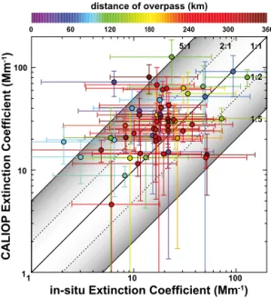
We performed a deeper analysis of the factors that could explain why a difference of as large as a factor of 5 occurs for some of the cases included here. Besides the spatial distance and temporal delay between the observations, we considered the relative humidity at Zeppelin station and at the crossing point of the satellite ground track and trajectories, the occur-rence of clouds and rain along the trajectory, and the wind direction at the ground site. However, only the latter param-eter could be linked to the outliers in Fig. 4. Figure 5a shows that the largest absolute difference in the ambient extinction coefficients from CALIOP and in situ measurements occurs during westerly flow. It could be that aerosol conditions are more stable for air masses approaching Zeppelin station from the north and via ice-covered ocean compared to the open water to the west. On the other hand, the CALIOP aerosol classification scheme can choose from a larger pool of li-dar ratios for observations over ocean and land compared to those over snow and ice (Omar et al., 2009). Hence, we inves-tigated the dominant aerosol type selected in the CALIPSO data retrieval for the individual comparisons. It was found
that the most characteristic outliers in Figs. 4 and 5a occur for cases that were identified predominantly as polluted dust or polluted continental. These aerosol types are rather uncom-mon at 78◦N and suggest misclassification in the CALIPSO retrieval. Misclassification can occur as a result of signal noise, improper cloud screening, or due to surface effects. Given the structure of the CALIPSO aerosol classification scheme described in Omar et al. (2009), CALIOP observa-tions in the Svalbard region during background condiobserva-tions (weakly depolarizing and integrated attenuated backscatter coefficient not exceeding the threshold value of 0.0015 at 532 nm) should be classified as clean continental (over land and snow/ice) and clean marine (over ocean).
1
360 300 240 0 60 120 180
1
10 10
100 100
CALIOP
Extinction Coefficient (Mm
-1)
in-situ Extinction Coefficient (Mm-1)
distance of overpass (km)
1:1 5:1 2:1
1:2
1:5
Figure 4.Comparison of the ambient 550 nm extinction coefficient
from humidification of nephelometer and PSAP measurements (see Sect. 2.2.2) vs. the ambient 532 nm extinction coefficient extracted from CALIPSO overpasses for 57 suitable cases. The color coding describes the distance of the CALIPSO observation from the ground site. Error bars refer to the results of using the lower and upper estimate in theγvalue for humidification and the standard deviation
from averaging over nine 60 m CALIPSO height bins between 250 and 730 m, respectively. Ratios of 1 : 1, 1 : 2, and 1 : 5 are marked by solid and dashed lines and the shaded area.
Strong variation in RH between the location of the CALIPSO ground track and Zeppelin station could also cause the scatter of values presented in Fig. 4. Such RH dif-ferences have a direct effect on the scattering enhancement factorf(RH) and thus the difference between dry and
ambi-ent extinction coefficiambi-ents. The scattering enhancemambi-ent fac-tor was found to be much higher for Arctic aerosol compared to observations at continental, background, or marine sites (Zieger et al., 2013). Consequently, we should expect that even small differences in RH between the measurements at Zeppelin and along the satellite track can lead to high differ-ences in the ambient extinction coefficient. This holds espe-cially for high RH>85%. We investigated whether we can
find a connection between the difference in RH (1RH) at the
two measurement locations (i.e., the CALIOP ground-track segment and Zeppelin station) and the agreement in the com-parison of ambient extinction coefficients at those sites. The RH at the location of the CALIOP observation is taken from the meteorological data provided with the trajectory analy-sis and is thus highly uncertain. For the 57 cases considered, the1RH showed a mean value of 12±10 % (mean RH of
80±12 % at Zeppelin station) with a maximum value of
around 30 % (not shown). Though 1RH was considerable
for several cases, we could not establish whether this factor or the resulting difference in f (RH)can fully explain the
-60 -40 -20 0 20 40 60 80 100
Abs. Diff. in Extinction Coefficient (Mm-1)
0.0 0.5 1.0
Normalized Rel. Diff. in Extinction Coefficient
Figure 5.Detailed view of(a)the effect of wind direction on the
ab-solute difference in the ambient extinction coefficients derived from observations at Zeppelin and by CALIOP and(b)the connection
between the relative difference1f (RH)of the scattering
enhance-ment factors at Zeppelin station and at the intersection of trajecto-ries and CALIPSO ground track and the relative difference in the ambient extinction coefficients observed at the two locations. The color coding refers to the dominant aerosol type identified in the CALIOP observations (cm – clean marine; d – dust; pc – polluted continental; cc – clean continental; pd – polluted dust; s – smoke, not observed) and the difference in RH observed at Zeppelin sta-tion and taken from the trajectory calculasta-tions at the locasta-tion of the CALIPSO overpass, respectively. The dashed line marks the 1 : 1 line.
disagreement found in the ambient extinction coefficients. Figure 5b shows the connection between the relative differ-ence inf (RH)at the locations of CALIOP and in situ
ob-servations and the relative difference in the ambient extinc-tion coefficients obtained from these observaextinc-tions. If hygro-scopic growth were the only factor necessary to consider in our comparison, values should align along the 1 : 1 line. De-viations are likely to be related to the observation of different air masses at the two locations or the improper representation of meteorological parameters in the trajectory model.
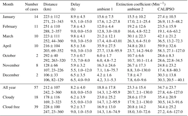
Table 1 gives a detailed overview of the results obtained from the comparison of spaceborne and ground-based ob-servations subdivided according to the months of 2008 and whether cloud-free or cloudy CALIOP aerosol profiles were used in the comparison. For the 57 considered cases, Table 1 shows that time delay is rather evenly distributed between 0 and 15 h with a median of 8 h. Of the 57 suitable cases, 39 oc-curred during most favorable cloud-free conditions (AOT>
Table 1.Results of the comparison of CALIPSO observations and in situ measurements at Zeppelin station (ambient 1 and 2 as in Fig. 1)
subdivided according to months of the year 2008 and cloud-free and cloudy conditions in the CALIPSO aerosol profiles. The first line (columns 3–7) refers to mean values and standard deviation, while the second line refers to median and range of values.
Month Number Distance Delay Extinction coefficient (Mm−1)
of cases (km) (h) ambient 1 ambient 2 CALIPSO
January 14 223±112 8.9±4.5 15.6±7.5 15.5±10.2 27.4±10.5
271, 21–343 9.5, 1.0–15.0 17.6, 1.2–27.8 17.0, 2.1–25.4 26.9, 11.5–48.2
February 11 251±110 7.8±4.3 12.0±4.4 19.2±12.6 23.5±15.9
288, 2–357 9.0, 0.0–15.0 12.8, 3.0–18.0 16.6, 4.8–52.2 19.1, 4.6–63.2
March 10 223±111 9.8±4.1 21.2±12.1 30.1±22.3 42.1±21.2
252, 44–360 9.0, 3.0–15.0 17.4, 4.0–43.01 26.3, 6.4–51.0 36.5, 13.2–72.3
April 10 216±104 8.5±3.6 35.9±27.5 34.8±20.1 59.9±32.6
203, 69–352 9.0, 3.0–13.0 27.7, 13.8–95.9 23.7, 14.2–94.0 58.3, 27.1–127.0
October 2 292±40 7.5±0.7 6.0±1.7 10.7±6.6 28.6±8.3
292, 263–320 7.5, 7.0–8.0 6.0, 4.8–7.2 10.7, 10.1–11.4 28.6, 22.8–34.5
November 8 128±66 5.9±3.2 16.3±24.6 26.7±17.3 24.8±23.2
107, 23–226 5.5, 1.0–12.0 7.1, 1.6–75.7 8.8, 3.0–130.0 17.4, 8.8–80.3
December 2 106±33 6.5±3.5 4.2±1.6 7.8±4.7 30.3±13.8
106, 82–129 6.5, 4.0–9.0 4.2, 3.1–5.3 7.8, 6.0–9.6 30.3, 20.5 – 40.1
All year 57 212±107 8.2±4.0 18.8±17.8 23.3±15.4 34.7±23.7
242, 2–360 8.0, 0.0–15.0 14.3, 1.2–95.9 20.7, 2.1–130.0 27.8, 4.6–127.0
Cloudy 18 178±116 6.2±3.9 23.0±25.2 28.6±17.9 35.4±20.9
169, 2–323 5.5, 0.0–13.0 14.7, 1.2–95.9 17.9, 2.1–130.0 30.5, 14.3–91.6
Cloud free 39 228±100 9.2±3.7 16.9±13.0 20.8±14.2 34.4±25.2
247, 23–360 9.0, 1.0–15.0 14.3, 1.6–74.9 18.0, 3.0–72.6 27.2, 4.6–127.0
comparisons (AOT>0, COT>0). Resolving the
compari-son according to cloudiness in the CALIPSO observations (not shown) leads to ambiguous results: for 7 of the 18 cloudy cases (39 %) a difference larger than a factor of 2 is found between the extinction coefficients from CALIOP and Zeppelin station, while for the cloud-free cases 17 out of 39 (44 %) exceed this difference. The average time delay is 9.2±3.8 h for cloud-free cases, while it is only 6.2±3.9 h
for cloudy cases. Accordingly, cloud-free cases show a mean distance of 228±100 km and cloudy ones 178±116 km.
Extinction coefficients from CALIPSO vary between 4.6 and 127.0 Mm−1for cloud-free cases, while the range of values
for cloudy profiles is much narrower and only spans from 14.3 to 91.6 Mm−1.
5 Summary and conclusions
This study presents a comparison of extinction coefficients as determined from spaceborne lidar (CALIOP) measurements and from ground-based in situ measurements at Zeppelin sta-tion, Ny-Ålesund, Svalbard, during the year 2008. To obtain meaningful comparison, we had to consider several issues:
1. Neither in situ instruments nor spaceborne lidar (CALIOP) provide us with direct measurements of the ambient aerosol extinction coefficient.
2. Approved methods were used to obtain ambient extinc-tion coefficients from dry in situ measurements per-formed with commonly used instruments.
3. Extinction coefficients from the spaceborne sensor were taken from operational CALIPSO products that under-went elaborate calibration and quality assurance. 4. Air-mass trajectories were used to ensure that
compar-isons were performed for the same air mass. They al-low a connection to be established between the satel-lite’s ground track and Zeppelin station and the along-track averaging intervals to be adapted according to the spatial spread of the crossing trajectories. The averag-ing height range of 510 m centered at the elevation of the ground site was chosen to account for vertical dis-placement during travel along the trajectories. Temporal averaging of ground-based data of 5 h further mitigates imprecision in the trajectory output.
hours were applied in this study, we cannot draw conclusions about what will happen if the length of the temporal averag-ing window is increased. The median ambient extinction co-efficient for the 57 comparison cases was 27.8 Mm−1for the
CALIOP data compared to values of 14.3 and 20.7 Mm−1
derived from in situ measurements of the particle size distri-bution and dry scattering coefficients, respectively. The dif-ferent humidity during the measurement in the atmosphere and within a laboratory is an ever-present limitation for stud-ies like the one presented here. The thermodynamic state (e.g., RH) of the samples and the assumptions on the hygro-scopic properties for the in situ measurements are therefore vital factors for a successful comparison of aerosol extinc-tion coefficients. In the case of our study, results are also in-fluenced by the CALIPSO aerosol model that is required for the extinction-coefficient retrieval, the CALIOP feature de-tection limit, and the criteria that are used to match satellite observations to the measurement at the ground site.
Detailed knowledge of the humidity field is of vital im-portance when relating in situ measurements to observa-tions with spaceborne sensors. The effect of relative humid-ity on the light-scattering properties of aerosol particles in the atmosphere is the dominant obstacle for a systematic reconciliation of measurements of the two platforms. Ad-ditional problematic factors in the allocation procedure ap-plied in this study were unfavorable wind direction (no in-tersection between trajectories and ground track), presence of clouds (RH>95 % at Zeppelin station and/or no aerosol
information from CALIOP), no data from Zeppelin station or CALIOP, and the CALIOP detection threshold that pre-vents reliable aerosol detection in the presence of sunlight. CALIOP detects almost no aerosol features in the Svalbard region during Arctic summer even though the tropospheric median AOT is generally larger than 0.05 at visible wave-lengths during May and June (Tomasi et al., 2007, 2012; Glantz et al., 2014). This is in agreement with the study by Di Pierro et al. (2013), which investigated the distribu-tion of aerosols in the Arctic from CALIOP measurements. Consequently, CALIOP data have to be treated with great caution when they are used for studies of aerosol occur-rence rate, transport patterns, radiative effects, and interac-tions with clouds under background condiinterac-tions during polar day.
Based on the study presented here we also conclude that consolidating data sets that are averaged over large areas and/or long time periods can lure us into a sense of false confidence, whereas in fact there may actually be weak or no connection between individual observations. Using highly averaged parameters in the deduction of scientific findings is of particular importance for the validation of model simula-tions. Consequently, special emphasis should be placed on proper selection of temporal and spatial averaging intervals when attempting to use spaceborne lidar observations in con-nection with ground-based measurements and model outputs.
Acknowledgements. CALIOP data used in this study were obtained
from the NASA Langley Research Center Atmospheric Science Data Center (http://eosweb.larc.nasa.gov). We thank Birgitta Noone and Tabea Hennig for maintaining the in situ instruments at Zep-pelin station. The Swedish Environmental Agency and Stockholm University are acknowledged for long-term support of the observa-tions at Zeppelin station. We also acknowledge the support within CLIMSLIP. Paul Zieger was supported by a postdoc fellowship of the Swiss National Science Foundation (grant no. P300P2_147776).
Edited by: A. Petzold
References
Anderson, T. and Ogren, J.: Determining aerosol radiative proper-ties using the TSI 3563 integrating nephelometer, Aerosol Sci. Tech., 29, 57–96, 1998.
Anderson, T. L., Charlson, R. J., Winker, D. M., Ogren, J. A., and Holmén, K.: Mesoscale variations of tropospheric Aerosols, J. Atmos. Sci., 60, 119–136, 2003.
CALIPSO Users Guide (2012), Lidar Level 2 5 km
Cloud and Aerosol Profile Products, available at: http://www-calipso.larc.nasa.gov/resources/calipso_users_ guide/data_sum-maries/profile_data.php, last access: 6 February 2014.
Covert, D. S. and Heintzenberg, J.: Size distributions and chemical properties of aerosol at Ny-Ålesund, Svalbard, Atmos. Environ., 27, 2989–2997, 1993.
Di Pierro, M., Jaeglé, L., Eloranta, E. W., and Sharma, S.: Spa-tial and seasonal distribution of Arctic aerosols observed by the CALIOP satellite instrument (2006–2012), Atmos. Chem. Phys., 13, 7075–7095, doi:10.5194/acp-13-7075-2013, 2013.
Draxler, R. R. and Rolph, G. D.: HYSPLIT (HYbrid Single-Particle Lagrangian Integrated Trajectory) Model access via NOAA ARL READY Website (http://ready.arl.noaa.gov/HYSPLIT. php), NOAA Air Resources Laboratory, Silver Spring, MD, 2010.
Eleftheriadis, K., Vratolis, S., and Nyeki, S.: Aerosol black car-bon in the European Arctic: Measurements at Zeppelin station, Ny-Ålesund,Svalbard from 1998–2007, Geophys. Res. Lett., 36, L02809, doi:10.1029/2008GL035741, 2009.
Eneroth, K., Kjellström, E., and Holmén, K.: A trajectory clima-tology for Svalbard; investigating how atmospheric flow patterns influence observed tracer concentrations, Phys. Chem. Earth, 28, 1191–1203, doi:10.1016/j.pce.2003.08.051, 2003.
Glantz, P., Bourassa, A. E., Herber, A., Iversen, T., Karlsson, J., Kirkevåg, A., Maturilli, M., Seland, Ø., Stebel, K., Struthers, H., Tesche, M., and Thomason, L.: Remote sensing of aerosols in the Arctic for an evaluation of global climate model simulations, J. Geophys. Res., 119, 8169–8188, doi:10.1002/2013JD021279, 2014.
Herber, A., Thomason, L. W., Gernandt, H., Leiterer, U., Nagel, D., Schulz, K.-H., Kaptur, J., Albrecht, T., and Notholt, J.: Continu-ous day and night aerosol optical depth observations in the Arctic between 1991 and 1999, J. Geophys. Res., 107, AAC 6-1–ACC 6-13, doi:10.1029/2001JD000536, 2002.
aerosol experiments in southern Ontario, J. Geophys. Res., 101, 19199–19209, doi:10.1029/95JD03228, 1996.
Hoffmann, A., Ritter, C., Stock, M., Shiobara, M., Lampert, A., Ma-turilli, M., Orgis, T., Neuber, R., and Herber, A.: Ground-based lidar measurements from Ny-Ålesund during ASTAR 2007, At-mos. Chem. Phys., 9, 9059–9081, doi:10.5194/acp-9-9059-2009, 2009.
Hoffmann, A., Osterloh, L., Stone, R., Lampert, A., Ritter, C., Stock, M., Tunved, P., Hennig, T., Böckmann, C., Li, S.-M., Eleftheriadis, K., Maturilli, M., Orgis, T., Herber, A., Neuber, R., and Dethloff, K.: Remote sensing and in-situ measurements of tropospheric aerosol, a PAMARCMiP case study, Atmos. En-viron., 52, 56–66, doi:10.1016/j.atmosenv.2011.11.027, 2012. Kovacs, T.: Comparing MODIS and AERONET aerosol optical
depth at varying separation distances to assess ground-based val-idation strategies for spaceborne lidar, J. Geophys. Res., 111, D24203, doi:10.1029/2006JD007349, 2006.
Kreidenweis, S. M., Koehler, K., DeMott, P. J., Prenni, A. J., Carrico, C., and Ervens, B.: Water activity and activation di-ameters from hygroscopicity data – Part I: Theory and appli-cation to inorganic salts, Atmos. Chem. Phys., 5, 1357–1370, doi:10.5194/acp-5-1357-2005, 2005.
Mauritsen, T., Sedlar, J., Tjernström, M., Leck, C., Martin, M., Shupe, M., Sjogren, S., Sierau, B., Persson, P. O. G., Brooks, I. M., and Swietlicki, E.: An Arctic CCN-limited cloud-aerosol regime, Atmos. Chem. Phys., 11, 165–173, doi:10.5194/acp-11-165-2011, 2011.
Masonis, S., Ansmann, A., Müller, D., Althausen, D., Ogren, J. A., Jefferson, A., and Sheridan, P. J.: An intercomparison of aerosol light extinction and 180◦ backscatter as derived
us-ing in situ instruments and Raman lidar durus-ing the INDOEX field campaign, J. Geophs. Res., 107, INX2 13-1–INX2 13-21, doi:10.1029/2000JD000035, 2002.
Müller, D., Ansmann, A., Mattis, I., Tesche, M., Wandinger, U., Althausen, D., and Pisani, G.: Aerosol-type-dependent lidar ra-tios observed with Raman lidar, J. Geophys. Res., 112, D16202, doi:10.1029/2006JD008292, 2007.
Omar, A. H., Winker, D. M., Vaughan, M. A., Hu, Y., Trepte, C. R., Ferrare, R. A., Lee, K.-P., and Hostetler, C. A.: The CALIPSO automated aerosol classification and lidar ratio se-lection algorithm, J. Atmos. Ocean. Tech., 26, 1994–2014, doi:10.1175/2009JTECHA1231.1, 2009.
Petters, M. D. and Kreidenweis, S. M.: A single parameter repre-sentation of hygroscopic growth and cloud condensation nucleus activity, Atmos. Chem. Phys., 7, 1961–1971, doi:10.5194/acp-7-1961-2007, 2007.
Rastak, N., Silvergren, S., Zieger, P., Wideqvist, U., Ström, J., Svenningsson, B., Maturilli, M., Tesche, M., Ekman, A. M. L., Tunved, P., and Riipinen, I.: Seasonal variation of aerosol water uptake and its impact on the direct radiative effect at Ny-Ålesund, Svalbard, Atmos. Chem. Phys., 14, 7445–7460, doi:10.5194/acp-14-7445-2014, 2014.
Skupin, A., Ansmann, A., Engelmann, R., Baars, H., and Müller, T.: The Spectral Aerosol Extinction Monitoring System (SAE’MS): setup, observational products, and comparisons, Atmos. Meas. Tech., 7, 701–712, doi:10.5194/amt-7-701-2014, 2014. Stock, M., Ritter, C., Herber, A., von Hoyningen-Huene, W.,
Baibakov, K., Gräser, J., Orgis, T., Treffeisen, R., Zinoviev, N., Makshtas, A., and Dethloff, K.: Springtime Arctic aerosol:
Smoke versus haze, a case study for March 2008, Atmos. Envi-ron., 52, 48–55, doi:10.1016/j.atmosenv.2011.06.051, 2012. Stock, M., Ritter, C., Aaltonen, V., Aas, W., Handorff, D., Herber,
A., Treffeisen, R., and Dethloff, K.: Where does the optically detectable aerosol in the European Arctic come from?, Tellus B, 66, 21450, doi:10.3402/tellusb.v66.21450, 2014.
Ström, J., Umegård, J., Tørseth, K., Tunved, P., Hansson, H.-C., Holmén, K., Wismann, V., Herber, A., and König-Langlo, G.: One year of particle size distribution and aerosol chemi-cal composition measurements at the Zeppelin station, Svalbard, March 2000 – March 2001, Phys. Chem. Earth, 28, 1181–1190, doi:10.1016/j.pce.2003.08.058, 2003.
Tang, I. N. and Munkelwitz, R. H.: Aerosol Phase Transformation and Growth in the Atmosphere, J. Appl. Meteorol., 33, 791–796, 1994.
Tang, I. N.:, Chemical and size effects of hygroscopic aerosols on light scattering coefficients, J. Geophys. Res., 101, 19245– 19250, doi:10.1029/96JD03003, 1996.
Tesche, M., Wandinger, U., Ansmann, A., Müller, D., Althausen, D., and Omar, A. H.: Ground-based validation of CALIPSO ob-servations of dust and smoke in the Cape Verde region, J. Geo-phys. Res., 118, 2889–2902, doi:10.1002/jgrd.50248, 2013. Tomasi, C., Vitale, V., Lupi, A., Di Carmine, C., Campanelli, M.,
Herber, A., Treffeisen, R., Stone, R. S., Andrews, E., Sharma, S., Radionov, V., von Hoyningen-Huene, W., Stebel, K., Hansen, G. H., Myhre, C. L., Wehrli, C., Aaltonen, V., Lihavainen, H., Virkkula, A., Hillamo, R., Ström, J., Toledano, C., Ca-chorro, V. E., Ortiz, P., de Frutos, A. M., Blindheim, S., Frioud, M., Gausa, M., Zielinski, T., Petelski, T., and Yamanouchi, T.: Aerosols in polar regions: A historical overview based on optical depth and in situ observations, J. Geophys. Res., 112, D16205, doi:10.1029/2007JD008432, 2007.
Tomasi C., Lupi, A., Mazzola, M., Stone, R. S., Dutton, E. G., Her-ber, A., Radionov, V. F., Holben, B. N., Sorokin, M. G., Sak-erin, S. M., Terpugova, S. A., Sobolewski, P. S., Lanconelli, C., Petkov, B. H., Busetto, M., and Vitale, V.: An update on polar aerosol optical properties using POLAR-AOD and other mea-surements performed during the International Polar Year, Atmos. Environ., 52, 29–47, doi:10.1016/j.atmosenv.2012.02.055, 2012. Tunved, P., Ström, J., and Krejci, R.: Arctic aerosol life cycle: link-ing aerosol size distributions observed between 2000 and 2010 with air mass transport and precipitation at Zeppelin station, Ny-Ålesund, Svalbard, Atmos. Chem. Phys., 13, 3643–3660, doi:10.5194/acp-13-3643-2013, 2013.
Winker, D. M., Vaughan, M. A., Omar, A. H., Hu, Y., Pow-ell, K. A., Liu, Z., Hunt, W. H., and Young, S. A.: Overview of the CALIPSO mission and CALIOP data pro-cessing algorithms, J. Atmos. Ocean. Tech., 26, 2310–2323, doi:10.1175/2009JTECHA1281.1, 2009.
World Meteorological Organization: Aerosol measurement proce-dures guidelines and recommendations, GAW Report No. 153, World Meteorological Organization Global Atmosphere Watch, Geneva, Switzerland, 2003.
Zieger, P., Fierz-Schmidhauser, R., Gysel, M., Ström, J., Henne, S., Yttri, K. E., Baltensperger, U., and Weingartner, E.: Effects of relative humidity on aerosol light scattering in the Arctic, Atmos. Chem. Phys., 10, 3875–3890, doi:10.5194/acp-10-3875-2010, 2010.
Zieger, P., Weingartner, E., Henzing, J., Moerman, M., de Leeuw, G., Mikkilä, J., Ehn, M., Petäjä, T., Clémer, K., van Roozen-dael, M., Yilmaz, S., Frieß, U., Irie, H., Wagner, T., Shaigan-far, R., Beirle, S., Apituley, A., Wilson, K., and Baltensperger, U.: Comparison of ambient aerosol extinction coefficients ob-tained from in-situ, MAX-DOAS and LIDAR measurements at Cabauw, Atmos. Chem. Phys., 11, 2603–2624, doi:10.5194/acp-11-2603-2011, 2011.
Zieger, P., Kienast-Sjögren, E., Starace, M., von Bismarck, J., Bukowiecki, N., Baltensperger, U., Wienhold, F. G., Peter, T., Ruhtz, T., Collaud Coen, M., Vuilleumier, L., Maier, O., Emili, E., Popp, C., and Weingartner, E.: Spatial variation of aerosol optical properties around the high-alpine site Jungfraujoch (3580 m a.s.l.), Atmos. Chem. Phys., 12, 7231–7249, doi:10.5194/acp-12-7231-2012, 2012.