w w w . a j e r . o r g Page 98
American Journal of Engineering Research (AJER)
e-ISSN : 2320-0847 p-ISSN : 2320-0936
Volume-03, Issue-04, pp-98-107
www.ajer.org
Research Paper Open Access
Variation of Stress Range Due to Variation in Sea States
–
An
Overview of Simplified Method of Fatigue Analysis of Fixed
Jacket Offshore Structure
1
Aliyu Baba,
2Musa Aliyu Dahiru
1
(Department of Civil Engineering, Modibbo Adama University of Technology Yola, Adamawa State, Nigeria) 2
(Department of Civil Engineering, Modibbo Adama University of Technology Yola, Adamawa State, Nigeria)
Abstract: - In this paper the simplified method of fatigue analysis of fixed offshore structure was considered. For the purpose of this study,the model was analyzed using ANSYS, and by progressively stepping the regular wave through the structure, a range of stress, S, was identified for each critical point on the structure as the nominal stress range, which was then multiplied by SCF of 1.07 to obtain the actual stress range for six different sea states for time intervals, t = 0, T/4, T/2, 3T/4 and T.
Keywords: - Fatigue Analysis, Fixed Jacket Structure, Stress Range, S-N Curve
I. INTRODUCTION
Offshore structures of all types are generally subjected to cyclic loading from wind, current, earth-quakes and waves acting simultaneously, which cause time-varying stresses in the structure. The environmental quantities are of a random nature and are more or less correlated to each other through the generating and driving mechanism. Offshore structures, regardless of location, are subject to fatigue degradation. In many areas, fatigue is a major design consideration due to relatively high ratios of operational sea states to maximum design environmental events [1].
The simplified fatigue analysis is also called allowable stress range method. This method is based on the premise that it is possible to evaluate a long term stress range and compare its maximum value with the allowable stress limit. For this reason the simplified method is classified as an indirect method, as it is not necessary to obtain the fatigue life and damage for each point of the structure in order to perform a fatigue design check [2].
1.1 An Overview of Fatigue in Offshore Structures
Generally speaking, fatigue is the gradual deterioration of materials and welded connections when subjected to cyclic stresses caused by variable loads experienced by the structure during its life, and accounts for about 90% of failures in welded structures. Failure can occur due to repeated loads (even) below the static yield strength, and can result in an unexpected and catastrophic failure in use if these connections are not designed to resist the fatigue damage. Locations in the structure most prone to fatigue are:
Intersection of tubular members because of Hot Spot stresses
Hatch corners in ship decks
Deck house endings
Tank boundaries due to sloshing of liquids, and
Structural connections, especially where weld details are poor
Fatigue under random loading conditions experienced offshore is a complex subject and the following comments are accepted to be true for welded steel structures [3].
w w w . a j e r . o r g Page 99
Small sharp defects inevitably exist in welds and act as crack initiators; hence fatigue in offshore structures is predominantly a matter of crack propagation.
In as welded connections, stresses of yield strength magnitude in tension exist due to residual stresses.
Stress fluctuations are therefore, from tension yield downwards and the range of the fluctuation only is the governing parameter.
In welded structures fully tensile stress cycles and wholly or partially compressive stress cycles are equally damaging.
The fatigue strength of welded connections is independent of the yield strength of the currently used structural steels.
Crack propagation and consequently fatigue damage in an offshore environment will continue at some range , that is there is no endurance limit as is found above 2x10⁶ cycles, and
Shear stress may be neglected in fatigue life calculations.
In offshore structures, stress fluctuations due to variable loading occur predominantly as a result of wave loads. Studies indicate that fatigue in offshore structures is a typical high cycle phenomenon. Most damage, by far, is caused by the occurrence of many cycles of stress ranges. The occurrence of a few exceptionally severe storms, with return periods of more than one year is unimportant in fatigue damage considerations. Consequently the response of structure in sea states of relatively low wave height and short mean wave period is of prime concern.
Steel jacket structures commonly used for exploration and production of oil and gas composed of steel tubular members, which are interconnected by welded joints. The joints may cause large stress concentrations, which severely affect the fatigue life. For offshore structures, which are subjected to considerable dynamic loading from waves, fatigue is in many cases a dominating design criterion [4].
The subject of fatigue in structures is very broad and varied. So many papers, reports and books have been written on the subject, although most of the material is highly specialized and not readily available to the general public. Detailed history of fatigue which started in the early 19th century as a by-product of the industrial revolution can be found in[5].
The vast amount of literature on the subject testifies to the fact that numerous research programs were carried out on it in the past. The research was stimulated by the need for information on designing against fatigue as well as by the scientific interest to understand the phenomenon of fatigue. An important stimulus for fatigue research also came from catastrophic accidents due to fatigue problems [5].
Many different approaches are available for analyzing offshore jacket platforms in order to compute the fatigue life of the structure. The correct choice of approach depends on a number of factors, such as whether the structure is linear or nonlinear, or whether dynamic response is significant or not. In general, there are three methods for the determination of fatigue damage: the Spectral Method, the Deterministic Method, and the Simplified Method.
II. METHODOLOGY AND MATERIALS
In this study, Simplified method was chosen to determine the fatigue life of the jacket structure as the jacket will be operating in a shallow water (27.8m depth) and, the Simplified method of approach is often undertaken for shallow water (statically responsive) structures subject to some nonlinearities [6].
With this method, the fatigue damage caused by the representative set of regular waves is used, along with the probability of occurrence (See TABLES I & III) for each regular wave, to find the fatigue life of the
structure. Each wave was separately applied to the structure. A wave loading analysis, incorporating Morrison’s
loading calculation and the linear (Airy) wave theory.
The jacket was model in ANSYS and part of the structure under water was discretized in to (264) Beam elements. The material type used was BEAM4 (3D) which is a uniaxial element with tension, compression, torsion, and bending capabilities. The element has six degrees of freedom at each node: translations in the nodal x, y, and z directions and rotations about the nodal x, y, and z axes. Stress stiffening and large deflection capabilities are also included. The part of the structure under water was divided in to 32 members (See Fig. 8 as one of the model sample) and all the loads were computed based on the number of these members. All the members were then subdivided in to elements and the loads were applied on the elements at the nodes as pressure on beam and for each element, i, stands for pressure at first node and j, stands for pressure at second node while the loads from the super structure were applied as point loads at the node (top) of each vertical member.
w w w . a j e r . o r g Page 100
Based on this stress range, the allowable number of cycles to failure, N, for this given stress level was obtained from the appropriate (S – N) fatigue strength curve. The S – N curve (Fig. 1) [8] contains three curves thus, for tubular joints in Air (A), in sea water with cathodic protection (CP), and in sea water for free corrosion (FC) but the former was neglected because of the consideration of only part of the structure under water. Therefore, values of N for the two curves (i.e. NCP and NFC) was then computed and sum up together to get the total number of cycle to failure which was then compared with n, the actual number of waves (equivalent to cycles), which would be available from environmental measurements in order to compute the fatigue damage increment. This was repeated for the other wave heights in order to accumulate the fatigue damage for all the sea wave conditions thus,
=
�
=1 “equation 1"
Where is the number of cycles the structural detail endures at stress range , � is the number of cycles to failure at stress range , as determined by the appropriate S-N curve, and j is the number of considered stress range intervals. Hence the fatigue life was evaluated from;
= 1 “equation 2” where = fatigue life in years, = fatigue damage
The fatigue life of the jacket structure then computed based on the stress range obtained from the previous tables by multiplying the stresses by a stress concentration factor of 1.07 [8]to get the number of cycles to failure N from the S-N Curve. The number of cycles per year n can also be computed from the data in the wave scatter table of global statistics of area 58 in West Africa. Table III, presents the summary of the probability of occurrences in the data available from the environmental measurements.
III. MATHEMATICAL DEVELOPMENT
The long term stress range distribution may be presented as a two parameter weibull distribution;
Fs(S) = exp − S > 0 “equation 3”
Where;
Fs(S) = is the probability that the value S will be exceeded
S = is the random variable representing the stress range
Γ = is the weibull shape factor δ = is the weibull scale factor
This equation is used in the simplified fatigue analysis, which is based on the cumulative damage rule (Palmgren-Miner), taking in to account also the fatigue strength defined by S-N curves. A closed expression for the fatigue damage can be found, based on it.
The weibull distribution parameters are given below:
Let SR = a reference stress range be the major stress range that can occur on a certain number NR of cycles.
δ = � 1
“equation 4”
3.1 Fatigue Damage
It can be shown that the closed solution for the fatigue damage considering a two segment S-N curve is as given below:
D = � .
� .Г + 1,� +
� .
.Г0 �+ 1,�
“equation 5”
Where;
NT = the total number of cycles during the design life
A, m = parameters obtained from first segment of the S-N curve C, r = parameters obtained from second segment of the S-N curve
w w w . a j e r . o r g Page 101 Г + 1,� and Г0 �+ 1,� = are incomplete gamma functions
Incomplete gamma functions are defined as;
Г �,� = �œ �−1
0 . −
1dt = Г0 �,� Г0 �,� = �0� �−1 . −� �
Where; Z =
SQ = is the stress range value at which the change of slope of the S-N curve takes place.
3.2 Allowable Stress Range
An alternative way to characterize fatigue stress is in terms of a maximum allowable stress range. This can be done to include consideration of the fatigue design factors (FDF), define 1/3.2. Letting D = Δ = 1/FDF in (6)the maximum allowable stress range, , at the probability level corresponding to NR is found as
= � �
� �.�
Г + 1,�
� + �−
Г0 �+ 1,� 1
“equation 6”
The reference stress range SR is usually set to that related to the storm conditions, so the limiting fatigue life is used as a starting point to determine what the highest allowable SR value would be, so that the given fatigue life is guaranteed.
IV. RESULTS
The outcomes of this research are presented in Fig. 2 to 7 and TABLE IV.
V. CONCLUSIONS
1. The magnitude (value) of stress range (s) is/are directly proportional to the increase in sea states i.e the higher the probability of occurrence, the higher the stress range.
2. The overall fatigue life at joint 33 (element 253) is just 1.1times greater than the service life of the structure despite the failure of the element at sea state No.2 which is about 58.13 % of the total damage caused by the six sea states. The probability that the joint will not fail during its service life is 100.6 %.
VI. ACKNOWLEDGEMENT
This work was successful through the able guidance of Dr. H. S. Chan and Dr. Yongchan Pu, School of Marine Science and Technology, Newcastle University, United Kingdom.
REFERENCES
[1] API, Recommended Practice for Planning, Designing, and Constructing Fixed Offshore Platforms-Working Stress Design, Twentieth Edition, RP2A-WSD: American Petroleum Institute, Houston, TX. February 1997.
[2] ABS, Guide for the Fatigue Assessment of Offshore Structure, American Bureau of Shipping, ABS Plaza, 16855 Northchase Drive, Houston, TX 77060 USA, 2010
[3] Vughts, J. H., Kinra, R. K, Probabilistic Fatigue Analysis of Fixed Offshore Structure, Offshore Technology Conference, 1976, paper number 2608
[4] Gandhi, P., Ramachandra, et al, Fatigue crack growth in stiffened steel tubular joints in seawater environment, Engineering Structures, vol. 22, 2000, page 1390-1401
[5] Schijve, J, Fatigue of Structures and Materials in the 20th Century and the State Of The Art, Materials Science, vol. 39, 2002
[6] Bishop, N. W. M., Feng, Q., Schofield, P., Kirkwood, M. G., Turner, T, Spectral fatigue analysis of Shallow Water Jacket Platforms, Journal of Offshore Mechanics and Arctic Engineering, vol.118, 1996, page 190-197
[7] Efthymiou, M. Development SCF Formulae and Generalised Influence Functions for the use in Fatigue Analysis, Proceedings Conference on Recent Developments in Tubular Joints Technology, 1988, page 2-12
w w w . a j e r . o r g Page 102
Figures and Tables
Figure 1: S-N curves for tubular joints in air, in seawater with cathodic protection, and in seawater with free corrosion [8].
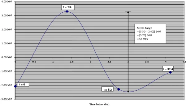
Figure 2: stress range for element 253 at sea state 1
-5.00E+07 -4.00E+07 -3.00E+07 -2.00E+07 -1.00E+07 0.00E+00 1.00E+07 2.00E+07
0 1 2 3 4 5 6 7 8
Time Interval (s)
Fatigue Load
t = 0
t = T/4
t = T/2
t = 3T/4
Stress Range
= [1.30 - (-4.22)] E+07 = [5.52] E+07 = 55.7 MPa
w w w . a j e r . o r g Page 103
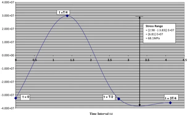
Figure 3: stress range for element 253 at sea state 2
Figure 4: stress range for element 253 at sea state 3
-5.00E+07 -4.00E+07 -3.00E+07 -2.00E+07 -1.00E+07 0.00E+00 1.00E+07 2.00E+07 3.00E+07 4.00E+07
0 1 2 3 4 5 6
Time Interval (s)
Fatigue Load
t = 0
t = T/4
t = T/2
t = 3T/4
Stress Range
= [2.68 - (-4.00)] E+07 = [6.68] E+07 = 66.8 MPa
-3.00E+07 -2.00E+07 -1.00E+07 0.00E+00 1.00E+07 2.00E+07 3.00E+07 4.00E+07
0 0.5 1 1.5 2 2.5 3 3.5 4 4.5
Time Interval (s)
Fatigue Load
t = 0
t = T/4
t = T/2
t = 3T/4
Stress Range
w w w . a j e r . o r g Page 104
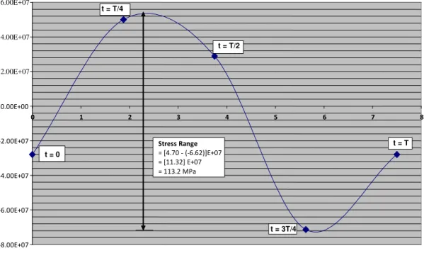
Figure 5: stress range for element 253 at sea state 4
Figure 6: stress range for element 253 at sea state 5
-1.00E+08 -8.00E+07 -6.00E+07 -4.00E+07 -2.00E+07 0.00E+00 2.00E+07 4.00E+07
0 1 2 3 4 5 6 7 8
Time Interval (s)
Fatigue Load
t = 0
t = T/4
t = T/2
t = 3T/4
t = T
Stress Range
= [2.20 - (-8.70)]E+07 = [10.90] E+07 = 109.0 MPa -4.00E+07
-3.00E+07 -2.00E+07 -1.00E+07 0.00E+00 1.00E+07 2.00E+07 3.00E+07 4.00E+07
0 0.5 1 1.5 2 2.5 3 3.5 4 4.5
Time Interval (s)
Fatigue Load
t = 0
t =T/4
t = T/2
t = 3T/4
Stress Range
w w w . a j e r . o r g Page 105
Figure 7: stress range for element 253 at sea state 6
Figure 8: model with applied pressure loads, sea state no.1, t = 0
-8.00E+07 -6.00E+07 -4.00E+07 -2.00E+07 0.00E+00
2.00E+07 4.00E+07 6.00E+07
0 1 2 3 4 5 6 7 8
Time Interval (s)
Fatigue Load
t = 0
t = T/4
t = T/2
t = 3T/4
t = T
Stress Range
w w w . a j e r . o r g Page 106
Table I: Environmental Data
Return periods (yrs)
1 100
Max. wave height in the sea state Hs Hmax m 4.8 7.1
Expected associated or spectral peak wave period Tp sec 15.3 15.7
1 hour average mean wind speed U(1hr) m/sec 12.0 16.3 1 minute average mean wind speed U (1min) m/sec 19.6 32.3 Highest 3 seconds gust in the hour U (3sec) m/sec 21.5 35.5
Surge m 0.25 0.5
Surface current m/sec 1.04 1.44
Current at mid-depth m/sec 0.87 1.21
Current at 1m above sea level m/sec 0.50 0.69
Table II: Most Probable Wave Heights and Time Periods for Different Sea States (Area 59)
Sea State Hs (m) Tp (sec) ζa (m) t (sec) k
1 1 5.5 0.5 4.125 0.133
2 2 5.5 1 4.125 0.133
3 3 6.5 1.5 4.875 0.0961
4 4 7 2 5.25 0.08371
5 5 7.5 2.5 5.625 0.0739
6 6 7.5 3 5.625 0.0739
Table III: Wave Scatter of Area 58, Jan - Dec, ALL DIRECTIONS Sig Hgt
(m) 31 169 311 270 143 54 16 4 1
Obs 1000 > 14 13 to 14
12 to 13 11 to 12 10 to 11
9 to 10 8 to 9 7 to 8
6 to 7
5 to 6 1
4 to 5 1 1 1 1 5
3 to 4 1 6 11 10 6 2 1 36
2 to 3 1 12 46 64 46 21 7 2 198
1 to 2 8 78 176 156 75 24 6 1 524
0 to 1 23 78 83 39 11 2 236
< 4 4 ~ 5 5 ~ 6 6 ~ 7 7 ~ 8 8 ~ 9 9 ~ 10 10 ~ 11
11 ~ 12
12 ~
13 > 13
Zero Crossing Period (s)
w w w . a j e r . o r g Page 107
Table IV: Fatigue Life of joint 33 of Element 253 Sea
State
Stress Range x
SCF (N/mm2)
No. of cycle per year (n)
No. of cycle to failure in Seawater
with Cathodic Protection N(cp)
No. of cycle to failure in Seawater with Free Corrosion
N(FC)
Total number of cycle
to failure,
N
Fatigue Damage
(D)
Estimate d fatigue
life (m)
1 59.60 1354108 1.50E+06 1.12E+06
2.62E+0
6 0.5168 1.93
2 61.00 3006579 1.50E+06 1.20E+06
2.70E+0
6 1.1135 0.90
3 71.50 961293 1.26E+06 1.12E+06
2.38E+0
6 0.4039 2.48
4 72.90 162296 1.21E+06 1.10E+06
2.31E+0
6 0.0703 14.23
5 116.60 21038 1.50E+04 1.30E+04
2.80E+0
4 0.7514 1.33
6 120.90 4208 1.25E+04 1.18E+04
2.43E+0
4 0.1732 5.77
![Figure 1: S-N curves for tubular joints in air, in seawater with cathodic protection, and in seawater with free corrosion [8]](https://thumb-eu.123doks.com/thumbv2/123dok_br/17176458.241598/5.893.151.751.187.455/figure-curves-tubular-seawater-cathodic-protection-seawater-corrosion.webp)