www.atmos-chem-phys.net/10/7369/2010/ doi:10.5194/acp-10-7369-2010
© Author(s) 2010. CC Attribution 3.0 License.
Chemistry
and Physics
Combining visible and infrared radiometry and lidar data to test
simulations in clear and ice cloud conditions
A. Bozzo1,*, T. Maestri1, and R. Rizzi1
1Dipartimento di Fisica, Universit`a di Bologna, Italy
*now at: University of Edinburgh, School of GeoSciences, Edinburgh, UK
Received: 5 December 2009 – Published in Atmos. Chem. Phys. Discuss.: 18 March 2010 Revised: 29 June 2010 – Accepted: 30 July 2010 – Published: 9 August 2010
Abstract. Measurements taken during the 2003 Pacific THORPEX Observing System Test (P-TOST) by the MODIS Airborne Simulator (MAS), the Scanning High-resolution Interferometer Sounder (S-HIS) and the Cloud Physics Li-dar (CPL) are compared to simulations performed with a line-by-line and multiple scattering modeling methodology (LBLMS). Formerly used for infrared hyper-spectral data analysis, LBLMS has been extended to the visible and near infrared with the inclusion of surface bi-directional re-flectance properties. A number of scenes are evaluated: two clear scenes, one with nadir geometry and one cross-track en-compassing sun glint, and three cloudy scenes, all with nadir geometry.
CPL data is used to estimate the particulate optical depth at 532 nm for the clear and cloudy scenes and cloud upper and lower boundaries. Cloud optical depth is retrieved from S-HIS infrared window radiances, and it agrees with CPL values, to within natural variability. MAS data are simu-lated convolving high resolution radiances. The paper dis-cusses the results of the comparisons for the clear and cloudy cases. LBLMS clear simulations agree with MAS data to within 20% in the shortwave (SW) and near infrared (NIR) spectrum and within 2 K in the infrared (IR) range. It is shown that cloudy sky simulations using cloud parameters retrieved from IR radiances systematically underestimate the measured radiance in the SW and NIR by nearly 50%, al-though the IR retrieved optical thickness agree with same measured by CPL.
Correspondence to:R. Rizzi ([email protected])
MODIS radiances measured from Terra are also compared to LBLMS simulations in cloudy conditions, using retrieved cloud optical depth and effective radius from MODIS, to understand the origin for the observed discrepancies. It is shown that the simulations agree, to within natural variabil-ity, with measurements in selected MODIS SW bands.
The impact of the assumed particles size distribution and vertical profile of ice content on results is evaluated. Sen-sitivity is much smaller than differences between measured and simulated radiances in the SW and NIR.
The paper dwells on a possible explanation of these con-tradictory results, involving the phase function of ice parti-cles in the shortwave.
1 Introduction
A recent review of the light scattering properties of cirrus (Baran, 2009) points out that it is more desirable to con-struct cirrus ice crystal models that predict the light scattering properties of non-spherical ice crystals that can be applied at any wavelength rather than at particular wavelengths. It also points out that the choice of ice crystal model, beside its importance for climate modeling, is also important for the space-based remote sensing of cirrus properties, since inap-propriate choice of the scattering phase function may lead to errors in retrieved optical depth of several factors. The re-view contains a wealth of references pertaining to this prob-lem.
Imaging Spectroradiometer, MODIS, retrieved cloud prod-ucts. These are used as input to a radiative transfer model to compute multiply scattered radiances at a number of MODIS channels and comparing the measurements to the simula-tions. The main findings are that radiances for shortwave bands between 0.466 and 0.857 µm appear to be quite accu-rate, while simulated radiances for the 1.24, 1.63 and 3.78 µm bands do not well agree with measurements. Large differ-ences between simulations and data are also found in the in-frared window bands (such those centered at 8.56, 11.0 and 12.0 µm).
In Yang et al. (2007) the differences of the bulk optical properties of ice clouds retrieved in MODIS collection 4 and 5 are investigated and it is shown that collection 5 optical thickness over ocean are a factor 1.9 higher than the collec-tion 4 counterpart. Moreover it is stated that the differences can lead to either an enhancement or a reduction of the warm-ing effect of ice clouds, dependwarm-ing on the specific ice cloud of interest.
In the Zhang et al. (2009) paper, the main concern is the influences of different ice particle micro-physical and opti-cal models on the resulting optiopti-cal thickness retrievals from satellite measurements of solar reflection. They find that the ice cloud optical thickness retrieved from POLDER is sub-stantially smaller than that from MODIS, and the difference is attributed primarily to the difference of asymmetry factor used in the two retrievals. They conclude that ice cloud op-tical thickness retrievals based on satellite measurements of solar reflection are highly sensitive to the choice of the ice particle model assumed in the retrieval.
The present study was initiated to evaluate the quality of a forward modeling methodology, called Line-By-Line Mul-tiple Scattering (LBLMS), that is an extension to the short-wave of a state-of-the-art methodology already used to sim-ulate high resolution spectral data in the infrared spectral range, from 3000 to 50 cm−1(Rizzi et al., 2001; Amorati and
Rizzi, 2002; Maestri and Rizzi, 2003; Tjemkes et al., 2003; Rizzi and Maestri, 2003; Maestri et al., 2005).
Two diverse data sets are used. The first is a field study during the 2003 Pacific THORPEX (The Observing System Research and Predictability Experiment) Observing System Test (P-TOST, http://angler.larc.nasa.gov/thorpex/). During P-TOST the spectro-radiometric data are combined with li-dar products that describe the particulate (aerosol and clouds) extinction profiles. Since our long-term interests are on the retrieval of cloud variables, the experimental cases selected for the core study involve radiances measured in presence of a cloud layer over the marine surface. However the method-ology and results for two clear scenes over the sea are also included, since nadir and cross track simulations of a clear scene provide evidence of correct modeling of the surface and of the aerosol layers, especially in the shortwave (SW) part of the spectrum. This is especially important when deal-ing with thin clouds in order to avoid that incorrect
simula-tions of surface or aerosols properties affect the cloud prop-erties retrieval process.
The second data set is from the Moderate Resolution Imaging Spectroradiometer (MODIS) and corresponding re-trieved cloud products. This data set is used to clarify the un-expected results obtained from the P-TOST cloud cases, and is not intended to present results of statistical significance.
The description of the experiment and of all the case stud-ies is given in Sect. 2, together with the details of the mod-eling methodology. The results for the clear P-TOST case are presented in Sect. 3, the three P-TOST cloudy cases are presented in Sect. 4, and the MODIS computations are dis-cussed in Sect. 5. An overall discussion of the results with conclusions follow in the last section.
2 Description of the experiment and instruments
The P-TOST data-set was measured on 22 and 23 Febru-ary 2003 during a flight over the Pacific Ocean SE of the Hawaiian Islands, when the high altitude NASA aircraft ER-2 carried the three instruments of interest for our analysis: S-HIS, MAS and CPL.
The Scanning High-resolution Interferometer Sounder (S-HIS) (Revercomb et al., 1998) is a Fourier-transform spectrometer with laser-controlled sampling, operating in the thermal spectrum between 3.3 µm and 17.2 µm (3000– 680 cm−1); it utilizes a 45◦scene mirror that rotates through a measurement sequence consisting of views of the earth and two calibration sources, one at ambient and another up to 60 K above ambient. During each scan, 11 cross-track Field of Views (FOVs) are sampled (±35◦total view angle), with
a nadir spatial resolution of 2 km from the nominal 20 km ER-2 flight level and a spectral resolution of 0.5 cm−1.
The MODIS Airborne Simulator (MAS) (King et al., 1996) was built as support to the development of the MODIS satellite instrument: it is a 50 channel scanning spectrometer that covers the spectral range from visible to thermal infrared and acquires 50×50 m (at nadir) pixel data across a 37 km
swath (±43◦view angle) from the nominal ER-2 flight level.
At the nominal ER-2 ground speed of 210 m/s, MAS FOVs show an along-track superposition of the scan lines of about 33% of the pixel width.
The Cloud Physics Lidar (CPL) (McGill et al., 2002) pro-vides cloud and aerosol backscatter profile at 30 m vertical and 200 m horizontal resolution at 1064 nm, 532 nm, 355 nm. During the P-TOST experiment the CPL provided optical depths at 532 nm up to a saturation value of about 3.
In addition to the ER-2, the NOAA G-4 research aircraft flew carrying the Airborne Vertical Atmospheric Profiling System (AVAPS) to measure the temperature and humidity profiles from cruise level (12 km) to the ground.
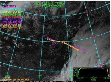
of 20 km and the NOAA G-4 took off 20 min after the ER-2. An overlook of the entire mission’s route can be seen in the GOES image in Fig. 1. At the surface, a high pressure system extends north of the Hawaii islands, smoothly decreasing to-wards the equator. The analysis of the geopotential at higher levels (not shown) reveals an undulation of the tropical jet stream over the eastern Pacific. A ridge extends to the West of Hawaii whereas to the East a trough with an associated slowing down of the jet and upper-level divergence extends towards the equator. The inspection of the vertical velocities at 200 hPa (not shown) shows upwelling on the east side of the trough associated to the extended high cloud cover that can be observed in Fig. 1.
The ER-2 flew from Hickam AFB to get on WNW-ESE oriented track line (20◦N, 153◦W to 16◦N, 144◦W) de-signed to enter and transect subtropical jet zone running up from tropics between 150◦ and 140◦W longitude. ER-2 did 2 back and forth runs (4 total segments) of this line with the G-4 doing profiling on a similar but shorter leg, releasing 11 drop-sondes. G-4 flew back after two ER-2 legs. The Western third of this line contained clear to partly cloudy (low cloudiness) skies. Middle and eastern ends were over-cast with thick cirrus associated with the subtropical flow. Transect crossed core of subtropical jet positioned at about 145◦W.
The P-TOST campaign was designed specifically as a fine tuning opportunity of the MODIS and the Atmospheric In-frared Sounder (AIRS) science product algorithms. The de-cision to use the P-TOST data was taken shortly after the ex-periment was completed, and the choice was based on the following elements: 1) high spatial resolution radiometric data spanning a spectral interval from shortwave to infrared; 2) high spectral resolution infrared interferometric data colo-cated with 1); 3) a clear sky and an ice cloud scenery within the same mission; 4) detailed measurement of the atmo-spheric profile of temperature and humidity and 5) the avail-ability of an airborne LIDAR (on same platform) to provide aerosol products for the clear case and some cloud products for the cloudy one. The campaign would have greatly bene-fited from a satellite overpass, but the closest Terra MODIS granule is at 22:25 of 22 February and covers the upper-eastern part of the GOES image in Fig. 1, outside the experi-mental area. The closest Aqua MODIS granule is at 19:20 of 22 February and covers the eastern edge of the same GOES image, again outside the experimental area.
The P-TOST campaign provides, in the clear case, an in-teresting combination of wind pattern and sun glint to test the surface reflection properties of the modelling suite. Ad-ditional in-situ sampling of the microphysical features of the cloud layer would have been key observations but, to the best recollection of the authors, there were no dataset available at that time with the characteristics described above under 1–5), combined with in-situ microphysical measurements.
Fig. 1. GOES-10 visible channel image, 23 February 2003.
ER-2 route and the drop-sondes positions are shown (from http:// www-angler.larc.nasa.gov/thorpex/).
2.1 Modeling methodology
Although S-HIS and MAS flew together on the ER-2, the data-recording time of the two instruments had different ref-erence, resulting in different time overpass over the same scene. Moreover, it had been noted (R. Holz, University of Wisconsin, Madison, personal communication, 2004) that S-HIS data had wrong geographic data positioning due to use of the inertial navigation system of the ER-2 as reference, which in the analyzed mission did not work properly. There-fore a scheme was developed to collocate MAS and S-HIS data using MAS channel 45 (a window centered at 11 µm). This channel performs a relatively more stable measurement of the scene radiance with respect to window channels lo-cated in NIR range, which are affected, moreover, by solar contribution. Two sets of virtual measurements are gener-ated, having the spatial resolution of S-HIS and the spec-tral resolution of MAS: MAS pixels are averaged over the S-HIS footprint closest to nadir and the S-HIS data is con-volved over the MAS spectral response function to produce the equivalent MAS spectral bands (Moeller et al., 2003). The minimisation of the mean square differences between the convolved S-HIS signal and the averaged MAS signal is performed over a 750 km long ER-2 track (corresponding to flight between 01:06 UTC and 02:00 UTC on 22 February) in which clear sky, broken clouds and overcast situations are present. The mean temporal displacement between MAS and S-HIS data is found to be 41±2 s. The uncertainty of 2 s pro-duces a possible spatial displacement of about 400 m at the nominal ground speed of the ER-2, i.e. it is smaller than the linear dimension of the S-HIS nadir footprint.
scattering properties (that change from layer to layer). The simulations are done with a suite of codes collectively called Line-By-Line Multiple Scattering (LBLMS). In the present work the line-by-line computations of layer spectral optical depths are done using the Line-by-Line Radiative Transfer Model (LbLRTM) (Clough and Iacono, 1995). LbLRTM can solve the clear sky radiative transfer equation, but in our study is used to generate layer monochromatic optical depths (OD). These are interpolated at 0.002 cm−1 and then con-volved to compute spectrally averaged OD.
Tests were done to find the appropriate spectral resolu-tion for the specific sensors that are modeled (S-HIS and MAS in this work), so that the difference between radi-ances convolved using the averaged optical depths or directly the LbLRTM monochromatic radiances were below a given threshold. Results are dependent on the spectral widths over which the OD average is performed and also on the atmo-spheric layering. Three different spectral resolutions were used, as a compromise between a reasonable computing time and accuracy: 0.01 cm−1 from 580 to 3000 cm−1 (3.33– 17.2 µm, indicated as IR in this paper), 0.05 cm−1from 3000 to 7000 cm−1(NIR, 1.43–3.33 µm), and 0.5 cm−1from 7000 to 22 000 cm−1 (SW, 0.45–1.43 µm). The HITRAN 2004 (Rothman et al., 2005) spectroscopic database and the MT-CKD 1.3 water vapour continuum absorption model (Clough et al., 2005) are used.
The integration of the radiative transfer equation, includ-ing multiple scatterinclud-ing, is based on the code RT3 (Evans and Stephens, 1991). Layer spectral absorption optical depth is the sum of molecular and particle absorption and spectral to-tal scattering optical depth is the sum of particle and Rayleigh scattering with the total phase function being a weighted mean of the two components.
The emissivity of the ocean surface in the IR is computed using the method described in Masuda et al. (1988). The ocean surface reflection properties take into account the con-tribution from the wind-roughened surface (Cox and Munk, 1954), the white caps and the up welling radiation scattered back from below the surface as function of the oceanic pig-ment concentration. The surface model implepig-mented in RT3 is analogous to the one adopted in 6S (Vermote et al., 2006), with the only exception being the wind direction dependency that in RT3, due to limitations inherent to its computational structure, is not allowed. An in depth description of the meth-ods adopted can be found in Bozzo (2009).
Post-processing of high resolution radiances to produce un-apodised spectra at S-HIS resolution is done as described in Rizzi et al. (2001). Simulated MAS radiances are obtained by convolving the spectral values at the indicated resolution with the MAS response functions (NASA, cited 2008).
Aerosol single scattering optical depth and phase function are computed using an in-house code, but the main physics contained (refractive index of components, aerosol as a col-lection of homogeneous spherical particles, size distribu-tions, definition of external mixtures and growth coefficients)
is analogous to the package OPAC (Hess et al., 1998) and so are the computed properties. The Mie scattering portion is handled by routines distributed together with the initial ver-sion of the RT3 code by Frank Evans.
The retrieval methodology (RT-RET) is described (and applied to Arctic and Mid latitude clouds respectively) in Maestri and Holz (2009) and Maestri et al. (2010). RT-RET uses LbLRTM and the same doubling and adding algorithm (RT3) described earlier. In this paper it is used to retrieve cloud optical depths and effective dimension of the cloud particle size distribution (PSD) from S-HIS radiances. The definition of effective dimensionDeof a PSD made of
non-spherical shaped particles is the same that was introduced by Foot (1988):
De=
3 2
Z Dmax
Dmin
V (D)n(D)dD
Z Dmax
Dmin
P (D)n(D)dD
(1)
whereP (D) andV (D)are respectively the projected area and volume of a particle with maximum dimensionD. The ice densityρi is assumed constant with the particle
dimen-sion. Effective radius is defined asRe=De/2.
The single scattering properties for different ice habits in the short-wave (0.25–4.5 µm) and long-wave (4.5–100 µm) spectral ranges are taken from Yang and Liou (1998) and Yang et al. (2005) and will be referred to in the following by the acronyms SSP-SW and SSP-IR.
Previous work (e.g. Wendisch et al., 2005; Wyser, 1999) has shown large differences in simulations based on PSD composed of single shapes and there are no reasons to pre-fer one shape over another. Our choice is to use a mixture (called MIXML) of different habits, bullet rosettes, aggre-gates, droxtals and a small percentage of solid columns as described in Bozzo et al. (2008) and Fig. 1 of the quoted paper. MIXML is based on Lawson et al. (2006) measure-ments, developed in the context of mid latitude ice clouds. The major differences between mid-latitude and tropical cir-rus clouds are found for cirri formed near strong tropical con-vective events, at the top of large anvils. Such ice clouds present usually higher fractions of larger particles than mid latitude-synoptic ice clouds, associated to strong updrafts (Baum et al., 2005). In case of synoptically generated mid-latitude cirrus, the large ice crystals tend to subside quickly due to the weak updrafts. In our case, although the cirrus is associated with the subtropical jet-stream, it does not show the characteristics related to the tropical convective struc-tures. MIXML has been tested in the analysis of infrared interferometric data collected at Mid Latitudes and in cloudy conditions during the italian phase of the EAQUATE experi-ment (Maestri et al., 2010).
The ice particle size distribution (PSD) adopted for the for-ward and inverse computations is a Gamma distribution:
0 20 40 60 80 100 120 140 160 180 10−1
100 101 102
PF
0 20 40 60 80 100 120 140 160 180
−0.4 −0.2 0 0.2 0.4
Scattering Angle, degree
(PF−PFR)/PF
O − 0.45 µ m R − 0.45 µ m O − 0.82 µ m R − 0.82 µ m
0.45 µ m 0.82 µ m
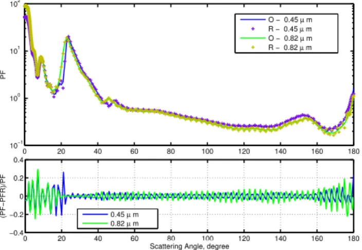
Fig. 2.Upper panel: phase functions in the shortwave at 0.45 µm:
Original (PF, blue line) and Reconstructed (PFR, purple crosses); PF at 0.82 µm: Original (green line) and Reconstructed (olive green crosses). Lower panel: fractional difference computed as (PF-PFR)/PF.
whereD is the particle maximum dimension,N0is the
in-tercept value of the distribution,λthe slope (with unit of an inverse dimension) andµis the dispersion (or shape) param-eter. The PSD is extended to particles smaller than the one available in the quoted databases by assuming that spher-ical particles are present with diameter smaller than 2 µm, whose properties are computed using same Mie code as for the aerosol properties.
Particular attention has been given to the treatment of the phase function to account for the sharp diffraction peak exhibited by the ice crystals. Since the scattering phase function is handled with an expansion in Legendre poly-nomials, such peaked functions would require thousands of components, which in turn would imply an extremely time-consuming solution. Instead, the procedure proposed by Pot-ter (1970) has been followed and the phase function peak is modified by using a spectrally varying algorithm which is tailored to minimise the number of Legendre terms required for an accurate reconstruction. The contribution of the delta-transmission peak associated with the forward scattering at a 0◦(Takano and Liou, 1988) is also accounted for. The num-ber of Legendre terms used in the computation is linked to the number of angles employed in the zenith discretization in each hemisphere (Nu). After considerable tests we have
used, for the ice cloud cases, Nu=32 (and 125 Legendre
terms) in all spectral regions except from 600 to 4850 cm−1 whereNuis set to 60 (237 Legendre terms). Since the CPU
time required for LBLMS computation is proportional to the cube ofNu, the accurate computation of high resolution
ra-diances has required a massive computational effort that was made possible only after code parallelisation.
Fig. 3. MAS imagery on Pacific Ocean SE from Hawaiian Islands
on 22 February 2003, from 23:01 to 23:05 UTC (roughly 50 km on the ground). The RGB image is obtained from channels 20 (2.15 µm), 10 (1.64 µm), 2 (0.55 µm). The blue line and the red box show the regions chosen for the cross-scan and nadir comparisons.
As an example in Fig. 2 the original phase function, after truncation using Potter’s method, is shown together with the one reconstructed with a number of Legendre coefficient as explained above. The figure shows that the fractional differ-ence is an oscillating function that is generally below 10% except at some specific angles where it can reach values be-tween 20% and 30%. The geometry of the nadir measure-ment in the cloudy case is such that the (single) scattering angle is 123◦.
3 Description of the clear cases and results
3.1 Measurement conditions for the clear cases
0.5 0.55 0.6 0.65 0.7 0.75 0.8 0.85 0.9 0.95 0
20 40 60
Wavelength µm
Radiance W/
µ
m m
2 sr
1.6 1.7 1.8 1.9 2 2.1 2.2 2.3 2.4
0 1 2
Wavelength µm
Radiance W/
µ
m m
2 sr
800 1000 1200 1400 1600 1800 2000 2200 2400 2600 2800
220 240 260 280 300
Wavenumber cm−1
B.T. (K)
MAS LBLMS
Fig. 4.Comparison of LBLMS simulations and MAS observations
at nadir in clear sky conditions. Top and mid panel: comparison of upwelling radiance at 20 km; lower panel: IR brightness tempera-ture.
pixel long area, which covers a section 2◦wide (±1◦across the nadir line) and roughly 15 km long, along the blue line in Fig. 3. For the cross-track case MAS measurements are av-eraged over an area as wide as the full MAS swath and 120 pixel long (the red box on Fig. 3), which roughly corresponds to a 4 km long and 40 km wide region.
In both case studies the averaged MAS data is compared to the LBLMS simulation. The solar zenith angle is approx-imately 31◦ and solar azimuth 204◦; sensor azimuth angle swings between 204 and 24◦, hence aligned with the surface incidence plane of solar radiation.
Three drop-sondes were launched in coincidence with this track: one at 23:07 UTC, the second at 23:12 UTC and the third at 23:17 UTC. All drop-sondes measured a 10 m wind speed between 6 m/s and 7 m/s with azimuthal direc-tion around 30◦, hence slightly skewed with respect to the instrument-sun plane: wind speed has been set in the sim-ulation at 6.5 m/s. The vertical profile of temperature and humidity used for the simulation is a composite of the data from the 23:17 UTC drop-sonde and a standard tropical pro-file (Anderson et al., 1986) to fill the 10 km gap between the G-4 and the ER-2 cruise altitude. The CO2mixing ratio
pro-file is modified to measured global mean value for the pe-riod of the campaign. Absorption from chloro-fluoro-carbon macro molecules (CFC) is also accounted for.
The CPL detected the presence of an aerosol layer dis-tributed in the boundary layer from 1000 m down to about 500 m. Below this level there is no information on aerosol optical depth. Since the source of aerosol is the oceanic surface an exponential extrapolation of the measured optical depth profile down to the marine surface is assumed. The integrated optical depth at 532 nm obtained with this
pro-0.5 0.55 0.6 0.65 0.7 0.75 0.8 0.85 0.9 0.95
−0.4 −0.2 0
Wavelength (µm)
(LBLMS−MAS)/MAS
1.6 1.7 1.8 1.9 2 2.1 2.2 2.3 2.4
−1 −0.5 0 0.5
Wavelength (µm)
(LBLMS−MAS)/MAS
800 1000 1200 1400 1600 1800 2000 2200 2400 2600 2800
0 2 4 6
LBLMS−MAS (K)
Wavenumber cm−1
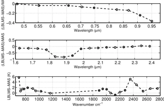
Fig. 5. Differences between LBLMS simulations and MAS
obser-vation at nadir in clear sky conditions. Top and mid panel: rela-tive radiance errors (LBLMS-MAS)/MAS; lower panel: absolute IR brightness temperature difference (LBLMS-MAS, K).
cedure is 0.07. Because of the extremely low aerosol load measured by CPL, such an extrapolation must be considered only a minor weakness in the definition of our study case. As already mentioned there is no MODIS data over the experi-mental area and no aerosol product different from the CPL one is thus available. The aerosol layers (from surface to 1000 m height) are simulated with the optical characteristics of a maritime tropical aerosol model (same mixture defined in Hess et al. (1998), grown in an ambient with 80% rela-tive humidity, in accordance with the drop-sondes measure-ments).
The pigment concentration of the oceanic water derived from the global products of the SeaWiFS satellite (Johnson et al., 1998), averaged over 8-days around the 22 Febru-ary 2003 in the Pacific Ocean SE of the Hawaiian Islands, has a mean value of 0.07 mg/m3.
3.2 Results for the clear nadir case
signal provided by the clear sky scene. The channel centered at 1848 cm−1did not work properly during the selected
mis-sion and has been ignored in the comparison.
The difference between the simulations and the MAS data is almost constant in the SW range between 0.45 and 1 µm with a value of about 1.5 W/(m2µm sr), hence the relative er-ror increases with increasing wavelength since the radiance level is decreasing: it remains below 10% for wavelength shorter than 0.7 µm and it grows up to 35% approaching the channels at 0.95 µm. In the NIR range the relative error is around 10–15% with the exception of the strong H2O band,
where it reaches values of about 90%.
In the IR, from 500 cm−1to 2800 cm−1, the absolute er-rors are between 0.5 and 2 K except in the 3 channels located in the strong CO2absorption bands (one at 700 cm−1and the
other two at 2250 and 2450 cm−1). The discrepancy in the
opaque channels due to CO2absorption is certainly linked to
the assumed atmospheric temperature profile . The surface skin temperature is set equal to the last temperature measured by the drop-sonde and this affects the simulation in the win-dow regions. These differences could be easily eliminated to a large extent by improving the assumed atmospheric/surface temperature profile but in this case study we were not par-ticularly concerned with the small deviations in the infrared range and we did not optimise those computations.
The largest relative differences in the SW and NIR are found in channels with important water vapour absorption. We have performed simulations also of the S-HIS data (not shown) and the results show a negative bias (the simula-tion being colder that the S-HIS data) in the infrared vibro-rotational band of water vapour. Therefore the water vapour profile, and in particular the profile assumed between the G-4 and the ER-2 flight levels, is likely more humid than the true profile, which also explains the negative bias in the SW and NIR channels.
In conclusion the main causes of the observed discrepan-cies in the SW and NIR could be the modeling of the scatter-ing by the oceanic surface, the assumed aerosol optical depth vertical profile, the aerosol mixture adopted and its growth properties. Each of these will be discusses in what follows.
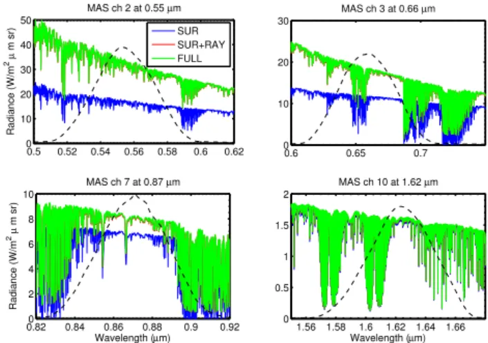
To understand the importance of each process, the four panels of Fig. 6 show the upwelling radiance at MAS height simulated for four channels when a) the source function is the surface with a molecular atmosphere that only absorbs radiance (line labeled SUR in all panels), b) when molecular scattering is added as source of radiance (SUR+RAY) and finally c) when aerosol is also present (FULL). It is evident that in our case study the surface and molecular scattering are the dominant radiation sources.
Currently our modeling of the oceanic surface assumes that the sun glint pattern is independent on the wind direc-tion. Comparisons with the 6S model indicate that this hy-pothesis gives an error in the range 10–20% of the signal for low solar zenith angles (Bozzo, 2009). In particular, in case of a zenith angle of 31◦the up-welling radiation is enhanced
0.5 0.52 0.54 0.56 0.58 0.6 0.62 0
10 20 30 40 50
Radiance (W/m
2µ
m sr)
MAS ch 2 at 0.55 µm
0.6 0.65 0.7 0
10 20 30
MAS ch 3 at 0.66 µm
0.820 0.84 0.86 0.88 0.9 0.92 2
4 6 8 10
Wavelength (µm)
Radiance (W/m
2µ
m sr)
MAS ch 7 at 0.87 µm
1.56 1.58 1.6 1.62 1.64 1.66 0
0.5 1 1.5 2
Wavelength (µm) MAS ch 10 at 1.62 µm SUR
SUR+RAY FULL
Fig. 6. High resolution spectral radiance in four MAS channels:
channel 2 (top left), channel 3 (top right), channel 7 (bottom left) and channel 10 (bottom right). The colour coding is same for all the panels: the blue line labeled SUR is the case when the surface is the sole source function with a molecular atmosphere that only ab-sorbs radiance; the red curve labeled (SUR+RAY) is radiance after molecular scattering is added; the green line (FULL) considers also the presence of aerosol as source function and absorber. The dashed black line is MAS Relative Response Function on a relative scale.
if the wind is blowing along the incident and reflected solar beam plane, whereas it is reduced in case of a wind blow-ing orthogonal to the sun’s reflection plane. The wind’s az-imuthal angle retrieved from the drop-sondes measurements is around 60◦, hence 36◦ from the sun’s reflection plane, which lies along the 24◦–204◦azimuthal line.
The OPAC standard Maritime tropical aerosol model is an external mixture of three components, one of which, the sea salt coarse mode (SSCM) accounts for 1.4% of the mass of the mixture. The extinction optical depth has a maxi-mum around 5 µm decreasing toward shorter wavelengths, markedly different from the sea salt accumulation mode component (SSAM) which has a maximum around 1 micron. Therefore one could devise a slightly different mixture, by increasing the mass of the SSCM and reducing the mass of SSAM, and the new mixture would reduce the underes-timation observed in the NIR. Also data on condensational growth by aerosol components is sparse, and it is well known that assuming aerosols are spherically homogeneous parti-cles is only a rough approximation. However the relevance of the aerosol contribution is so small in this case study that it is not necessary to dwell on the various sensitivity tests performed.
−40 −30 −20 −10 0 10 20 30 40 0
0.02 0.04 0.06 0.08 0.1 0.12 0.14 0.16 0.18 0.2
view angle (deg from nadir)
Reflectance
0.55 µm
0.66 µm
0.87 µm
1.62 µm
Fig. 7.Reflectance comparison between LBLMS (dashed lines) and
MAS (continuous lines) along a MAS scan. Wind speed is 6.5 m/s, aerosol OD at 532 nm 0.07 and pigment concentration 0.07 mg/m3.
In the next section we examine the same scenario, but from different viewing angles.
3.3 Results for the clear cross-track case
LBLMS is tested with a full MAS cross-track scan swinging in the analyzed scene from the maximum to the minimum of the glint reflection region, along the reflection plane of the incoming solar radiation. Up-welling radiation at 20 km is simulated at 32 zenith angles for each hemisphere using 64 terms of the azimuthal-mode Fourier expansion. Pigment concentration, aerosol profile, model and relative humidity are same for the nadir case. Figure 7 shows the reflectance at 20 km for 4 MAS channels defined in the previous section. The BDRF for various wavelengths is computed from aver-aged MAS data (full lines) inside the red box in Fig. 3, and from LBLMS simulations (dashed lines).
The peak in reflectance is reached for all the 4 curves at around 36◦, slightly shifted toward the horizon from the Fres-nel reflection point that is supposed to be at the incidence angle of 31◦. The glint pattern appears to be less steep and slightly more skewed towards the horizon in the MAS ob-servations: in fact some difference in the glint pattern is ex-pected due to the assumption of a wind direction-independent BDRF in the simulations.
The relative difference are between−10% to+10% over
the whole scan for the SW channels, with a larger underesti-mation for the NIR channels, and are largest in the direction opposite to the reflection point, at minimum MAS radiance values.
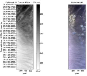
Fig. 8.Cloudy sky scenario. MAS imagery from track 9, 23
Febru-ary 2003 on Pacific Ocean SE from Hawaiian Islands from 01:26 to 01:33 UTC. Infrared brightness temperature from channel 45 is presented on left panel. RGB image (right panel) is obtained from channels 20 (2.15 µm), 10 (1.64 µm), 2 (0.55 µm).
4 Description of the cloudy cases and results
4.1 Measurement conditions for the three cloudy cases
As already mentioned the ER-2 did 4 segments and the mid-dle and eastern end of the flight leg were characterized by an extended cirrus associated with the subtropical jet-stream. The transect crossed the jet at about 145◦W and 19–20◦N. The ER-2 made two back and forth overpasses over the high, thick tropical cirrus.
As pointed out in the discussion of the clear cases, some assumptions adopted in the ocean’s reflectivity model imple-mented in LBLMS could lead to spurious effects in the in-terpretation of the upwelling radiance, especially at low sun zenith angles. For this reason all measurements between the ER-2 take off time and 24:00 UTC (14:00 local time) were disregarded. The chosen transect is located between 01:26– 01:34 UTC and is characterized by a solar zenith angle of 57◦.
Thermal infrared and visible MAS imagery show (see Fig. 8) that the cloud is fairly homogeneous only in the opti-cally thickest part and quite variable elsewhere. The thinnest part, located at the edge of the very extended cloud layer, is rather inhomogeneous with many open gaps over the un-derlying ocean. Some small cumulus clouds can be spotted below the cirrus layer, although not directly beneath the flight line.
Altitude [km]
Time (UTC) hh:mm:ss
01:07:180 01:16:27 01:25:18 01:34:09 01:43:27 01:52:49 5
10 15 20
0.5 1 1.5 2 2.5 x 10⁻³
Fig. 9. CPL extinction cross section from 01:07 to 01:54 UTC on
the 23 February 2003. Pixels with integrated optical depth smaller than 0.02 are coloured white. Black pixels are those with integrated optical depth greater than 2.98, that is where the signal is saturated, or to pixels for which no CPL measurement is available.
chosen ER-2 sector, but from satellite imagery there seem to be no important cloud development in these two hours. In the humidity profile, the cloud layer position is character-ized by a net increase of relative humidity between 200 hPa and 300 hPa up to a value of 60% in the middle of the layer for the section with the optically thickest cloud. As in the clear sky case, a sub-tropical climatological standard profile is used to fill the gap between the two aircrafts. As an esti-mate of the surface wind speed we use the same wind speed adopted in the clear sky scene (6.5 m/s), though the relative importance of the surface wind in absence of a sun glint is very small. The pigment concentration and the aerosol op-tical depth, profile and mixture are the same adopted in the clear sky case.
For layers with optical depth at 532 nm less than 3, CPL data is used to characterize the internal cloud structure and to define top and bottom cloud levels. Figure 9 shows the ex-tinction cross section at 532 nm at nadir for the flight stretch chosen for the comparison. The cloud becomes thicker and the top height increases while flying from the edge of the cloud layer to the inner part.
The CPL optical depth at 532 nm is shown in Fig. 10 and it is seen that after 01:34 UTC the CPL signal is saturated, hence the cloud bottom information is not reliable. Three sectors are selected from the whole track: they are repre-sentative of a very thin (between red lines in Figure 10), a medium thin (green lines) and a moderately thick (blue lines) cirrus layer.
1.26 1.27 1.28 1.29 1.3 1.31 1.32 1.33 1.34
x 104
0 0.5 1 1.5 2 2.5 3 3.5 4 4.5 5
time UTC (hmm)
OT
CPL OT (532nm)
Fig. 10.CPL retrieved cloud total optical depth for the ER-2 flight
leg from 01:26 to 01:34 UTC, 23 February 2003. The vertical coloured lines delimitate the three sectors selected for the compar-isons.
The retrieval methodology RT-RET is used to determine cloud optical thickness (OT) and effective dimension De
from S-HIS data, collocated with MAS data, averaged over each of the three sectors selected. A-priori parameters (to be defined before the actual retrieval can be done) are: the µ parameter of the size distribution, the ice crystal shape and the bottom and top heights of the cloud layer. The re-trieval, moreover, assumes that the IWC is distributed homo-geneously with height.
In next section the retrievals and the forward computations for a standard case (called V0) defined with a specific choice of these parameters, are shown. Since no measured data is available from the field campaign about the micro-physical composition of the cirrus layer, we have used MIXML, for reasons already discussed. The size distribution is described by a Gamma with a value ofµ=0. Cloud top and cloud
bot-tom are the average in each sector of the values determined from CPL measurements collocated with S-HIS FOVs. Other choices are possible: in regions where the CPL signal is not saturated, the extinction profile can be used to infer the IWC vertical distribution (assuming a vertically invariant constant composition and size distribution). A comparisons of results obtained with an IWC that varies with height versus the ho-mogeneous case is shown in Sect. 4.3. In Sect. 4.4 results are presented that assume different values of theµparameter of the PSD (cases V1 and V2).
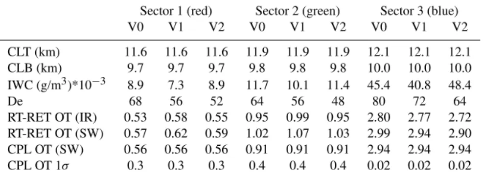
Table 1.Characteristics of the 3 cloudy sectors used for the comparisons. CLT and CLB are cloud top and bottom height obtained rom CPL; RT-RET OT (IR) andDe, hence IWC, are retrieved by RT-RET averaged in each sector; CPL OT is measured by CPL at 532 nm and CPL
OT 1σ is one standard deviation of measured CPL OT in each sector.
Sector 1 (red) Sector 2 (green) Sector 3 (blue) V0 V1 V2 V0 V1 V2 V0 V1 V2 CLT (km) 11.6 11.6 11.6 11.9 11.9 11.9 12.1 12.1 12.1 CLB (km) 9.7 9.7 9.7 9.8 9.8 9.8 10.0 10.0 10.0 IWC (g/m3)*10−3 8.9 7.3 8.9 11.7 10.1 11.4 45.4 40.8 48.4 De 68 56 52 64 56 48 80 72 64 RT-RET OT (IR) 0.53 0.58 0.55 0.95 0.99 0.95 2.80 2.77 2.72 RT-RET OT (SW) 0.57 0.62 0.59 1.02 1.07 1.03 2.99 2.94 2.90 CPL OT (SW) 0.56 0.56 0.56 0.91 0.91 0.91 2.94 2.94 2.94 CPL OT 1σ 0.3 0.3 0.3 0.4 0.4 0.4 0.02 0.02 0.02
determine the total ice mass for the whole depth of the cloud (IWP) and then used to compute the OT at 532 nm using the same PSD, type of mixture and optical properties database: such OT values agree within the natural variability of the OT values derived from CPL, also shown in Table 1 in the three sectors.
Figure 11 shows the brightness temperature in MAS chan-nels obtained by averaging MAS pixels over the S-HIS foot-prints in each sector, and the corresponding S-HIS data (av-eraged in each sector) convolved over the MAS spectral re-sponse function. The agreement between the instruments is quite good throughout most of the IR spectrum.
4.2 Results for the standard cloudy cases
LBLMS is used to simulate the upwelling radiance from the three sectors highlighted in Fig. 10 over the whole spectral range covered by MAS, using the same configuration as in the clear sky case.
Figures 12, 13 and 14 show the comparison between MAS measurements and LBLMS simulations in the three cloud sectors. Figure 15 shows the relative difference between LBLMS simulations and MAS measurements.
Since the procedure RT-RET is based on an iterative least square fit of the S-HIS radiance between 820 and 980 cm−1 the agreement between the observations and the simulations in that range is obviously quite good. Agreement between data and simulations (accounting for one standard devia-tion of the MAS data) is in fact found between 1200 and 650 cm−1, in all the sectors. The difference between LBLMS
and MAS lies between−2 K and+2 K, with an overestima-tion for the thin cloud and a slight underestimaoverestima-tion for the other two cases, but well inside the signal variability over the scene, represented by one standard deviation of the MAS data around the mean value. All the simulations show a narrow overestimation region at about 1050 cm−1due to in-complete information about the O3atmospheric profile. For
wavenumber greater than 1800 cm−1 the signal is the sum of the radiation emitted at terrestrial temperatures and of the
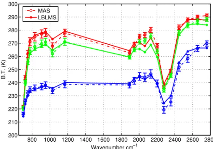
800 1000 1200 1400 1600 1800 2000 2200 2400 2600 2800 200
210 220 230 240 250 260 270 280 290 300
Wave−number (cm−1)
Brightness Temperature (K)
MAS SHIS
Fig. 11.MAS data averaged over S-HIS nadir FOV and S-HIS data
convolved with MAS relative spectral response. The red solid line and yellow dashed refer to Sector 1 (the thin cloud layer); the two green shades are for Sector 2 (medium cloud layer) and the blue lines are for the moderately thick layer of Sector 3. The vertical bars are the one standard deviation of the MAS data around the average values and denote the natural variability as well as radiometric error.
reflected solar radiation and the influence of the latter is evi-dent in the spectral ranges where the brightness temperature is higher than that observed in the IR window. LBLMS un-derestimates MAS in the red and green sectors between 2000 and 2200 cm−1, while overestimates in the blue sector be-tween 2300 and 2700 cm−1.
0.5 0.55 0.6 0.65 0.7 0.75 0.8 0.85 0.9 0.95 0
20 40 60 80 100 120 140 160 180
Wavelength (µm)
Radiance (W/
µ
m m
2 sr)
MAS LBLMS
Fig. 12.LBLMS simulations and MAS observations in cloudy
con-ditions – SW range. The three colours represent the three sections highlighted in Fig. 10: red for the thin cloud layer, green for the medium cloud layer and blue for the moderately thick layer. The vertical bars have same meaning as in Fig. 11.
1.6 1.7 1.8 1.9 2 2.1 2.2 2.3 2.4
0 5 10 15
Wavelength (µm)
Radiance (W/
µ
m m
2 sr)
MAS LBLMS
Fig. 13.Same as Fig. 12 but for the NIR spectral range.
4.3 Homogeneous versus inhomogeneous cases
The results for the standard (homogeneous) case are consis-tent with RT-RET that retrieves cloud parameters assuming that the cloud is vertically homogeneous. In this section the CPL derived cloud extinction profile is used to modulate the amount of ice mass within the cloud layer, in each sector. We have used the same De constant with height, as in the
standard case.
The cloud properties are then used to calculate the total ice amount so that the OT, computed at 532 nm, matches the CPL one (given in Table 1). The average CPL extinction profiles for the three chosen sectors are shown in Fig. 16. The extinction profiles are interpolated at the model levels (computations in sectors 1/2/3 are done with 11/14/14 cloud layers, of thickness 0.2 km, out of 81 layers to describe the atmosphere) and the IWC profile is computed so that it is
800 1000 1200 1400 1600 1800 2000 2200 2400 2600 2800
200 210 220 230 240 250 260 270 280 290 300
Wavenumber cm−1
B.T. (K)
MAS LBLMS
Fig. 14. IR brightness temperature from LBLMS simulated and
MAS observed radiance at 20 km. The three colours represent the three sections highlighted in Fig. 10. The vertical bars have same meaning as in Fig. 11.
0.5 0.55 0.6 0.65 0.7 0.75 0.8 0.85 0.9 0.95
−0.5 0
Wavelength (µm)
(LBLMS−MAS)/MAS
1.6 1.7 1.8 1.9 2 2.1 2.2 2.3 2.4
−1 −0.5 0
Wavelength (µm)
(LBLMS−MAS)/MAS
800 1000 1200 1400 1600 1800 2000 2200 2400 2600 2800
−10 0 10
LBLMS−MAS (K)
Wavenumber (cm−1)
Fig. 15.Differences between LBLMS simulations and MAS
obser-vation in cloudy conditions. Top and mid panel: relative radiance errors (LBLMS-MAS)/MAS; lower panel: absolute IR brightness temperature difference (LBLMS-MAS, K). The three colours rep-resent the three sections highlighted in Fig. 10.
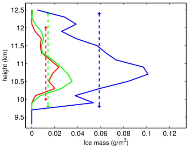
proportional to the average extinction profile. The final IWC profiles are shown in Fig. 17.
0 0.5 1 1.5 10
10.5 11 11.5 12 12.5
Ext. Coeff. (km−1)
Height (km)
Fig. 16.Average extinction profile for Sector 1 (red), 2 (green) and
3 (blue) derived from CPL.
0 0.02 0.04 0.06 0.08 0.1 0.12
9.5 10 10.5 11 11.5 12 12.5
Ice mass (g/m3)
height (km)
Fig. 17.Average IWC profile, for the LBLMS layering, for Sector
1 (red), 2 (green) and 3 (blue) derived as explained in the text. The vertical dashed lines indicate the profiles adopted for the homoge-neous computations.
1.8 and 1.9 µm, where molecular absorption is relevant. For the case under study, the inhomogeneity reduces the scattered radiance to the sensor with respect to the standard case.
These results show quite clearly that the difference in sim-ulated radiance between the homogeneous and the inhomo-geneous cases are, in any case, much smaller than the differ-ence between measured and simulated radiances described in Sect. 4.2.
4.4 Results with different PSDs
Small particles are strong scatterers of solar radiation, though they bring small contribution to the total PSD’s mass and one could imagine that one of the causes of the radiance under-estimation is due to an improper treatment of the PSD in the small particle range.
0.5 0.55 0.6 0.65 0.7 0.75 0.8 0.85 0.9 0.95
−0.1 −0.08 −0.06 −0.04 −0.02 0
Wavelength (µm)
(inhom−hom)/hom
1.6 1.7 1.8 1.9 2 2.1 2.2 2.3 2.4
−0.1 −0.05 0 0.05 0.1
Wavelength (µm)
(inhom−hom)/hom
s1 s2 s3
Fig. 18. Fractional difference (Inhom-Hom)/Hom between the
in-homogeneous and the in-homogeneous cases for the three sectors, in the shortwave (top panel) and near infrared (bottom panel) MAS channels.
There is in fact much discussion on the role of small ice particles (whose effective diameter is smaller than about 50 to 60 µm) and on the physical mechanisms that produce and eventually maintain these particles inside cirrus clouds. Jensen et al. (2009) report on new aircraft measurements in anvil cirrus sampled during the Tropical Composition, Cloud, and Climate Coupling (TC4) campaign with the 2-Dimensional Stereo (2D-S) probe, which can detect particles as small as 10 µm. They suggest that micro-physical mea-surements in tropical cirrus clouds obtained with the CAS (Cloud Aerosol Spectrometer) should be considered suspect when large crystals are present, and that measurement made with instruments at the wing-hatch location are presumably also affected by shattering artifacts. They however point out that their findings are relevant for relatively low and warm tropical cirrus and do not imply that small crystals do not play a significant role in the radiative properties of other types of cirrus, such as anvils generated by continental con-vection, mid-latitude cirrus, or even anvil cirrus in other trop-ical regions. They also point out that small particles could persist in uppermost tropical tropopause which is often satu-rated with respect to ice.
The sensitivity of the results to the assumed set of PSDs is here investigated. The main parameter defining each set of PSDs is the dispersionµ. For each value ofµ(i.e. each PSD set) the slopeλis varied so that 26 PSDs are defined by their effective dimensionDe. Typical values of the dispersion
range between−2 and 16, while typical slopes range from 0.1 to 10−4cm−1(withDexpressed in cm). These values are derived from data discussed in Baum et al. (2005) and Heymsfield et al. (2004), where measured PSDs of ice clouds from six field experiments are fitted to theoretical modified gamma type PSDs. The intercept N0 determines the total
0.5 0.55 0.6 0.65 0.7 0.75 0.8 0.85 0.9 0.95 −0.05
0 0.05
Wavelength (µm)
(Vx−V0)/V0
1.6 1.7 1.8 1.9 2 2.1 2.2 2.3 2.4
−0.1 0 0.1
Wavelength (µm)
(Vx−V0)/V0
800 1000 1200 1400 1600 1800 2000 2200 2400 2600 2800 −0.5
0 0.5
K
Wavenumber cm−1
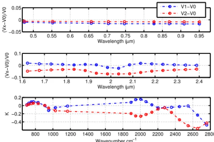
V1−V0 V2−V0
Fig. 19.Comparison between radiance simulated for cases V0, V1,
V2 for Sector 1. Top and middle panels: fractional radiance dif-ference with respect to V0; lower panel: brightness temperature difference with respect to V0.
Two new sets of size distributions (each consisting of 26 PSDs for each set) were defined with the values µ=7.0
(called V1) andµ= −0.1 (called V2), and for each set
RT-RET is used to retrieve the corresponding OT andDe.
Ta-ble 1 contains the retrieved cloud parameters for the three sectors and the two PSD sets (V1 and V2), besides the re-sults for the standard case (V0).
The three retrieved PSDs are used to simulate the spectral radiance at high resolution in each of the three sectors, and the S-HIS and MAS convolved radiances. The difference among the results for cases V1 and V2 are plotted in Fig. 19, Fig. 20 and Fig. 21 respectively for Sectors 1 to 3. Fractional radiance difference(L(V x)−L(V0))/L(V0)is plotted for the SW and NIR ranges, while brightness temperature differ-ence is plotted for the IR range. The maximum differdiffer-ence in the SW range is for case V1 in Sector 3 and is of about 0.02 (or 2%). In the NIR range maximum difference is around 2 microns and is less than 10%. In the IR range the absolute differences are below 0.3 K except at 2650 cm−1in Sector 3 (less than 0.6).
Therefore, although the three sets of PSDs used are quite different, yet the difference in simulated radiances for the three PSDs are much smaller than the difference between measured and simulated radiances in the standard (V0) case.
5 A MODIS case study: a cross check for the LBLMS results in the SW and NIR
The MODerate resolution Imaging Spectroradiometer (MODIS) is on-board the NASA polar orbiting Satellites TERRA (EOS AM) and AQUA (EOS PM) (NASA-GSFC, cited 2008).
0.5 0.55 0.6 0.65 0.7 0.75 0.8 0.85 0.9 0.95 −0.05
0 0.05
(Vx−V0)/V0
Wavelength (µm)
1.6 1.7 1.8 1.9 2 2.1 2.2 2.3 2.4
−0.1 0 0.1
Wavelength (µm)
(Vx−V0)/V0
800 1000 1200 1400 1600 1800 2000 2200 2400 2600 2800 −0.5
0 0.5
K
Wavenumber cm−1
V1−V0 V2−V0
Fig. 20.Same as Fig. 19 but for Sector 2.
0.5 0.55 0.6 0.65 0.7 0.75 0.8 0.85 0.9 0.95
−0.05 0 0.05
Wavelength (µm)
(Vx−V0)/V0
1.6 1.7 1.8 1.9 2 2.1 2.2 2.3 2.4
−0.1 0 0.1
Wavelength (µm)
(Vx−V0)/V0
800 1000 1200 1400 1600 1800 2000 2200 2400 2600 2800
−0.4 −0.2 0 0.2
K
Wavenumber cm−1
V1−V0 V2−V0
Fig. 21.Same as Fig. 19 but for Sector 3.
The scene over the Indian Ocean, observed by MODIS on Terra the 19 January 2009 (granule MOD021KM.A2009019.0320.005.2009019145552), is characterised by a large cirrus located SW of Australia, extending between latitude 40◦and 45◦(see Fig. 22).
The MODIS cloud mask ensures the ice phase of the cloud. Only pixels with OT much larger than 1 are consid-ered, in order to minimise the influence of the surface prop-erties and of the atmospheric profile below the cloud layer, given the difficulty to obtain an accurate description of their properties. Using MODIS cloud products three small areas are chosen, within the red circle, with different cloud OT; within each area several pixels with same retrieved OT and effective radiusReare averaged.
Fig. 22.MODIS RGB image of the scenario used for the compari-son with LBLMS. The red circle highlights the cloudy regions used for the test.
0.4 0.6 0.8 1 1.2 1.4 1.6 1.8 2 2.2
0 50 100 150 200
Radiance W/
µ
m m
2 sr
0.4 0.6 0.8 1 1.2 1.4 1.6 1.8 2 2.2
−0.2 0 0.2 0.4
Wavelength µm
(LBLMS−MEA)/MEA
(LBLMS−MEA)/MEA
MEA LBLMS
Fig. 23.LBLMS and MODIS radiances for Area Ci1. Upper panel:
the black line connects measured MODIS values; the black bars de-note the (2σ) variability around the mean measured radiance corre-sponding to same retrieved OT for the area. The green line connects the simulated values (open green circles); the dashed red lines are the radiance computed with OT varied by twice the 1σvalue given in Table 2 and thus denote the 2σ uncertainty level. Lower panel: fractional difference (green line and open circles); the red dashed lines are the 2σuncertainty level.
The columns labelled “Sun z.a”, “Azi” and “Zen” are the mean values of the solar zenith angles, and of the azimuth and zenith observation angles for the FOVs selected within each Area, and are used for the LBLMS computations. All theDevalues are quite similar to theDeused in the P-TOST
simulation, hence the balance of the various components of the mixture MIXML and the PSD are compatible with the one used in the previous section. The column labelled OT 1σ is the error estimate of the OT as given in the MODIS
0.4 0.6 0.8 1 1.2 1.4 1.6 1.8 2 2.2
0 50 100 150 200 250 300 350
Radiance W/
µ
m m
2 sr
0.4 0.6 0.8 1 1.2 1.4 1.6 1.8 2 2.2
−0.2 0 0.2
Wavelength µm
(LBLMS−MEA)/MEA
(LBLMS−MEA)/MEA MEA LBLMS
Fig. 24.Same as Fig. 23 but for Area Ci2.
file, and it is understood to be comprehensive of all sources of errors in the retrieval of all parameters that are required to the determination of the OT: cloud top level, cloud phase and effective radius.
The database of ice crystals optical properties are SSP-SW and SSP-IR, same used for the simulations of the P-TOST case. The standard mid latitude summer profile (Anderson et al., 1986) is used as input to LBLMS, with a surface wind of 5 m/s and an ocean pigment concentration of 0.07 mg/m3. Since cloud base height is not a MODIS standard product, a cloud geometrical thickness of 3790 m has been assumed with a homogeneous IWC vertical distribution.
The test is done in 9 MODIS bands located in the SW and NIR, defined in Table 3. The results in the IR range would have been difficult to interpret due to the strong dependence of radiance on the accurate reconstruction of the temperature profile and of cloud top height and thickness.
LBLMS computations are done using same technical choices already discussed, in the spectral ranges that cover the MODIS Terra Relative Spectral Response (RSR) for the selected MODIS bands. These RSR are computed as the average (over all channels) of the individual L1B in-band RSRs, that are available from the MODIS Characterization Support Team (MCST) at the address: http://mcst.gsfc.nasa. gov/l1b/. Figures 23, 24 and 25 summarise the results of the comparisons for the three areas described in Table 2.
In these figures the upper panels are radiance differences and the lower panels are the fractional radiance differences that coincide with fractional reflectance differences. The blue bars denote the (2σ) variability around the mean mea-sured radiance, that corresponds to same retrieved OT ( and Re), but slightly different Sun zenith angles and observation
Table 2.Relevant parameters and retrieved cloud properties for the three areas selected for the MODIS case studies (the name is defined in column one) over the cirrus cloud of Fig. 22. SUN z.a. is the solar zenith angle; Azi. and Zen. are the azimuth and zenith observation angles; CTP, OT andReare the MODIS retrieved cloud top pressure, optical thickness and effective radius; OT 1σis estimated error on OT. IWC is
cloud ice water content and CD is assumed cloud layer depth.
Area Sun z.a. Azi. Zen. CTP OT OT 1σ Re IWC CD
hPa % µ kg/m3 m Ci1 42.5 45 31 340 4 8 44 0.027 3790 Ci2 42.5 43 30 330 11 10 38 0.064 3790 Ci3 42.5 41 42 260 20 18 30 0.103 3790
Table 3.MODIS bands used for the comparison, listed for
increas-ing wavelength. BW is the bandwidth defined by the 1% points in the L1B in-band RSR.
Band CW BW nm nm B3 465.6 17.6 B4 553.7 19.7 B1 646.5 41.8 B2 856.7 39.4 B17 904.1 35.7 B18 935.3 13.7 B19 936.1 46.3 B6 1629.1 29.7 B7 2114.3 52.9
same procedure used for the forward and inverse computa-tions. In the present case the result is not obvious and in fact it demonstrates that the inverse (MODIS processing) and for-ward (LBLMS computations) procedures (single-scattering databases and PSDs) are compatible.
As we move to shorter wavelengths, some degradation is observed which is always within the stated 2σ uncertainty level, except for Band-3 in Area Ci1, the case of least opacity, where LBLMS overestimates the measured radiance by 20%. In all the cases under study LBLMS overestimates the radi-ance measured in Bands-6 and 7, which are used to retrieve the effective radius. Although the relatively large fractional differences (lower panels) are associated to low radiance val-ues, still they indicate that some of the assumptions on which the LBLMS simulations are based are different from the one used in MODIS retrievals; or that, perhaps,Reretrieved from
band 7 is representative of the top-to-middle part of the cloud and some of the difference could be related to inhomoge-neous vertical distribution of particle sizes. We have no firm explanation of this discrepancy and further work is necessary.
0.4 0.6 0.8 1 1.2 1.4 1.6 1.8 2 2.2
0 100 200 300 400
Radiance W/
µ
m m
2 sr
0.4 0.6 0.8 1 1.2 1.4 1.6 1.8 2 2.2
−0.2 0 0.2 0.4
Wavelength µm
(LBLMS−MEA)/MEA
(LBLMS−MEA)/MEA
MEA LBLMS
Fig. 25.Same as Fig. 23 but for Area Ci3.
6 Discussion of results and conclusions
Measurements taken during the 2003 Pacific THORPEX Observing System Test by the MODIS Airborne Simu-lator (MAS), the Scanning High-resolution Interferometer Sounder (S-HIS) and the Cloud Physics Lidar (CPL) are compared to simulations with a line-by-line and multiple scattering modeling methodology (LBLMS). The extension of LBLMS to the shortwave (SW) and near infrared (NIR) and the treatment of the bi-directional reflectance properties of the marine surface are discussed. LBLMS should provide the best possible simulation (in a plane parallel geometry), albeit applicable only to case studies.
A number of scenes are evaluated: two clear scenes, one with nadir geometry and one cross-track encompassing sun glint, and three cloudy scenes, all with nadir geometry. CPL data is used to estimate the particulate optical depth at 532 nm for the clear and cloudy scenes and the cloud top and bottom heights. Cloud optical depth and De are retrieved
The paper discusses, in Sects. 3 and 4, the results of the comparisons for the two clear cases and for the three cloudy cases. The main (problematic) result is that the simulations in cloudy sky conditions, using cloud parameters retrieved from infrared radiances, systematically underestimate the mea-sured radiance in the visible and near infrared by nearly 50%, while cloud optical depths retrieved from infrared data agree, to within natural variability, with those derived from CPL. The change in simulated radiance due to the vertical distri-bution of ice mass is investigated in Sect. 4.3, and the change in simulated radiance due to the use of diverse PSD is inves-tigated in Sect. 4.4. The conclusion, in both cases, is that the difference in simulated radiances, for the various cases, are much smaller than the difference between measured and simulated radiances described in Sect. 4.2.
In order to understand the cause for the observed discrep-ancies, MODIS radiances measured from Terra are also com-pared to LBLMS simulations in cloudy conditions, using re-trieved cloud optical depth and effective radius from MODIS. Three case studies are selected corresponding to cloud decks of various opacity and the attention is focused on some SW and NIR MODIS bands. The differences are generally within twice the estimated standard deviation except for band 3 for the least opaque cloud where the difference is +18% and for the near infrared bands (band 6 and 7) where we have the largest relative departures, in presence of relatively low radi-ance values.
The results presented thus provide evidence that 1) LBLMS simulations in clear conditions are close to (P-TOST) MAS measurements over the oceanic surface, under a number of diverse viewing geometries; 2) LBLMS simulations in cloudy conditions strongly underestimate MAS radiances in the SW and NIR when cloud parameters are derived from infrared retrievals or lidar measurements; 3) LBLMS simulations are in good agreement with MODIS short-wave measurements when cloud parameters derived from same MODIS data are used to define the cloud optical properties; finally 4) the OTs retrieved by RT-RET from S-HIS IR data in 2) agree to within natural variability with OT measured by CPL at 532 nm (see Table 1).
The main difference between the results 2) and 3), pre-sented in Sects. 4.2 and 5, is that in the former the cloud properties used for the radiance simulation are retrieved from hyper spectral S-HIS measurements in the main IR window, while in the latter they are retrieved from MODIS short wave channels. The two retrieval types sense different proper-ties to derive their products: the MODIS retrieval uses scat-tered radiation and a realistic description of the phase func-tion is thus fundamental. On the other hand RT-RET uses emitted and scattered radiation to infer the extinction OT andDe and scattering is a small fraction of the total signal
observed, although it must, and is, fully accounted for by RT-RET. Any retrieval algorithm derives (cloud) parameters that, when used in the same forward model used for the re-trieval, reproduce (to within well defined, and usually small,
errors) the measured radiances. Point 3) above shows that the adopted cloud modeling (crystal mixture, PSD, databases of optical properties, scattering coefficients and phase function) used with LBLMS is sufficiently close to the cloud model-ing used in the MODIS cloud property retrieval. This close-ness does not imply that the modeling is correct, since sim-ilar properties are used in both the retrieval and the forward model. It is therefore to be expected that best results in the P-TOST cloudy case study are to be obtained in the IR, and that the best results in the MODIS case study are at wavelengths close to the one used for the retrieval, i.e. at 856.7 nm. What is not expected are the large deviations outside the spectral range used for the retrievals.
The retrieval of optical thickness from lidar systems ex-ploits shortwave (scattered) radiation. The CPL OT retrieval methodology is described in McGill et al. (2003) that deals with the use of the airborne CPL in a field campaign. It is stated that the S-ratio (defined as the total scattered and ab-sorbed energy divided by the amount of backscattered en-ergy) can be estimated directly from the lidar data with-out assumption, under certain favourable circumstances, and among them when the field of view contains an ice cloud above 5 km. Therefore in our experimental conditions, no assumptions on the phase function are required in the CPL retrieval procedure to derive the OT. In our study the good agreement between CPL OT and RT-RET OT (point 4) im-plies that the angularly integrated properties (coefficients of scattering and extinction) are indeed coherent going from infrared to the short wave. Several studies in fact have shown that infrared retrieved OT well agree with lidar OT (e.g. Maestri and Holz, 2009; Turner and Eloranta, 2008; DeSlover et al., 2003).
In Ham et al. (2009), quoted also in the introduction, the RT model DISORT is used to check the consistency of the MODIS cloud products over a broad spectral range, from the IR to the SW. When the MODIS cloud products are used as input parameters in DISORT, there is agreement for the SW channels, a strong overestimation of the simulated re-flectance in the 1.38 µm channel and a strong underestima-tion of the brightness temperature in all IR channels. The discrepancy found in the IR channels, when the cloud opti-cal properties are retrieved in the SW range, resembles the results from our P-TOST case study. In Ham et al. (2009) it is pointed out that a possible explanation (page 1603) could be an incorrect retrieval of the actual cloud top, leading to errors in the positioning in the profile and hence in the emis-sion temperature, but the cloud optical properties could also play a not negligible role. In our P-TOST case study a mea-surement of cloud top height is available from CPL, while it was decided not to model MODIS IR channels, for reasons explained in the main text.
The causes of our problematic results could be multiple and the authors do not have the practical knowledge required to master the fine details of the computations that were re-quired to generate the SSP-SW and SSP-IR databases. The use, in the two spectral ranges, of different methodologies to compute the volume and projected area, that define the ge-ometry of an ice particle of same maximum dimension, could be one of the reasons for the observed discrepancies. A lot of effort is spent in improving the optical properties of ice crystals: the effect of the inclusion of air bubbles inside ice particles is being studied (Xie et al., 2009) as well as changes to surface texture (Yang et al., 2008b) and roughness (Yang et al., 2008a).
In Zhang et al. (2009) it is shown that ice clouds OT in-ferred from POLDER (POLarization and Directionality of the Earth’s Reflectances) are substantially smaller than the one inferred from collocated MODIS data, and it is stated that this difference is due to the use of different ice parti-cle scattering models and specifically to the different scat-tering phase functions. Our results are along the same line, but using a different dataset and simulation methodology. In the conclusion section of Zhang et al. (2009) it is suggested that a set of existing or newly developed ice particle models should be used as the common basis to derive climatologies from satellite measurements. Although this unification is an important step, it represents a necessary, but not a sufficient condition. Indeed cirrus clouds pose a fundamental problem because it is the difference in properties among the shortwave and the long-wave that is ultimately important, and not only for climate change research. Therefore the first and most important step is to generate a database of ice particle prop-erties that describes consistently the cloud features that are observed from the SW to the IR.
Acknowledgements. Thanks to Enrico Rossi for his decisive
contri-bution to the parallelisation of the LBLMS code. The authors thank three anonymous reviewers for their helpful comments, which let to an improved version of the manuscript. The research was partly supported by Eumetsat under contract no. EUM/CO/06/1529/PS and by project AEROCLOUDS (MIUR FISR).
Edited by: S. Buehler
References
Amorati, R. and Rizzi, R.: Radiances simulated in the presence of clouds by use of a fast radiative transfer model and a multiple-scattering scheme, Appl. Optics, 41, 1604–1614, 2002. Anderson, G. P., Clough, S. A., Kneizys, F. X., Chetwynd, J. H.,
and Shettle, E. P.: AFGL Atmospheric constituent profiles (0– 120 km), Tech. rep., Air Force Geophysics Laboratory, Optical Physics Division, Hanscom AFB, aFGL-TR 86-0110, 1986. Baran, A. J.: A review of the light scattering properties of cirrus, J.
Quant. Spectrosc. Ra., 110, 1239–1260, 2009.
Baum, B. A., Heymsfield, A. J., Yang, P., and Bedka, S.: Bulk scattering properties for the remote sensing of ice clouds. Part I: Microphysical data and models, J. Appl. Meteorol., 44, 1885– 1895, 2005.
Bozzo, A.: Atmospheric radiative transfer in multiple scattering conditions. Application to NWP models, Ph.D. thesis, Univer-sity of Bologna, Bologna, 2009.
Bozzo, A., Maestri, T., Rizzi, R., and Tosi, E.: Parameterization of single scattering properties of mid-latitude cirrus clouds for fast radiative transfer models using particle mixtures, Geophys. Res. Lett., 35, L16809, doi:10.1029/2008GL034695, 2008.
Clough, S. A. and Iacono, M. J.: Line-by-line calculations of atmo-spheric fluxes and cooling rates II: Application to carbon dioxide, ozone, methane, nitrous oxide, and the halocarbons, J. Geophys. Res., 100, 519–535, 1995.
Clough, S. A., Shephard, M. W., Mlawer, E. J., Delamere, J. S., Iacono, M. J., Cady-Pereira, K., Boukabara, S., and Brown, P. D.: Atmospheric radiative transfer modeling: a summary of the AER codes, J. Quant. Spectrosc. Ra., 91, 233–244, 2005.
Cox, C. S. and Munk, W. H.: The measurement of the roughness of the sea surface from photographs of the sun’s glitter, J. Opt. Soc. Am., 44, 838–850, 1954.
DeSlover, D. H., Turner, D. D., Whiteman, D. N., and Smith, W. L.: Ground-based measurement of cirrus cloud optical prop-erties as validation to aircraft- and satellite-based cloud studies, Proc. SPIE, http://link.aip.org/link/?PSI/4882/205/1, 4882, 205– 211, doi:10.1117/12.462372, 2003.
Evans, K. F. and Stephens, G. L.: A new polarized atmospheric transfer model, J. Quant. Spectrosc. Ra., 46, 412–423, 1991. Foot, J. S.: Some observations of the optical properties of clouds. II
Cirrus, Q. J. Roy. Meteorol. Soc., 114, 145–164, 1988.
Ham, S. H., Sohn, B. J., Yang, P., and Baum, B. A.: Assessment of the quality of MODIS cloud products from radiance simu-lations, J. Appl. Meteorol. Clim., 48, 1591–1612, doi:10.1175/ 2009JAMC2121.1, 2009.