Adaptive correction of deterministic models to produce probabilistic forecasts

(1)

www.hydrol-earth-syst-sci.net/16/2783/2012/ doi:10.5194/hess-16-2783-2012

Earth System

Sciences

Adaptive correction of deterministic models

to produce probabilistic forecasts

P. J. Smith1, K. J. Beven1, A. H. Weerts2, and D. Leedal1 1_{Lancaster Environment Centre, Lancaster University, UK} 2_{Deltares, P.O. Box 177, 2600 MH Delft, The Netherlands}

Correspondence to:P. J. Smith (p.j.smith@lancs.ac.uk)

Received: 19 December 2011 – Published in Hydrol. Earth Syst. Sci. Discuss.: 11 January 2012 Revised: 20 June 2012 – Accepted: 11 July 2012 – Published: 16 August 2012

Abstract.This paper considers the correction of determinis-tic forecasts given by a flood forecasting model. A stochasdeterminis-tic correction based on the evolution of an adaptive, multiplica-tive, gain is presented. A number of models for the evolution of the gain are considered and the quality of the resulting probabilistic forecasts assessed. The techniques presented of-fer a computationally efficient method for providing proba-bilistic forecasts based on existing flood forecasting system output.

1 Introduction

The basis of many operational hydrological forecasting sys-tems are process based models producing deterministic fore-casts. Often significant resources have been invested in ac-quiring these models and users are familiar with their use and limitations. In many situations such models produce biased or inaccurate predictions of discharge or water level (Aron-ica et al., 1998; Pappenberger et al., 2007). This makes the issuing of accurate and reliable flood forecasts challenging.

Data assimilation (DA) has been used to address this chal-lenge in two ways: assimilating observations to improve the process model predictions and assimilating observations to improve the representation of the prediction errors. Human forecasters widely practise both forms of DA. Manually al-tering the internal states of the model based on their interpre-tation of recent model forecast errors may act to improve fu-ture model predictions. The forecaster may use their knowl-edge of the recent prediction errors of the model in deciding when to issue flood warnings, thereby implicitly utilising the second type of DA. The effectiveness and consistency (across

forecasters) of such manual DA techniques is rarely reported formally (Seo et al., 2009).

These manual DA techniques can be formalised to pro-duce deterministic assimilation schemes (e.g. Cole et al., 2009; Moore, 2007). The DA process can also be cast in a probabilistic framework with the aim of constructing the predictive distributionP yt+f|y1:T of the observation of

some quantity of interest (e.g. water level or discharge);f time steps ahead giveny1:T =(y1, . . . , yT)the observations

of that quantity up to the current timet.

If the aim of the DA is to improve the predictions of a hydrological modelM_{, a common framework (e.g. Liu and} Gupta, 2007) is to cast the model in state space form so that the hydrological states (indexed by time)stevolve according

to

st+1=M(st,ut, εt) (1)

where theut are observed extraneous inputs (e.g.

precipi-tation) andεt a stochastic noise. The model states are then

related to the observed values by the observation functionH and stochastic noiseζt+1:

yt+1=H(st+1, ζt+1) . (2) The stochastic termεt may be additive, that is

st+1=M(st,ut)+εt.

It may also act withinM_{to represent a number of features} such as noise on the forcing termut or time evolving model

(2)

Table 1.Model considered for the evolution of the gain specified in terms of the state space form in Eq. (12) along with any parameter constraints.

Unknwon Model F11 F12 F22 G11 G22 Constraints Parametersθ

RW 1 0 0 1 0 qξ=0

σ2, qη

LLT 1 1 1 1 1 σ2, qη, qξ

DLLT 1 1 1 1 1 qη=qξ

σ2, qη

RWD 1 1 1 1 0 qξ=0

σ2, qη

IRW 1 1 1 0 1 qη=0

σ2, qξ

AR α 0 0 1 0 qξ=0

α, σ2, qη

SLLT α 1 β 1 1 α, β, σ2, qη, qξ

SRW α 1 1 0 1 qη,=0

α, σ2, qξ

DT 1 1 β 1 1 qη=qξ

β, σ2, qη

nodes of a hydraulic model) may also be improved. This of course cannot be validated until observations are taken at these points.

The operational usefulness of the predictive distribution constructed from the above state space formulation is depen-dent upon:

– an appropriate description of the distributions ofεt and

ζt;

– an adequate solution of the filtering problem inherent in producing the forecasts.

Addressing both of these topics introduces a number of bar-riers to the operational implementation of this technique.

If eitherM_orH_{is non-linear, the solution to the filtering} problem is not trivial. Approximate solutions to the filtering problem can be provided by a number of algorithms such as particle filters (e.g. Doucet et al., 2001; Moradkhani et al., 2005a; Weerts and El Serafy, 2006), non-linear extensions to the Kalman Filter (Rajaram and Georgakakos, 1989; DaRos and Borga, 1997; Evensen, 2003; Moradkhani et al., 2005b; Reichle et al., 2008) or variational techniques (Li and Navon, 2001; Madsen and Skotner, 2005; Seo et al., 2003). Combi-nations of these techniques may also be used (e.g. Shamir et al., 2010).

Particle filters, which approximate the desired distribu-tions through Monte-Carlo sampling, can be considered the most flexible, although the computational burden can be large (Smith et al., 2008a) and implementation difficult when εt dominates the observation noise (Liu and Chen, 1998).

The remaining techniques require less computational re-source but introduce assumptions such as unbounded dis-tributions that may require careful reparameterization of the hydrological model if the states are to remain hydrologically interpretable, e.g. volumes of water in the river channel must be greater or equal to zero.

All the techniques outlined above make multiple calls to the process model at each time step. The computational cost of this may be prohibitive for applications in real time when the lead times required for decisions about warnings are a constraint. This is particularly true if the implementation of the filtering algorithm is achieved by providing code that “wraps” the hydrological model and interacts by altering the initial state and parameter files (Weerts et al., 2010).

Regardless of the computational technique utilised great care should be taken in constructing the description ofεt and

ζt (Beven et al., 2008; Kirchner, 2006), particularly if there

may be systematic biases, including phase errors, in the data or model (Reichle, 2008). The validation of these choices may require the re-analysis of a significant number of his-toric events, itself time consuming.

Using DA to improve the forecasts of the difference be-tween the hydrological model and observed data can often be performed at minimal computational cost. If a suitable his-toric record of model output is maintained, the computational cost of setting up the DA may also be minimal. A wide va-riety of stochastic models have been proposed. These range from the classical auto-regressive moving average (ARMA) time series models of Box and Jenkins (1994) used opera-tionally in the UK (Moore, 2007) to more complex semi-parametric methods (e.g. Krzysztofowicz and Maranzano, 2004; Maranzano and Krzysztofowicz, 2004).

(3)

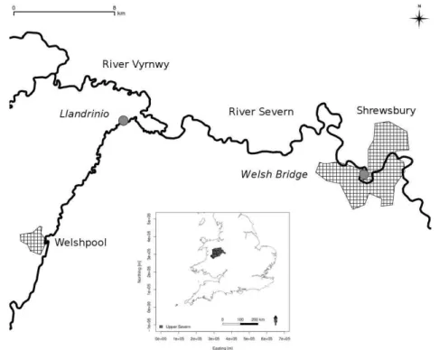
Fig. 1.Schematic map showing the upper River and Vyrnwy tributary which both flow from west to east. Gauged locations considered in the study (circles) and urban areas are shown (hatched). The insert shows the location of the catchment within the UK.

(Todini, 2008) and much higher during recession periods. Residuals in extreme situations, such as floods may also pos-sess characteristics different to the majority of the data. Fur-thermore, each flood may reveal previously unknown short-comings in the hydrological/hydraulic model(s) making their residuals difficult to predict. In such situations, it may be use-ful to utilise robust error models and predictive bounds (e.g. Rougier et al., 2009; Vernon et al., 2010).

This paper considers the use of DA to improve the fore-casts of the difference between the output of a determinis-tic hydrological model and the observed data. It explores the use of a multiplicative gain to correct the deterministic fore-casts. This gain is evolved stochastically. Forecasts of future observed values, that is futureyt, are expressed as

probabil-ity distributions dependent upon both the gain and the de-terministic forecast of the hydrological model. The approach presented has been utilised previously for operational flood forecasting (Lees et al., 1994). This paper extends previous work by considering a broader family of models for the evo-lution of the gain and two contrasting parameter estimation techniques.

Section 2 outlines the error model for providing proba-bilistic forecasts at a single observational site. In doing so a family of parsimonious models for the evolution of the gain are introduced. The use of the linear Kalman filter for DA and generation of predictive distributions is presented. Meth-ods for estimating the parameters of the model are discussed in Sect. 3. Section 4 presents an example application using an

operational flood forecasting model from the UK. The valid-ity of the assumptions used in parameter estimation is inves-tigated and the usefulness of the uncertainty representations illustrated.

2 Methodology

This section presents the stochastic error model utilised within this paper and the computation of the predictive distri-bution. The representation of the stochastic error model and its evolution is outlined in a state space framework giving a natural framework for computing the predictive distribution as a filtering problem.

2.1 Error model

Recall thaty1:T =(y1, . . . , yT)is a vector ofT observations

indexed by time with corresponding deterministic hydrolog-ical/hydraulic model predictionsm1:T. The observationytis

then related to the predictionmt by an adaptive gaingt and

noise termǫt as outlined in Eq. (3).

yt =mtgt+ǫt (3)

The gaingt is a time varying correction for the bias in the

(4)

Fig. 2.Summary plots of the data available for Welsh bridge during the calibration period. Points represent observed data with the line being the concatenation of the output of the most recent hydraulic model initialisation. A bias in the prediction of low flows is clearly shown as are periods of missing data and poor model initialisation.

such as autoregressive moving average processes could also be considered.

The simplest local level model considered is a random walk wheregt is given as the sum of its previous value and

the stochastic noiseηt. That is

gt=gt−1+ηt. (4)

This is referred to as the random walk (RW) model. The local linear trend (LLT) model generalises this by introducing the slopedt which follows a random walk driven by the

stochas-tic noiseξt. Thus,

gt =gt−1+dt−1+ηt (5)

dt =dt−1+ξt. (6)

In this paper it is assumed thatǫt, along with the stochastic

noise termsηt andξt, are not correlated with each other or in

time. Further, they are realisations of unimodal, symmetric, unbounded random variables that can be summarised by their first two moments which are defined using the parametersσ2, qηandqξas

E [ǫt]=E [ηt]=E [ξt]=0

Var [ǫt]=σ2

Var [ηt]=qησ2

Var [ξt]=qξσ2.

The validity of these assumptions can be assessed from the forecast residuals as shown in Sect. 4. Two methods for es-timation of the parameters are presented in Sect. 3.

Three further local level models can be specified by plac-ing constraints on the LLT model. Ifqη=qξ, the trend in the

LLT model is deterministic, resulting in the deterministic lo-cal linear trend (DLLT) model. Whenqξ is zero, the slope is

fixed and the evolution of the gain becomes a random walk with drift (RWD) model, that is

gt=gt−1+d+ηt.

Settingqηto zero but allowing positiveqξ results in an

in-tegrated random walk trend, referred to as the IRW model. This often results in a smoother adaptation ofgtcompared to

the RW model outlined in Eq. (4).

The models outlined above forgt are parsimonious, the

only unknown parameters other thanσ2being the values of noise variance ratiosqηandqξ. A further level of complexity

can be included by incorporating smoothing or damping pa-rameters. Inclusion of such a parameterαin Eq. (4) results in a first order auto regressive (AR) model for the gain:

gt=αgt−1+ηt. (7)

Inclusion of the smoothing parameters (αandβ) in the local linear trend model gives

gt =αgt−1+dt−1+ηt (8)

dt =βdt−1+ξt. (9)

This is referred to as the smoothed local linear trend (SLLT) model. Two special cases of this are the smoothed ran-dom walk (SRW) model; in whichβ=1 and qη=0; and

the damped trend (DT) model in whichqη=qξ andα=1.

(5)

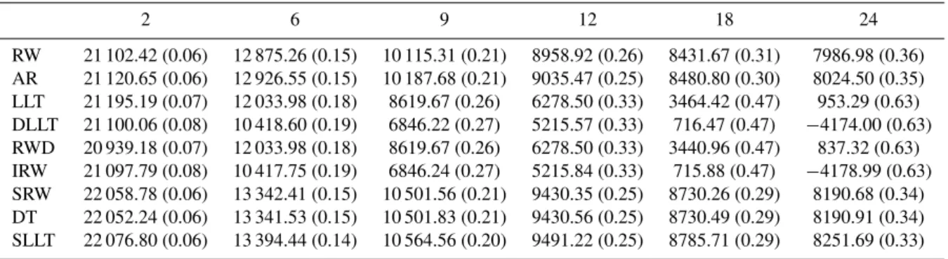
Table 2.Calibration results for Welsh bridge showing the log likelihood and RMSE (bracketed) for various forecast lead times (hours) and GRW models.

2 6 9 12 18 24

RW 21 102.42 (0.06) 12 875.26 (0.15) 10 115.31 (0.21) 8958.92 (0.26) 8431.67 (0.31) 7986.98 (0.36) AR 21 120.65 (0.06) 12 926.55 (0.15) 10 187.68 (0.21) 9035.47 (0.25) 8480.80 (0.30) 8024.50 (0.35) LLT 21 195.19 (0.07) 12 033.98 (0.18) 8619.67 (0.26) 6278.50 (0.33) 3464.42 (0.47) 953.29 (0.63) DLLT 21 100.06 (0.08) 10 418.60 (0.19) 6846.22 (0.27) 5215.57 (0.33) 716.47 (0.47) −4174.00 (0.63) RWD 20 939.18 (0.07) 12 033.98 (0.18) 8619.67 (0.26) 6278.50 (0.33) 3440.96 (0.47) 837.32 (0.63) IRW 21 097.79 (0.08) 10 417.75 (0.19) 6846.24 (0.27) 5215.84 (0.33) 715.88 (0.47) −4178.99 (0.63) SRW 22 058.78 (0.06) 13 342.41 (0.15) 10 501.56 (0.21) 9430.35 (0.25) 8730.26 (0.29) 8190.68 (0.34) DT 22 052.24 (0.06) 13 341.53 (0.15) 10 501.83 (0.21) 9430.56 (0.25) 8730.49 (0.29) 8190.91 (0.34) SLLT 22 076.80 (0.06) 13 394.44 (0.14) 10 564.56 (0.20) 9491.22 (0.25) 8785.71 (0.29) 8251.69 (0.33)

2.2 State Space form

All the models outlined can be conveniently expressed in a state space form with state vectorxt=gt dt′ describing

the gain (gt) and its slope (dt). The state vector evolves

ac-cording the state transition matrixFand system noise matrix Gas

xt=Fxt−1+G

ηt

ξt

. (10)

The state vector is related to the observations by

yt=h′txt+ǫt (11)

whereht=mt 0′. The values taken byFandGdepend

upon the local level model selected. Table 1 outlines the val-ues taken in terms of the matrix forms given in Eq. (12) for the various models considered along with any other parame-ter constraints.

F=

F11F12 0 F22

G=

G11 0 0 G22

. (12)

Two methods for the estimation of the parameters are pre-sented in Sect. 3. The following sub-section discusses the use of the Kalman filter to generate the expected value and co-variance of the predictive distributions.

2.3 Prediction using the Kalman filter

The assumptions regarding the stochastic noise terms pre-sented in Sect. 2.1 are the minimum required for application of the linear Kalman filter (Kalman, 1960). Suppose the dis-tribution ofxt has similar properties to that of the stochastic

noise terms with its expected value and variance given by ˆ

xt andσ2Pt. (wherePt is a 2×2 matrix), respectively. The

Kalman filter can be used to predict future states and assimi-late the observed data as it becomes available.

The one step ahead predictions of the distribution of the states, conditional upon the data up to timet, are given by the expected value:

ˆ

xt+1|t =Fxˆt|t (13)

and varianceσ2Pt+1|t where

Pt+1|t =FPt|tF′+GQG′. (14)

The noise variance ratio matrixQis constructed as

Q=

qη 0

0 qξ

.

Thef-step ahead prediction of the states given the informa-tion up to timet can be computed by repeated application of Eqs. (13) and (14).

The f-step ahead prediction error νt+f|t and prediction

varianceσ2ψt+f|tcan be computed from the forecast states

using:

νt+f|t =yt+f−h′t+fxˆt+f|t (15)

ψt+f|t =1+h′t+fPt+f|tht+f (16)

Evaluation of these expressions requires knowledge of the future predictions of the flood forecasting model.

When a new observation becomes available it can be used to condition the distribution of the gain by updating the mean and covariance of the one step ahead prediction of the state distribution using Eqs. (17) to (19) (see for example Kalman, 1960, for a derivation).

kt+1=Pt+1|tht+1ψ_t−₊1₁_|_t (17) ˆ

xt+1|t+1= ˆxt+1|t +kt+1νt+1|t (18) Pt+1|t+1 =Pt+1|t −kt+1h′t+1Pt+1|t (19)

To evaluate the above recursions some initial values for ˆ

(6)

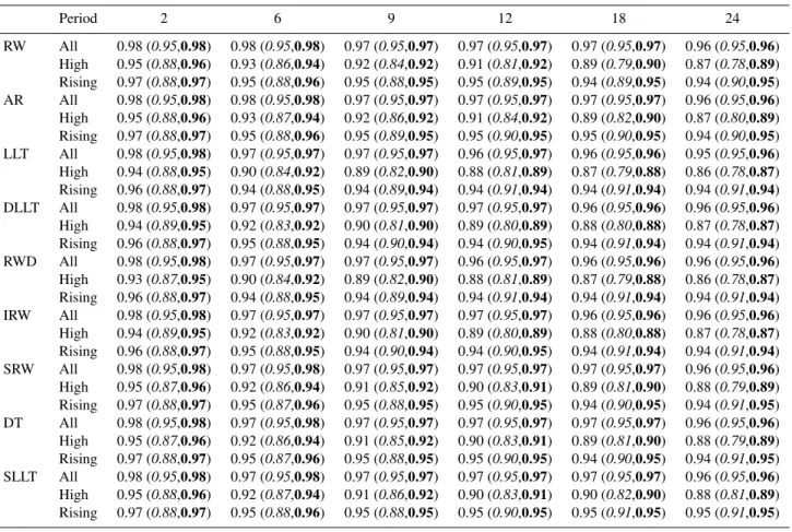
Table 3.Fraction of observations at Welsh bridge bracketed by the estimated 95 % prediction intervals during calibration. Bracketed results are those for the SEFE calibration with the italicised and bold values corresponding to the empirical and theoretical symmetric bounds. Results are shown for all the time periods, high levels (>2m) and periods where the hydrograph is rising for different combinations of lead time (hours) and GRW model.

Period 2 6 9 12 18 24

RW All 0.98 (0.95,0.98) 0.98 (0.95,0.98) 0.97 (0.95,0.97) 0.97 (0.95,0.97) 0.97 (0.95,0.97) 0.96 (0.95,0.96) High 0.95 (0.88,0.96) 0.93 (0.86,0.94) 0.92 (0.84,0.92) 0.91 (0.81,0.92) 0.89 (0.79,0.90) 0.87 (0.78,0.89) Rising 0.97 (0.88,0.97) 0.95 (0.88,0.96) 0.95 (0.88,0.95) 0.95 (0.89,0.95) 0.94 (0.89,0.95) 0.94 (0.90,0.95) AR All 0.98 (0.95,0.98) 0.98 (0.95,0.98) 0.97 (0.95,0.97) 0.97 (0.95,0.97) 0.97 (0.95,0.97) 0.96 (0.95,0.96) High 0.95 (0.88,0.96) 0.93 (0.87,0.94) 0.92 (0.86,0.92) 0.91 (0.84,0.92) 0.89 (0.82,0.90) 0.87 (0.80,0.89) Rising 0.97 (0.88,0.97) 0.95 (0.88,0.96) 0.95 (0.89,0.95) 0.95 (0.90,0.95) 0.95 (0.90,0.95) 0.94 (0.90,0.95) LLT All 0.98 (0.95,0.98) 0.97 (0.95,0.97) 0.97 (0.95,0.97) 0.96 (0.95,0.97) 0.96 (0.95,0.96) 0.95 (0.95,0.96) High 0.94 (0.88,0.95) 0.90 (0.84,0.92) 0.89 (0.82,0.90) 0.88 (0.81,0.89) 0.87 (0.79,0.88) 0.86 (0.78,0.87) Rising 0.96 (0.88,0.97) 0.94 (0.88,0.95) 0.94 (0.89,0.94) 0.94 (0.91,0.94) 0.94 (0.91,0.94) 0.94 (0.91,0.94) DLLT All 0.98 (0.95,0.98) 0.97 (0.95,0.97) 0.97 (0.95,0.97) 0.97 (0.95,0.97) 0.96 (0.95,0.96) 0.96 (0.95,0.96) High 0.94 (0.89,0.95) 0.92 (0.83,0.92) 0.90 (0.81,0.90) 0.89 (0.80,0.89) 0.88 (0.80,0.88) 0.87 (0.78,0.87) Rising 0.96 (0.88,0.97) 0.95 (0.88,0.95) 0.94 (0.90,0.94) 0.94 (0.90,0.95) 0.94 (0.91,0.94) 0.94 (0.91,0.94) RWD All 0.98 (0.95,0.98) 0.97 (0.95,0.97) 0.97 (0.95,0.97) 0.96 (0.95,0.97) 0.96 (0.95,0.96) 0.96 (0.95,0.96) High 0.93 (0.87,0.95) 0.90 (0.84,0.92) 0.89 (0.82,0.90) 0.88 (0.81,0.89) 0.87 (0.79,0.88) 0.86 (0.78,0.87) Rising 0.96 (0.88,0.97) 0.94 (0.88,0.95) 0.94 (0.89,0.94) 0.94 (0.91,0.94) 0.94 (0.91,0.94) 0.94 (0.91,0.94) IRW All 0.98 (0.95,0.98) 0.97 (0.95,0.97) 0.97 (0.95,0.97) 0.97 (0.95,0.97) 0.96 (0.95,0.96) 0.96 (0.95,0.96) High 0.94 (0.89,0.95) 0.92 (0.83,0.92) 0.90 (0.81,0.90) 0.89 (0.80,0.89) 0.88 (0.80,0.88) 0.87 (0.78,0.87) Rising 0.96 (0.88,0.97) 0.95 (0.88,0.95) 0.94 (0.90,0.94) 0.94 (0.90,0.95) 0.94 (0.91,0.94) 0.94 (0.91,0.94) SRW All 0.98 (0.95,0.98) 0.97 (0.95,0.98) 0.97 (0.95,0.97) 0.97 (0.95,0.97) 0.97 (0.95,0.97) 0.96 (0.95,0.96) High 0.95 (0.87,0.96) 0.92 (0.86,0.94) 0.91 (0.85,0.92) 0.90 (0.83,0.91) 0.89 (0.81,0.90) 0.88 (0.79,0.89) Rising 0.97 (0.88,0.97) 0.95 (0.87,0.96) 0.95 (0.88,0.95) 0.95 (0.90,0.95) 0.94 (0.90,0.95) 0.94 (0.91,0.95) DT All 0.98 (0.95,0.98) 0.97 (0.95,0.98) 0.97 (0.95,0.97) 0.97 (0.95,0.97) 0.97 (0.95,0.97) 0.96 (0.95,0.96) High 0.95 (0.87,0.96) 0.92 (0.86,0.94) 0.91 (0.85,0.92) 0.90 (0.83,0.91) 0.89 (0.81,0.90) 0.88 (0.79,0.89) Rising 0.97 (0.88,0.97) 0.95 (0.87,0.96) 0.95 (0.88,0.95) 0.95 (0.90,0.95) 0.94 (0.90,0.95) 0.94 (0.91,0.95) SLLT All 0.98 (0.95,0.98) 0.97 (0.95,0.98) 0.97 (0.95,0.97) 0.97 (0.95,0.97) 0.97 (0.95,0.97) 0.96 (0.95,0.96) High 0.95 (0.88,0.96) 0.92 (0.87,0.94) 0.91 (0.86,0.92) 0.90 (0.83,0.91) 0.90 (0.82,0.90) 0.88 (0.81,0.89) Rising 0.97 (0.88,0.97) 0.95 (0.88,0.96) 0.95 (0.88,0.95) 0.95 (0.90,0.95) 0.95 (0.91,0.95) 0.95 (0.91,0.95)

3 Estimation

This section discusses the estimation of the unknown pa-rameter vectorθ defined for the models considered in Ta-ble 1. Two estimation techniques are outlined and there re-sults contrasted in Sect. 4. The first technique is maximum likelihood estimation based upon the assumption that the pre-diction errors are independent realisations of Gaussian ran-dom variables. This introduces stronger assumptions about the stochastic noise terms than those introduced in Sect. 2.1. The second method which is based on minimising the sum of the squared expected forecast errors, is more heuristic. In both cases the validity of the error assumptions can be as-sessed. This is discussed along with the the construction of predictive error bounds.

3.1 Gaussian maximum likelihood

In Gaussian maximum likelihood (GML) estimation, the pa-rametersθare estimated by maximising the likelihood of the f-step ahead predictions when it is believed that νt+f|t is

drawn independently from a zero mean Gaussian

distribu-tion with variance σ2ψt+f|t. Under these assumptions the

log likelihood is

l (θ )=K−1 2

T−f X

t=t0

logσ2ψt+f|t

− 1 2σ2

T−f X

t=t0

ν_t2₊_f_|_tψ_t−₊1_f_|_t (20)

whereKis a constant with respect toθ. The maximum like-lihood estimate ofσ2can be computed conditional upon the other parameters inθas

ˆ

σ2= 1 T −f−t0

T−n X

t=t0

ν_t2₊_f_|_tψ_t−₊1_f_|_t. (21)

This allows σ2 to be concentrated out of Eq. (20) leaving (Schweppe, 1965):

lθ\σ2=K−1 2

T−f X

t=t0

logσˆ2ψt+f|t

(7)

Table 4. Precision of the forecasts (see text for definition) during calibration at Welsh bridge. Bracketed results are those for the SEFE calibration with the italicised and bold values corresponding to the empirical and theoretical symmetric bounds. Results are shown for all the time periods, high levels (>2 m) and periods where the hydrograph is rising for different combinations of lead time (hours) and GRW model.

Period 2 6 9 12 18 24

which is dependent upon the remaining parameters (denoted θ\σ2_{). This can be numerically optimised to give maximum} likelihood parameter estimates ofθ.

The uncertainty in the predictions can be expressed as per-centile confidence intervals for the predictions constructed as:

h′_t₊_fxˆt+f|t ±κpσ ψˆ 1 2

t+f|t (23)

wereκpis constant dependent uponpand can be computed

from a standard normal distribution; for exampleκ95≈1.96. The normality of the forecast residuals and their correla-tion can be readily assessed using, for example, quantile and auto correlation plots (Box and Jenkins, 1994).

3.2 Minimising the sum of the squared expected forecast errors

The second estimation technique, referred to as SEFE for the remainder of this paper, is based on the appeal of minimising

the sum of the squared expected forecasting error:

Sf = T−f

X

t=t0

ν_t2₊_f_|_t. (24)

This ensures that the expected value of the forecast is as close as possible (in terms of average squared error) to the ob-served data. The minimisation ofSf allows the estimation

of all the parameters inθexceptσ2. A value forσ2can then be estimated using Eq. (21) if required. The error assump-tions of the Kalman filter (Sect. 2.1) imply that each pre-dictive distribution is uni-modal, symmetric and unbounded. Testing the symmetry of the forecast residuals, for example using Wilcoxon sign rank test (Wilcoxon, 1945), can indi-cate if this assumption is valid. Two methods for construction of predictive confidence intervals are considered. They make use of the theoretical symmetry of the forecast distribution and result in symmetric prediction intervals.

The symmetry of the forecast distribution implies that pre-diction confidence intervals can be expressed as

h′t+fxˆt+f|t ±ρpψ 1 2

(8)

Fig. 3.Summary plots of the analysis of the 6 h forecast residuals at Welsh Bridge for the DT model calibrated using the Gaussian maximum likelihood methodology. The upper pane shows the quantile-quantile plot of the standardised residuals compared to a standard normal distribution. The lower pane shows the auto-correlation of the residuals.

The values of ρp can be estimated empirically as the pth

percentile of

νt+f|tψ −1

2 t+f|t

. Given the finite population of

residuals, this empirical estimate ofρpmay not be not robust

at high values of p. The values of ρp can be adapted (for

givenp) as more data becomes available. Sequential tests for symmetry (e.g. Weed and Bradley, 1971) may be of use in such situations.

Pukelsheim (1994) gives theoretical results for the upper limits ofρpunder the uni-model, symmetric and unbounded

distributional assumptions. Specifically

Pr



 

yt−µt+f|t

ψ− 1 2 t+f|t

≥r



 ≤

4σ2

9r2 r >1.63σ. (26)

The caser=3σis the three sigma rule; that there is less than 5 % probability of a sample from univariate random variable random with the aforementioned properties being outside of 3 standard deviations from the mean. These upper limits can be used in two ways. Firstly, they allow for the estimation of conservative prediction confidence intervals, allowing for a more cautious view to be taken of the prediction uncertainty. The second use is as a means of analysing the suitability of the adaptive gain models considered by contrasting the

sym-metrical empirical estimates and the theoretic upper limits for a givenp.

4 Upper Severn case study

To illustrate the effectiveness and limitations of the proposed methodology in an operational setting a case study based on the upper Severn catchment (UK) is presented. The upper Severn river network is situated on the border of England and Wales and shown in Fig. 1. The River Severn rises in the Cambrian mountains (741 mAOD) and flows to the north-east before meeting the Vyrnwy tributary at Crew Green. The valley is wide and flat in this confluence area, with a considerable extent of flood plain. The river then flows east to Shrewsbury. The lower boundary of the 2284 km2upper Severn catchment is defined by the gauge at Welsh bridge in Shrewsbury where the median annual flood is greater than 284 cumecs. Average annual rainfall can exceed 2500 mm in the head waters of the catchment. The catchment has seen seven significant flood events in the past twelve years.

(9)

Fig. 4.Summary plots of the analysis of the 6 h forecast residuals for the RW model calibrated using the SEFE methodology. The upper pane shows the cumulative distributions of the absolute values of the residuals at Welsh Bridge. The solid line being positive residuals and the dotted line being negative residuals. The lower pane shows the auto-correlation of the residuals.

of the catchment and Llandrinio an internal node of the hy-draulic model at which observations are available. The latter is just upstream of the junction with the major Vyrnwy tribu-tary and may be affected by backwater effects at flood stages. At both sites water levels are observed every 15 min.

Operationally, the flood forecasting model is run with a 15 minute time step and evaluated twice daily. At midnight it is run in a continuous mode using observed inputs and output data assimilation to generate a set of “warm states” which are used to initialise the forecasts. The first set of forecasts issued at midnight (00:00) give up to 36 h lead time using forecast precipitation. The second set of forecasts is issued at mid-day (12:00). These forecasts are initialised by evolving the “warm states” using the observed meteorological variables between midnight and midday. Forecast precipitation is then used to evaluate the flood forecasting model giving forecasts of the hydrological variables with up to 36 h lead time. Fur-ther details can be found in Weerts et al. (2011).

The adaptive gain correction is initialised at the start of each forecast period. The first four hours of forecasts are used as a burn-in period for the adaptive gain. Then, in keeping with the operational system, forecasts are issued based on the most recent forecast run of the flood forecasting model for which the adaptive gain is burnt in. A single year of data (2006) which contains a significant flood event is used to identify and estimate the adaptive correction. Three years

(2007–2009) are used for validation purposes. The results for each of the sites are summarised below.

4.1 Welsh bridge

Figure 2 shows the hydraulic model predictions and observed data at Welsh bridge during the calibration period. There is a systematic over estimation of the water level during periods of low flow. Such a systematic bias may arise from the cal-ibration of the hydraulic model. If the model was calibrated to discharge data and the representation of the gauged cross section poor at shallow depths, such a bias may result. Alter-natively an artificially high low water level within the model, such as that seen here, can arise as a means of achieving ac-ceptable representations of high water level periods.

(10)

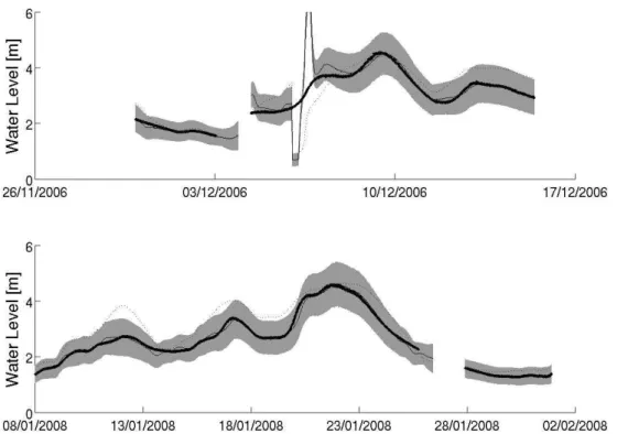
Fig. 5.Examples of 6 h ahead forecasts given at Welsh bridge for two large flood events during calibration (upper pane) and validation (lower pane) periods generated using the SLLT model calibrated using the Guassian methodology. The shaded area represents the 95 % prediction confidence interval with the solid line being the expected value of the predictions. Observed data points are also shown along with the deterministic model forecast (dotted line).

(11)

Table 5.Fraction of observations at Welsh bridge bracketed by the estimated 95 % prediction intervals during validation. Bracketed results are those for the SEFE calibration with the italicised and bold values corresponding to the empirical and theoretical symmetric bounds. Results are shown for all the time periods, high levels (>2 m) and periods where the hydrograph is rising for different combinations of lead time (hours) and GRW model.

Period 2 6 9 12 18 24

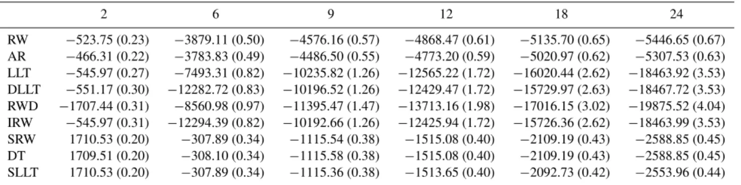
Table 6.Calibration results for Llandrinio showing the log likelihood and RMSE (bracketed) for various forecast lead times (hours) and GRW models.

2 6 9 12 18 24

RW −523.75 (0.23) −3879.11 (0.50) −4576.16 (0.57) −4868.47 (0.61) −5135.70 (0.65) −5446.65 (0.67) AR −466.31 (0.22) −3783.83 (0.49) −4486.50 (0.55) −4773.20 (0.59) −5020.97 (0.62) −5307.53 (0.63) LLT −545.97 (0.27) −7493.31 (0.82) −10235.82 (1.26) −12565.22 (1.72) −16020.44 (2.62) −18463.92 (3.53) DLLT −551.17 (0.30) −12282.72 (0.83) −10196.52 (1.26) −12429.47 (1.72) −15729.97 (2.63) −18467.72 (3.53) RWD −1707.44 (0.31) −8560.98 (0.97) −11395.47 (1.47) −13713.16 (1.98) −17016.15 (3.02) −19875.52 (4.04) IRW −545.97 (0.31) −12294.39 (0.82) −10192.66 (1.26) −12425.94 (1.72) −15726.36 (2.62) −18463.99 (3.53) SRW 1710.53 (0.20) −307.89 (0.34) −1115.54 (0.38) −1515.08 (0.40) −2109.19 (0.43) −2588.85 (0.45) DT 1709.51 (0.20) −308.10 (0.34) −1115.58 (0.38) −1515.08 (0.40) −2109.19 (0.43) −2588.85 (0.45) SLLT 1710.53 (0.20) −307.89 (0.34) −1115.36 (0.38) −1513.65 (0.40) −2092.73 (0.42) −2553.96 (0.44)

Table 2 presents the log likelihood and root mean squared error (RMSE) summaries of the calibration results at various forecast lead times. For both calibration methodologies, the performance of the LLT model along with its special cases DLLT, RWD and IRW decays much more rapidly with lead time than the alternative models. This suggests that as with the SLLT, SRW and DT models there is the need to recognise

(12)

Fig. 7.Examples of 6 h ahead forecasts given at Llanrinio for two large flood events during calibration (upper pane) and validation (lower pane) periods generated using the SLLT model calibrated using the SEFE methodology with empirical error bounds. The shaded area represents the 95 % prediction confidence interval with the solid line being the expected value of the predictions. Observed data points are also shown along with the deterministic model forecast (dotted line).

Calibration with the GML methodology allows model se-lection to be performed using time series identification crite-ria, such as the AIC (Akaike, 1974) or BIC (Schwarz, 1978). This leads to the selection of the SLLT at all the lead times considered. The RMSE results of the SEFE calibration sug-gest that at shorter lead times, a more parsimonious model, such as the RW, may be suitable. Further analysis of the pre-dictive performance of the models can be gained by examin-ing the coverage and precision of the forecasts shown for the calibration period in Tables 3 and 4.

Table 3 shows the percentage of points falling within the 95 % prediction confidence interval for various lead times during calibration. Results are shown for three categories: the whole period, high water levels greater than 2 m and rising parts of the observed hydrograph whereyt+1> yt. By

defi-nition the empirical bounds derived from the SEFE method-ology bracket 95 % of all the (calibration) observations. Cov-erage of the high and rising flow categories for this method-ology is less than 95 % for all models and lead times. Cover-age of high flows decreases with increasing lead time for all the models. This indicates that the pooling of the residuals in computing the empirical bounds may not be appropriate. The values ofκp, or indeed the model parameters, may be state

or time dependent (Young, 2002; Young et al., 2001). The theoretical prediction bounds of the SEFE methodol-ogy give in all cases percentages of coverage based on all the

calibration data that is consistent with the error assumptions outlined in Sect. 2.1. A similar pattern to the empirical re-sults for the coverage of the high and rising flows categories is shown.

The high percentages for coverage when using the Gaus-sian likelihood calibration at short forecast lead times sup-port the suggestion that the assumptions used in deriving the likelihood may not be valid. However, at lead times up to six hours, there is less evidence of systematic differences in the percentage of observations covered in the three discharge categories. As with the SEFE calibration at longer lead times, the coverage of the high flow category deteriorates for all the models.

The results in Tables 4 summarise the precision of the of the forecasts through the mean of the forecasts standard deviation over each flow category. The empirically derived forecast error bounds are, especially at lead times up to six hours, significantly sharper than the theoretical upper limit and those resulting from the Gaussian calibration.

Figure 3 shows two summary plots of the standardised 6 h forecast residuals of the SLLT model calibrated us-ing the Gaussian likelihood methodology. The upper pane shows a quantile-quantile plot of the standardised residual νt+f|tσˆ−1ψ

−1 2

t+f|t against a standard norm distribution. The

(13)

Table 7.Fraction of observations at Llandrinio bracketed by the estimated 95 % prediction intervals during calibration. Bracketed results are those for the SEFE calibration with the italicised and bold values corresponding to the empirical and theoretical symmetric bounds. Results are shown for all the time period, high levels (>4 m) and periods where the hydrograph is rising for different combinations of lead time (hours) and GRW model.

Period 2 6 9 12 18 24

valid. The residual distribution is approximately symmetric. Therefore, the use of the Kalman filter may be a valid approx-imation, even if the resulting prediction confidence intervals are not appropriately defined. The lower plot indicates that the residuals are correlated up to at least a lag of 28 samples, or 7 h, approximately the forecast lead time. This and the low correlation value suggest that the conditional independence assumption, while not strictly valid, may be a reasonable ap-proximation.

The forecast residuals of the SEFE methodology can also be assessed. The lower pane of Fig. 4 shows the auto-correlation pattern in the residuals of the RW model fitted by the SEFE methodology for a 6 h leadtime. The correlation within the residuals lower and less persistent at longer lags than for the Gaussian calibration. The upper pane of Fig. 4 shows the cumulative distributions of the positive standard-ised residuals along with that of the absolute value of nega-tive standardised residuals. It indicates a lack of symmetry in the residuals confirmed by a Wilcoxon sign rank test.

Table 5 shows the percentage of observations falling within the 95 % prediction confidence interval during the

val-idation period. The high percentages for the GML methodol-ogy further support the suggestion that the assumptions used in deriving the likelihood may not be valid. The results for the SEFE calibration indicate that the symmetrical empiri-cal estimation ofρpderived during calibration perform well

in the validation period. The predictive bounds derived us-ing the theoretical upper limit appear to bracket around 99 % of the data during the validation period, suggesting they are unduly conservative.

Figure 5 shows the predictions made using the SLLT model calibrated using the Gaussian methodology for the largest flood events at Welsh bridge in the calibration and val-idation periods. The results are encouraging with the adap-tive gain acting to correct the model forecast towards the ob-served values. During both the calibration and validation pe-riod adaptive gain methodology is able to correct for errors in both the timing and magnitude of the hydrograph peaks as well as the receding limb.

(14)

Table 8. Precision of the forecasts (see text for definition) during calibration at Llandrinio. Bracketed results are those for the SEFE calibration with the italicised and bold values corresponding to the empirical and theoretical symmetric bounds. Results are shown for all the time period, high levels (>4 m) and periods where the hydrograph is rising for different combinations of lead time (hours) and GRW model.

Period 2 6 9 12 18 24

RW All 0.74 (0.13,1.24) 1.03 (0.39,1.56) 1.09 (0.51,1.66) 1.11 (0.61,1.68) 1.12 (0.70,1.70) 1.13 (0.71,1.72) High 1.00 (0.27,2.53) 1.51 (0.59,2.38) 1.68 (0.81,2.62) 1.77 (0.99,2.76) 1.87 (1.22,2.93) 1.96 (1.27,3.09) Rising 0.76 (0.14,1.33) 1.07 (0.40,1.63) 1.14 (0.54,1.74) 1.16 (0.64,1.77) 1.18 (0.75,1.80) 1.20 (0.76,1.84) AR All 0.73 (0.13,1.24) 1.02 (0.43,1.56) 1.08 (0.53,1.66) 1.10 (0.60,1.69) 1.11 (0.70,1.72) 1.12 (0.74,1.74) High 0.99 (0.27,2.52) 1.49 (0.64,2.36) 1.65 (0.83,2.61) 1.74 (0.97,2.75) 1.84 (1.19,2.94) 1.92 (1.32,3.10) Rising 0.75 (0.14,1.33) 1.06 (0.44,1.63) 1.13 (0.56,1.74) 1.15 (0.63,1.78) 1.17 (0.74,1.82) 1.19 (0.79,1.86) LLT All 0.86 (0.11,1.72) 1.83 (0.78,3.02) 2.64 (1.24,4.43) 3.31 (1.67,5.75) 4.55 (2.37,8.15) 6.77 (3.09,11.21)

High 1.01 (0.23,3.49) 2.83 (1.11,4.32) 4.11 (1.82,6.49) 5.64 (2.68,9.22) 8.96 (4.56,15.67) 13.68 (6.22,22.56) Rising 0.90 (0.12,1.84) 2.01 (0.85,3.31) 3.18 (1.52,5.40) 4.20 (2.19,7.52) 5.99 (3.30,11.35) 9.35 (4.35,15.76) DLLT All 0.86 (0.10,1.90) 2.47 (0.78,3.02) 2.72 (1.24,4.41) 3.51 (1.67,5.72) 4.98 (2.36,8.12) 6.77 (3.08,11.16) High 1.01 (0.19,3.60) 4.55 (1.11,4.32) 4.14 (1.82,6.48) 5.79 (2.68,9.20) 9.67 (4.55,15.62) 13.69 (6.20,22.46) Rising 0.90 (0.11,2.02) 2.69 (0.85,3.31) 3.29 (1.51,5.37) 4.54 (2.18,7.49) 6.83 (3.29,11.30) 9.35 (4.33,15.68) RWD All 0.92 (0.18,1.43) 2.05 (0.87,3.39) 2.90 (1.39,5.11) 3.80 (1.87,6.92) 5.35 (2.86,10.48) 7.53 (4.01,15.37) High 1.22 (0.37,2.93) 3.29 (1.31,5.10) 4.77 (2.10,7.69) 6.62 (3.02,11.15) 10.66 (5.49,20.09) 15.47 (8.05,30.83) Rising 0.97 (0.20,1.54) 2.25 (0.95,3.71) 3.45 (1.70,6.22) 4.82 (2.46,9.09) 7.15 (4.07,14.90) 10.24 (5.81,22.24) IRW All 0.86 (0.10,1.93) 2.47 (0.78,3.02) 2.72 (1.24,4.41) 3.51 (1.66,5.72) 4.98 (2.37,8.11) 6.77 (3.08,11.15)

High 1.01 (0.19,3.58) 4.55 (1.11,4.32) 4.14 (1.82,6.48) 5.79 (2.67,9.19) 9.66 (4.55,15.60) 13.68 (6.20,22.44) Rising 0.90 (0.11,2.05) 2.69 (0.85,3.31) 3.29 (1.51,5.37) 4.54 (2.18,7.48) 6.82 (3.29,11.29) 9.34 (4.32,15.66) SRW All 0.66 (0.10,1.29) 0.88 (0.52,1.36) 1.02 (0.73,1.57) 1.11 (0.91,1.71) 1.25 (1.14,1.93) 1.43 (1.35,2.22)

High 0.71 (0.20,2.51) 0.97 (0.60,1.57) 1.10 (0.84,1.80) 1.23 (1.07,2.02) 1.60 (1.55,2.63) 1.97 (1.96,3.23) Rising 0.67 (0.11,1.38) 0.91 (0.54,1.42) 1.10 (0.80,1.72) 1.26 (1.05,1.97) 1.50 (1.39,2.36) 1.77 (1.71,2.80) DT All 0.66 (0.10,1.29) 0.88 (0.52,1.36) 1.02 (0.73,1.57) 1.11 (0.91,1.71) 1.25 (1.14,1.93) 1.43 (1.35,2.22) High 0.71 (0.21,2.55) 0.97 (0.60,1.57) 1.10 (0.84,1.80) 1.23 (1.07,2.02) 1.60 (1.55,2.63) 1.97 (1.96,3.23) Rising 0.67 (0.11,1.38) 0.91 (0.54,1.42) 1.10 (0.80,1.72) 1.26 (1.05,1.97) 1.50 (1.39,2.36) 1.77 (1.71,2.80) SLLT All 0.66 (0.10,1.29) 0.88 (0.51,1.35) 1.02 (0.72,1.57) 1.11 (0.87,1.71) 1.24 (1.09,1.90) 1.41 (1.29,2.17) High 0.71 (0.21,2.60) 0.97 (0.59,1.55) 1.10 (0.83,1.80) 1.23 (1.04,2.02) 1.59 (1.50,2.62) 1.94 (1.90,3.17) Rising 0.67 (0.11,1.38) 0.91 (0.54,1.40) 1.10 (0.79,1.71) 1.26 (1.00,1.96) 1.49 (1.33,2.31) 1.75 (1.62,2.71)

reveal one aspect of how the adaptive gain behaves in a less than ideal situation. During January there is a period where no observations are taken. During this time, the prediction interval can at first be seen to gradually widen, as no fur-ther observations are available to condition the correction of the current simulation of the flood forecasting model. Then, when the next run of the flood forecasting model becomes available the gain cannot be initialised, so no forecasts are issued. In such situations, the forecaster making operational decisions may wish to consider the past simulation of the flood forecasting model and the corresponding adaptive gain. Figure 6 shows the predictions made for the same event using the RW model calibrated using the SEFE methodology with empirical prediction bounds. Visual comparison with Fig. 5 shows the forecasts to be more precise, but failing to capture the rising limb of the validation hydrograph. 4.2 Llandrinio

Tables 6, 7 and 8 summarise the performance in calibration of the adaptive gain models at Llandrinio. As at Welsh bridge, there is a bias in the baseflow of the hydraulic model. Per-formance is assessed only when the flood forecasting model

predicts a water level greater than 1.8 m. None of the models for the adaptive gain produce a RMSE lower than that of the uncorrected model (0.39) for lead times greater than 9 h. This time is shorter than that at Welsh bridge which is consistent with the location of the gauging site closer to the headwaters of the catchment. As for Welsh bridge the deterioration in performance is more marked for gain models, which include a gradient term but do not include a damping parameter.

The coverage probabilities during calibration (Table 7) are less dependant upon the water level than those at Welsh bridge. In keeping with the Welsh bridge results, the preci-sion of forecasts issued using the SEFE methodology, with empirical error bounds, is higher than that of the gaussian calibration methodology. In validation (9) all the prediction error bounds appear conservative, bracketing a higher pro-portion of the observations than would be expected.

(15)

Table 9.Fraction of observations at Llandrinio bracketed by the estimated 95 % prediction intervals during validation. Bracketed results are those for the SEFE calibration with the italicised and bold values corresponding to the empirical and theoretical symmetric bounds. Results are shown for all the time period, high levels (>4 m) and periods where the hydrograph is rising for different combinations of lead time (hours) and GRW model.

Period 2 6 9 12 18 24

assimilating further observations after initialisation of the gain to improve the precision of the forecasts.

5 Conclusions

The results presented in this paper indicate that compara-tively simple error models combined with real time data as-similation can provide probabilistic forecasts.

Results are shown for a medium size river basin. Two cali-bration methodologies are presented. Detailed residual anal-ysis suggests that, though the error assumptions used in these derivations are not satisfied, they can produce probabilistic forecasts with conservative coverage and precision of the or-der of 10 % of the observed water level. The selection of which calibration methodology performs most adequately re-quires consideration on a case by case basis. Techniques for making this selection are presented.

The lead times at which the expected value of the forecasts can be seem to improve the RMSE of the uncorrected model predictions depends upon the time it takes for the catchment to respond at the gauged site. It remains to be seen if such a

data assimilation methodology is able to perform adequately on small basins where the response to rainfall is more rapid and timing errors, due perhaps to errors in the rainfall fore-cast, are more severe (see Alfieri et al., 2011, for some initial results).

In an operational setting, only the linear Kalman filter evolving two states needs to be evaluated. Though not dis-cussed this can be readily implemented in spreadsheet pack-ages without recourse to more complex programming. This makes the addition of these data assimilation techniques to existing deterministic forecasting systems comparatively straightforward with a very low “cost of entry”.