Robust assessment of future changes in extreme precipitation over the Rhine basin using a GCM

(1)

HESSD

7, 9043–9066, 2010

Future multiday precipitation sums

S. F. Kew et al.

Title Page

Abstract Introduction

Conclusions References

Tables Figures

◭ ◮

Back Close

Full Screen / Esc

Printer-friendly Version Interactive Discussion

Discussion

P

a

per

|

Dis

cussion

P

a

per

|

Discussion

P

a

per

|

Discussio

n

P

a

per

|

Hydrol. Earth Syst. Sci. Discuss., 7, 9043–9066, 2010 www.hydrol-earth-syst-sci-discuss.net/7/9043/2010/ doi:10.5194/hessd-7-9043-2010

Hydrology and Earth System Sciences Discussions

This discussion paper is/has been under review for the journal Hydrology and Earth System Sciences (HESS). Please refer to the corresponding final paper in HESS if available.

Robust assessment of future changes in

extreme precipitation over the Rhine

basin using a GCM

S. F. Kew, F. M. Selten, G. Lenderink, and W. Hazeleger

Royal Netherlands Meteorological Institute, De Bilt, The Netherlands

Received: 3 November 2010 – Accepted: 15 November 2010 – Published: 26 November 2010

Correspondence to: S. F. Kew (sarah.kew@knmi.nl)

(2)

HESSD

7, 9043–9066, 2010

S. F. Kew et al.

Title Page

Tables Figures

◭ ◮

Back Close

Full Screen / Esc

Discussion

P

a

per

|

Dis

cussion

P

a

per

|

Discussion

P

a

per

|

Discussio

n

P

a

per

|

Abstract

Estimates of future changes in extremes of multiday precipitation sums are critical for estimates of future discharge extremes of large river basins. Here we use a large ensemble of global climate model SRES A1b scenario simulations to estimate changes in extremes of 1–20 day precipitation sums over the Rhine basin, projected for the

5

period 2071–2100 with reference to 1961–1990.

We find that in winter, an increase of order 10%, for the 99th percentile precipitation sum, is approximately fixed across the selected range of multiday sums, whereas in summer, the changes become increasingly negative as the summation time lengthens. Explanations for these results are presented that have implications for simple scaling

10

methods for creating time series of a future climate. We show that this scaling be-havior is sensitive to the ensemble size and indicate that currently available discharge estimates from previous studies are based on insufficiently long time series.

1 Introduction

Estimates of future changes in multiday precipitation extremes are critical for estimates

15

of future discharge extremes occuring once every 100–1000 years, yet they are often based on the order of just 30 years of global climate model simulations (Shabalova et al., 2003; Kay et al., 2006; Dankers et al., 2007) or 90 years at best (Lenderink et al., 2007). The precipitation input for discharge models is commonly generated by high resolution regional climate models (RCMs), due to the need to resolve small

20

scale processes. Global climate models (GCMs), however, are required to supply the boundary conditions and effectively impose the large scale flow and its variability on the RCM simulations. If future discharge estimates have been based on too few years of data, there is a risk that the natural variability of the climate has not been adequately sampled (Selten et al., 2004) and the impact of changes in large-scale circulation on

25

(3)

HESSD

7, 9043–9066, 2010

S. F. Kew et al.

Title Page

Tables Figures

◭ ◮

Back Close

Full Screen / Esc

Discussion

P

a

per

|

Dis

cussion

P

a

per

|

Discussion

P

a

per

|

Discussio

n

P

a

per

|

Global warming-induced changes in circulation regimes (e.g. Ulbrich and Christoph, 1999; Gillett et al., 2003; Hu and Wu, 2004; Yin, 2005; Pinto et al., 2007; Brandefelt and K ¨ornich, 2008) and atmospheric moisture content (Trenberth, 1999) are expected to affect the intensity, frequency and relative persistence of extreme precipitation events and dry spells (Frei et al., 2000; Van Ulden and van Oldenborgh, 2006; Van den Hurk et

5

al., 2007; Meehl et al., 2007). In summer, for example, sequences containing long dry spells followed by intense precipitation (Lenderink et al., 2009), might become more common. This could cause multiday precipitation extremes (relevant for catchment-scale discharge) to catchment-scale differently to single-day extremes. That would have implica-tions for the delta-change technique (Lenderink et al., 2007), a method that applies

10

mean changes in climate parameters to transform historical precipitation sequences to future time series for input to hydrological models.

Here we will study changes in extreme multiday precipitation over the Rhine catch-ment area in a very large, 17-member ensemble of the same GCM as in the ESSENCE project (Sterl et al., 2008). With this ensemble we are optimally able to distinguish the

15

climate change signal from natural variability on decadal time scales. The following questions are adressed: How do changes inn-day precipitation extremes depend on

n? Are there significant di_fferences between single-day and multiday precipitation ex-tremes? How large does an ensemble need to be to distinguish climate change from natural variability? The paper is structured as follows: description of the ensemble

20

(Sect. 2), methods (Sect. 3), comparision of GCM results with present-day climate ob-servations (Sect. 4), climate change results (Sect. 5) and concluding remarks (Sect. 6).

2 Study area and data

2.1 The Rhine basin

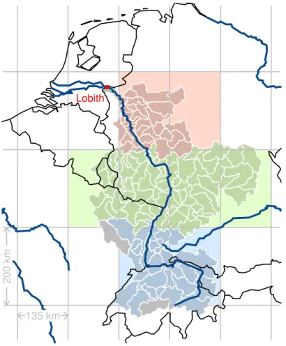
The Rhine basin (Fig. 1) covers an area of 185 000 km2 shared between 9 di_ff

er-25

(4)

HESSD

7, 9043–9066, 2010

S. F. Kew et al.

Title Page

Tables Figures

◭ ◮

Back Close

Full Screen / Esc

Discussion

P

a

per

|

Dis

cussion

P

a

per

|

Discussion

P

a

per

|

Discussio

n

P

a

per

|

length and passes through a range of landscapes, originating in the Swiss Alps, cut-ting through highlands to the North and branching out in several deltas in the Nether-lands before joining the North Sea. The annual mean discharge (1901–2000) at Lobith (Fig. 1) is 2200 m3s−1and current defences are designed to withstand a 1 in 1250-year flood event with a discharge of 16 000 m3s−1_{. It is expected that, as global}

tempera-5

tures rise, the mean discharge of the Rhine will increase in winter, due to increased precipitation and earlier snow melt, and decrease in summer due to reduced precipita-tion and increased evaporaprecipita-tion (e.g. Hurkmans et al., 2010). Such changes will impact the seasonal likelihood of flooding and increase restrictions on river transport in low discharge periods.

10

2.2 ESSENCE data set

The ESSENCE dataset (Sterl et al., 2008) is a 17-member ensemble simulation for the years 1950–2100, generated from the ECHAM5/MPI-OM coupled climate model which has a horizontal resolution of T63 and 31 vertical hybrid atmospheric levels, and is forced by the SRES A1b scenario (Naki´cenovi´c et al., 2000). The di_fferent

15

ensemble members are formed by perturbing the initial state of the atmosphere, with ocean conditions unchanged.

Figure 1 displays the ESSENCE grid over the Rhine basin. There are eight (shaded) ESSENCE grid cells that notably overlap the basin (on the order of 20% or greater of their area is part of the basin) and these are taken to represent the Rhine basin in the

20

ESSENCE data set.

The 8-cell domain representing the Rhine basin is divided into three zonal regions, the North Rhine (2 cells), the Central Rhine (4 cells) and the Alpine Rhine (2 cells), which are treated separately. This choice is motivated by the possible di_fferences in the precipitation distribution following the flow of the river from the south to the north of

25

(5)

HESSD

7, 9043–9066, 2010

S. F. Kew et al.

Title Page

Tables Figures

◭ ◮

Back Close

Full Screen / Esc

Discussion

P

a

per

|

Dis

cussion

P

a

per

|

Discussion

P

a

per

|

Discussio

n

P

a

per

|

domain will also provide multiple output sets for comparison and thus an indication of the consistency of the results and their sensitivity to location.

2.3 CHR-OBS data set

A historical set of precipitation observations issued by the International Commission for the Hydrology of the Rhine basin (CHR) will be used to gauge the model performance.

5

The CHR dataset, recently named CHR-OBS, provides area-averaged daily precipita-tion sums for the 134 Hydrologiska Bry ˚ans Vattenbalansavdelning (HBV) model sub-basins of the Rhine catchment for the period spanning January 1961–December 1995 (Sprokkereef, 2001).

We upscale the CHR data to the approximate size of our chosen regions by

area-10

averaging the daily totals for the group of sub-basins whose centers lie within the boundaries of a particular region (Fig. 1).

3 Methodology

Time series of the area averaged ESSENCE daily precipitation for the three regions are produced for two 30-year time slices: a control period, December 1961–November 1991,

15

and a future period, December 2070–November 2100. A wet-day threshold of 0.1 mm is applied, i.e. values below 0.1 mm are set to zero and thereby treated as dry days. With 17 members, this gives a total of 30×17=510 simulated years for each 30-year

period.

We investigate seasonal differences by comparing results for summer (JJA) and

win-20

(6)

HESSD

7, 9043–9066, 2010

S. F. Kew et al.

Title Page

Tables Figures

◭ ◮

Back Close

Full Screen / Esc

Discussion

P

a

per

|

Dis

cussion

P

a

per

|

Discussion

P

a

per

|

Discussio

n

P

a

per

|

A range of quantiles for each n-day accummulation interval and season are as-sessed. While we focus on the extreme quantiles (q₉₉) of the distribution, we also present results for intermediate quantiles (q₅₀,q₉₀andq₉₅) so that one can gain insight into the robustness of the results. The percentage change of the future precipitation quantile,qf, with respect to the control period quantile,qc, is evaluated i.e.

5

∆q ₌ 100 q

f

− qc

qc !

. (1)

We refer to this relative change as the “scaling”. We determine quantiles for two different distributions:

a. Thefull season of sums including dry events (n-day sum is zero), for which quan-tiles are easily inverted into return values.

10

b. The seasonal distribution excluding dry events, i.e. a multiday equivalent of the

intensity distribution. The term “intensity” is usually used to refer to the mean amount of rainfall on wet days.

For a 10-day sum, method a provides an answer to the question “how much is it likely to rain in a 10-day period in the future compared to now?”. Methodb provides

15

an answer to the question “if it rains at least once in a 10-day period, how much is it likely to rain in the future compared to now?”. In a practical sense, this question might be of importance if an amount of rain exceeding the wet-day threshold is forecast or if current and future 10-day periods with precipitation-favorable weather regimes were selected for comparison.

20

Note that for a, the set of individual days included is fixed across the different mul-tiday sums, permitting a fair intercomparison of the scaling for different accumulation intervals. Forb, a direct intercomparison is impeded by the removal of a decreasing fraction of dry days (and thus allowing another factor to vary) as the accumulation in-terval nincreases. At large n, there are few dry sums and a and b yield practically

(7)

HESSD

7, 9043–9066, 2010

S. F. Kew et al.

Title Page

Tables Figures

◭ ◮

Back Close

Full Screen / Esc

Discussion

P

a

per

|

Dis

cussion

P

a

per

|

Discussion

P

a

per

|

Discussio

n

P

a

per

|

the same quantiles. Results from methodb are presented here nevertheless as they provide complementary insight into predicted changes to multiday precipitation. The scaling of single-day sum intensities may also be compared to values in the literature.

Bootstrapping is used to estimate confidence intervals of∆q for the 17-member en-semble and also for a range of simulated smaller enen-sembles. New combinations of

5

seasonal precipitation series are generated by randomly selecting a member of the ESSENCE ensemble (with replacement) for each year in the control and future times-lice periods. A 3-member ensemble, for example, is simulated as a collection of 3 such randomly constructed sequences. Quantiles are estimated from the pool ofn-day sums generated from 10 000 samples of simulated ensembles for a 30-year timeslice.

Sea-10

sonal precipitation series in neighboring years are assummed to be independent (there is no significant autocorrelation of seasonal quantiles at a lag of 1 year or beyond).

4 Comparison with observational data

In this section we compare the ESSENCE data for the control period (1962–1991, but including December 1961 for the winter season) to upscaled observations from the

15

CHR-OBS data set. The wet-day threshold of 0.1 mm is also applied to the upscaled observations.

Figure 2 presents ESSENCE and CHR-OBS probability density functions (PDFs) of 1-, 10- and 20-day sums for the North Rhine region during JJA and DJF of the 30-year control period. The dry-event frequency is included as a separate “zero” column to the

20

left of the PDF within each panel. In JJA, a reasonable match in the 1-day intensity distributions (Fig. 2a) can be seen by the near alignment of their quantiles (q₅₀andq₉₉

shown by solid vertical lines). The twoq₅₀for the full distribution (dashed vertical lines) are not well aligned due to the model’s larger dry-day frequencies. Asnincreases, the dry event frequency must decrease, and thus the intensity distribution converges into

25

(8)

HESSD

7, 9043–9066, 2010

S. F. Kew et al.

Title Page

Tables Figures

◭ ◮

Back Close

Full Screen / Esc

Discussion

P

a

per

|

Dis

cussion

P

a

per

|

Discussion

P

a

per

|

Discussio

n

P

a

per

|

with respect to the observations. In DJF we see the opposite tendency withn. The single-day intensity PDF corresponds closely to the observations but the model has a larger wet-day frequency than the observations and this causes the multiday PDF to be shifted to higher values. In addition, the multiday PDF is narrower for ESSENCE.

Equivalent figures for the Central and Alpine Rhine regions can be found in the

Sup-5

plement. For the Central Rhine region, the agreement is remarkably good in summer, (observed frequencies fall mostly within the shaded envelope of ensemble results) and is similar to the North Rhine region in the winter. The Alpine Rhine region exhibits the strongest bias in (low) intensities in summer, whilst a better centered but too-narrow PDF in winter.

10

With regard to meridional tendencies, both data sets give larger intensities in the south compared to the north (summer and winter) but only the CHR-OBS show north-south trends in wet-day frequency. In ESSENCE, poorly resolved topopgraphy will surely take its toll and is likely the reason why the Central and Alpine Rhine distributions di_ffer to a greater extent in the observational data than in the model data, and also why

15

the Alpine Rhine is much drier in summer in the model than in the observations. Overall, ESSENCE demonstrates reasonable behavior at the Rhine basin scale. The absolute quantile values however cannot be directly relied upon without correcting for model bias. We will report on relative changes between the control and future period, which would be unaltered when the same bias correction is applied to control and future

20

(9)

HESSD

7, 9043–9066, 2010

S. F. Kew et al.

Title Page

Tables Figures

◭ ◮

Back Close

Full Screen / Esc

Discussion

P

a

per

|

Dis

cussion

P

a

per

|

Discussion

P

a

per

|

Discussio

n

P

a

per

|

5 Results

5.1 Dependence of quantile scaling on accumulation interval

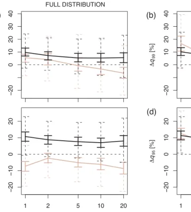
The relative quantile changes∆qfor the North Rhine region’s summer and winter are presented in Fig. 6 as a function of accumulation intervalnfor both the full distribution (left panels) and the intensity distribution (right panels).

5

Looking first at q₉₉ of the full distribution, the most extreme quantile considered (Fig. 6a), we note contrasting scaling behavior for the di_fferent seasons. In summer, a non-trivial scaling with increasing accumulation interval is observed: ∆q₉₉ is positive at 5.5% for the single-day sum, but turns negative for the 5-day sum, reaching−6.5%

for 20-day sums. In the winter,_∆q₉₉is positive across the board, between 6 and 10%,

10

and there is a relatively uniform scaling across the range of multiday sums within the estimated confidence intervals for the 17-member ensemble.

Forq₉₅ and lower quantiles of the full distribution (Fig. 6c,e,g), the summer scaling turns negative for all accumulation intervals n, and by q₅₀ the dependency on accu-mulation interval is even reversed, i.e. the fractional quantile change in the 1-day sum

15

is far more negative than for the 20-day sum. The winter scaling remains relatively uniform and positive across the accumulation periods for all quantiles.

What is the cause of the difference in scaling behavior withnbetween the summer and winter in the North Rhine region? A uniform scaling, as we see in winter, can be expected if the distributions of wet-day frequency and wet-period duration remain the

20

same while the intensity of rain days changes. Indeed, the winter intensity distribution (Fig. 6b) shows the same magnitude of uniform scaling forq₉₉ as the full distribution (Fig. 6a), indicating that the relative change must be due almost entirely to an increase in event intensity, whilst the wet-day frequency remains largely unchanged. Note that the intensity distribution atn₌1 is independent of the wet-day frequency and therefore

25

(10)

HESSD

7, 9043–9066, 2010

S. F. Kew et al.

Title Page

Tables Figures

◭ ◮

Back Close

Full Screen / Esc

Discussion

P

a

per

|

Dis

cussion

P

a

per

|

Discussion

P

a

per

|

Discussio

n

P

a

per

|

In summer, the North Rhine’s non-trivial scaling is caused by a combination of in-creased extreme intensities and reduced wet-day frequencies. Two aspects of the full distribution’s scaling behavior would be present with a reduced wet-day frequency alone: (i) the 1-day sum’s lowest quantiles decrease, leaving high quantiles hardly a_ffected – simply a consequence of raised probabilities at the ‘dry’ end of the PDF

5

(compare the magnitude of the di_fference between left hand and right hand panels of Fig. 6 for high and low quantiles at n₌1), and (ii) ∆q converges towards the mean precipitation change as the summation interval lengthens. Together, (i) and (ii) lead to the positiven-dependence of_∆q seen for low quantiles.

The added impact of increased intensities of extremes is to create a non-trivial

scal-10

ing e_ffect, whereby _∆q is positive for 1-day extremes but negative for multiday ex-tremes. The 1-day intensity distribution (Fig. 6b) shows there is a stronger positive scaling of 16.7% compared to 5.5% for the full distribution. The increase in intensity is large enough to hold_∆q₉₉ for the full distribution positive for small n, o_ff-setting the negative contribution from a reduced wet-day frequency.

15

The composition of 20-day summer extremes in both the control and future periods is such that around 80% of the sums satisfying theq₉₉ threshold contain at least one day satisfying the respective q₉₉ thresholds for single-day extremes (not shown). In other words, in many cases, it is the same event that makes a 1-day sum and 20-day sum extreme, and not persistence of moderate rainfall alone. An increase of dry/drier

20

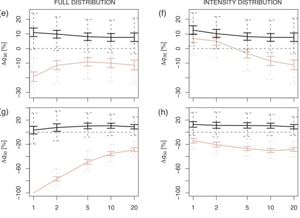
days mixed into the 20-day sum in between the extreme(s) must be the reason for the future decrease in multiday extremes. The PDF of summer wet and dry spell durations supports this showing that dry spells are projected to become longer and wet spells shorter (Fig. 6a–b).

Differences are seen between the three regions of the basin (Figs. A3, A4,

Supple-25

(11)

HESSD

7, 9043–9066, 2010

S. F. Kew et al.

Title Page

Tables Figures

◭ ◮

Back Close

Full Screen / Esc

Discussion

P

a

per

|

Dis

cussion

P

a

per

|

Discussion

P

a

per

|

Discussio

n

P

a

per

|

It is also of interest to inspect the transient simulated evolution in the seasonal cycle of monthly mean wet-day frequency and intensity (see Fig. 6 for the North Rhine and the Supplement for the other regions). It is clear to see that in summer, the change in wet-day frequency is the dominating factor, whereas in winter it is a change in intensity that will modulate the quantile changes. For the Central and Alpine regions, a decrease

5

in JJA mean intensity and wet-day frequency takes e_ffect, consistent with the more negative∆q₉₉ towards the south. These negative trends undergo acceleration during the second half of the ESSENCE simulation (see insets to figures in the Supplement). Further, it is projected that the seasonal cycles change form. In Fig. 6a, for example, it appears that for early years, the wet-day frequency follows a plateau from May to

10

September, yet at the end of the simulation, the number of wet days continues to decrease until August. The cause of this non-linearity still needs to be investigated but we expect it can be attributed to feedbacks from an extended period of drying out of the soil.

5.2 Sensitivity to ensemble size

15

The non-trivial scaling seen for the North Rhine region in summer was detected us-ing a 17 member ensemble. Current discharge estimates are based on much smaller datasets providing between 30 and 90 years of integration for each timeslice (equiva-lent to 1–3 ensemble members here). In this section we simulate smaller ensembles using the bootstrap method to see if they are also capable of reproducing the non-trivial

20

scaling and a climate signal that is significantly di_fferent from zero.

For the North Rhine region, Fig. 6 shows the 63% and 95% confidence intervals of

∆q₉₉ for 1-day and 20-day sums estimated from 10000 samples for each ensemble size, in summer and winter. In summer, Fig. 6a, around 240 years (8 members) are needed to detect the _∆q₉₉ signal as significantly di_fferent from zero. The di_fferent

25

(12)

HESSD

7, 9043–9066, 2010

S. F. Kew et al.

Title Page

Tables Figures

◭ ◮

Back Close

Full Screen / Esc

Discussion

P

a

per

|

Dis

cussion

P

a

per

|

Discussion

P

a

per

|

Discussio

n

P

a

per

|

20-day∆q₉₉signal for each of the bootstrapped samples used in Fig. 6a for ensembles of sizes 1 and 3. The peak in the density of scattered points lies in the lower right hand quadrant, where _∆q₉₉ for the 1-day sum is positive and _∆q₉₉ for the 20-day sum is negative. However, a small fraction of points lie in the opposite quadrant, showing that, for small ensembles, even the opposite scaling behavior withncan be attained.

5

In winter, Fig. 6b, for the 17-member ensemble, there is a small di_fference in scaling behavior between 1 and 20-day extremes but this difference is not significant and is not distinguishable for smaller ensembles (Fig. 6b). The 1-day scaling is significantly di_fferent from zero for an ensemble with 2 or more members, whereas the 20-day scaling requires 9 members for the same level of confidence.

10

Note the large range including both positive and negative values of_∆q₉₉ that might be obtained if just 30 years of integration (1 member) or even 90 years (3 members) are used. Confidence interval estimates of ∆q using 10 000 1-member simulations are also added (dashed error bars) to Fig. 6. They illustrate the magnitude of uncer-tainty associated with 30 years input of large scale boundary conditions to hydrological

15

models.

The size of ensemble necessary to distinguish an externally forced signal depends on the strength of the signal as well as the magnitude of internal variability. Towards the south of the basin, smaller ensembles are sufficient to distinguish the multiday response (∆q₉₉) from zero, as the signal strengthens while internal variability is of the

20

same magnitude on the scale of the basin (Figs. A7, A8, Supplement).

6 Summary and discussion

For the first time, a GCM ensemble large enough to detect the climate signal over internal variability has been used to detect a dependence of future changes in upper quantiles of precipitation on the length of the accumulation period on the scale of the

25

(13)

HESSD

7, 9043–9066, 2010

S. F. Kew et al.

Title Page

Tables Figures

◭ ◮

Back Close

Full Screen / Esc

Discussion

P

a

per

|

Dis

cussion

P

a

per

|

Discussion

P

a

per

|

Discussio

n

P

a

per

|

The dependence of extremes on the accumulation interval is limited to the sum-mer season and is strongest in the North of the basin, where one-day sum extremes increase by around 6% and 20-day sums decrease by a similar degree. This result has implications for the delta change downscaling technique. In its simplest form, the delta change method applies a single factor multiplication (consistent with mean changes in

5

climate parameters) to transform a historical time series into a future scenario for in-put into hydrological models. Such an approach would result in a change of the same sign for both single and multiday precipitation quantiles, so would not be capable of reproducing the results here. A more complex transformation is required; certainly one which first takes the change in wet-day frequency into account (e.g. Van den Hurk

10

et al., 2007), and at best in a highly controlled manner (akin to some bias correction methods, e.g. Te Linde et al., 2010). The quantile scaling technique (Shabalova et al., 2003; Leander and Buishand, 2006) using an exponential in place of linear transforma-tion to adjust the intensity of the remaining wet-day amounts can be used to achieve a more appropriate future variance. Even with these adjustments, there is no guarantee

15

that the constructed future time series will include an appropriate, uncertainty-spanning range of changes in the sequences of events, e.g. long dry periods followed by intense rain. These can only be captured and assessed by a realistic handling/modeling of the changes in large-scale circulation regimes and surface-atmosphere feedbacks.

On the other hand, in winter, relative changes of the quantiles are positive and are

20

modulated mainly by increased intensities. The simple delta change technique could be adequate for modeling basin-scale changes to the winter precipitation. Ensemble mean wet-day frequencies and the distribution of wet and dry period durations remain basically unchanged. Thus for the model and emission scenario used here, any circula-tion change that does occur does not impact the wet event frequency or duracircula-tion much,

25

although within individual transient realisations, circulation and precipitation extremes may be linked within the natural climate variability.

(14)

HESSD

7, 9043–9066, 2010

S. F. Kew et al.

Title Page

Tables Figures

◭ ◮

Back Close

Full Screen / Esc

Discussion

P

a

per

|

Dis

cussion

P

a

per

|

Discussion

P

a

per

|

Discussio

n

P

a

per

|

the model and scenario used, on the order of 8 ensemble members (240 years of integration per time slice) or more were needed to distinguish the climate change sig-nal in extremes of multiday precipitation sums from natural climate variations and their dependence on accumulation period. Although the coarse resolution of the GCM is a limitation, much of the results from nested RCMs are determined by their GCM

5

boundaries. Our results suggest that current discharge estimates based on dynam-ically downscaled short GCM integrations will be subject to inadequate sampling of large-scale variability.

Supplementary material related to this article is available online at:

http://www.hydrol-earth-syst-sci-discuss.net/7/9043/2010/hessd-7-9043-2010-supplement.pdf.

10

Acknowledgements. Thanks to Boris Orlowsky for helpful comments.

References

Brandefelt, J. and K ¨ornich, H.: Northern Hemisphere Stationary Waves in Future Climate Pro-jections, J. Climate, 21, 6341–6353, 2008. 9045

Christensen, J. H., Hewitson, B., Busuioc, A., Chen, A., Gao, A., Held, I., Jones, R., Kolli, R.

15

K., Kwon, W.-T., Laprise, R., Maga ña Rueda, V., Mearns, L., Men éndez, C. G., R äis änen, J., Rinke, A., Sarr, A., and Whetton, P.: Regional Climate Projections, in: Climate Change 2007: The Physical Science Basis, Contribution of Working Group I to the Fourth Assessment Report of the Intergovernmental Panel on Climate Change, edited by: Solomon, S., Qin, D., Manning, M., Chen, Z., Marquis, M., Averyt, K. B., Tignor, M. and Miller, H. L., Cambridge

20

University Press, Cambridge, UK and New York, NY, USA, 2007. 9046

Dankers, R., Christensen, O. B., Feyen, L., Kalas, M., and de Roo, A.: Evaluation of very high-resolution climate model data for simulating flood hazards in the Upper Danube Basin, J. Hydrol., 347, 319–331, 2007. 9044

Frei, C., Davies, H. C., Gurtz, J., and Sch ¨ar, C.:, Climate dynamics and extreme precipitation

25

(15)

HESSD

7, 9043–9066, 2010

S. F. Kew et al.

Title Page

Tables Figures

◭ ◮

Back Close

Full Screen / Esc

Discussion

P

a

per

|

Dis

cussion

P

a

per

|

Discussion

P

a

per

|

Discussio

n

P

a

per

|

Gillett, N., Graf, H., and Osborn, T.: Climatic change and the North Atlantic Oscillation, Geo-physical Monograph, 134, 193–209, doi:10.1029/134GM09, 2003. 9045

Hu, Z. and Wu, Z.: The intensification and shift of the annual North Atlantic Oscillation in a global warming scenario simulation, Tellus A, 56, 112–124, 2004. 9045

Hurkmans, R., Terink, W., Uijlenhoet, R., Torfs, P., Jacob, D., and Troch, P. A.: Changes in

5

streamflow dynamics in the Rhine basin under three high-resolution regional climate scenar-ios, J. Climate, 23, 679–698, 2010. 9046

Kay, A. L., Jones, R. G., and Reynard, N. S.: RCM rainfall for UK flood frequency estimation, II. Climate change results, J. Hydrol., 318, 163–172, 2006. 9044

Leander, R. and Buishand, T. A.: Resampling of regional climate model output for the simulation

10

of extreme river flows, J. Hydrol., 332, 487–496, 2006. 9055

Lenderink, G., Buishand, A., and van Deursen, W.: Estimates of future discharges of the river Rhine using two scenario methodologies: direct versus delta approach, Hydrol. Earth Syst. Sci., 11, 1145–1159, doi:10.5194/hess-11-1145-2007, 2007. 9044, 9045

Lenderink, G., van Meijgaard, E., and Selten, F. M.: Intense coastal rainfall in the Netherlands

15

in response to high sea surface temperatures: analysis of the event of August 2006 from the perspective of a changing climate, Clim. Dynam., 32, 19–33, 2009. 9045

Meehl, G. A., Covey, C., Delworth, T., Latif, M., McAvaney, B., Mitchell, J. F. B., Stouffer, R.

J., and Taylor, K. E.: The WCRP CMIP3 multi-model dataset: A new era in climate change research, B. Am. Meteorol. Soc., 88, 1383–1394, 2007. 9045

20

Naki´cenovi´c, N., Alcamo, J., Davis, G., de Vries, B., Fenhann, J., Gaffin, S., Gregory, K.,

Grubler, A., Jung, T. Y., Kram, T., La Rovere, E. L., Michaelis, L., Mori, S., Morita, T., Pepper, W., Pitcher, H. M., Price, L., Riahi, K., Roehrl, A., Rogner, H.-H., Sankovski, A., Schlesinger, M., Shukla, P., Smith, S. J., Swart, R., van Rooijen, S., Victor, N., and Dadi, Z.: Special Report on Emissions Scenarios: A Special Report of Working Group III of the

Intergovern-25

mental Panel on Climate Change, Cambridge University Press, Cambridge, UK, 599 pp., 2000. 9046

Pinto, J. G., Ulbrich, U., Leckebusch, G. S., Spangehl, T., Reyers, M., and Zacharias, S.: Changes in storm track and cyclone activity in three SRES ensemble experiments with the ECHAM5/MPI-OM1 GCM, Clim. Dynam., 29, 195–210, 2007. 9045

30

(16)

HESSD

7, 9043–9066, 2010

S. F. Kew et al.

Title Page

Tables Figures

◭ ◮

Back Close

Full Screen / Esc

Discussion

P

a

per

|

Dis

cussion

P

a

per

|

Discussion

P

a

per

|

Discussio

n

P

a

per

|

Shabalova, M. V., van Deursen, W. P. A., and Buishand, T. A.: Assessing future discharge of the river Rhine using regional climate model integrations and a hydrological model, Clim. Res., 23, 233–246, 2003. 9044, 9055

Sprokkereef, E.: A hydrological database for the Rhine basin (in German)/Eine hydrologische datenbank f ¨ur das Rheingebiet, Technical report, Int. Comm. for the Hydrol. of the Rhine

5

Basin, Arnhem, The Netherlands, 2001. 9047

Sterl, A., Severijns, C., Dijkstra, H., Hazeleger, W., van Oldenborgh, G. J., van den Broeke, M., Burgers, G., van den Hurk, B., van Leeuwen, P. J., and van Velthoven, P.: When can we expect extremely high surface temperatures?, Geophys. Res. Lett., 35, L14703, doi:10.1029/2008GL034071, 2008. 9045, 9046

10

Te Linde, A. H., Aerts, J. C. H., Bakker A. M. R., and Kwadijk, J. C. J.: Simulating low-probability peak discharges for the Rhine basin using resampled climate modeling data, Water Resour. Res., 46, W03512, doi:10.1029/2009WR007707, 2010. 9055

Trenberth, K. E.: Conceptual framework for changes of extremes of the hydrological cycle with climate change, Climatic Change, 42, 327–339, 1999. 9045

15

Ulbrich, U. and Christoph, M.: A shift of the NAO and increasing storm track activity over Europe due to anthropogenic greenhouse gas forcing, Clim. Dynam., 15, 551–559, 1999. 9045 Van den Hurk, B., Tank, A. K., Lenderink, G., Ulden, A., van Oldenborgh, G. J., Katsman, C.,

Brink, H., Keller, F., Bessembinder, J., Burgers, G., Komen, G., Hazeleger, W., and Drijfhout, S.: New climate change scenarios for the Netherlands, Water Sci. Technol., 56, 27–33, 2007.

20

9045, 9055

Van Ulden, A. P. and van Oldenborgh, G. J.: Large-scale atmospheric circulation biases and changes in global climate model simulations and their importance for climate change in Cen-tral Europe, Atmos. Chem. Phys., 6, 863–881, doi:10.5194/acp-6-863-2006, 2006. 9045 Yin, J. H.: A consistent poleward shift of the storm tracks in simulations of 21st century climate,

25

(17)

HESSD

7, 9043–9066, 2010

S. F. Kew et al.

Title Page

Tables Figures

◭ ◮

Back Close

Full Screen / Esc

Discussion

P

a

per

|

Dis

cussion

P

a

per

|

Discussion

P

a

per

|

Discussio

n

P

a

per

|

200 km

135 km

Lobith

Fig. 1.The Rhine basin and ESSENCE grid. The basin is represented by 8 cells: 2 in the North

(18)

HESSD

7, 9043–9066, 2010

S. F. Kew et al.

Title Page Abstract Introduction Conclusions References Tables Figures ◭ ◮ ◭ ◮ Back Close

Full Screen / Esc

Printer-friendly Version Interactive Discussion Discussion P a per | Dis cussion P a per | Discussion P a per | Discussio n P a per | 0 .1 0.0 0 .2 0.4 0 .6 0.8 1 .0

Dry event frequency

JJA 1−day sum [mm]

.1 .5 5 50

0.00 0.05 0.10 0.15 0.20 we f

* probability density

0 .1 0.0 0 .2 0.4 0 .6 0.8 1 .0

Dry event frequency

.5 2 5 20 100

0.0 0 .2 0.4 0 .6 we f

0 .1 0.0 0 .2 0.4 0 .6 0.8 1 .0

Dry event frequency

1 2 5 20 50 200

0.0 0 .2 0.4 0 .6 0.8 we f

0 .1 0.0 0 .2 0.4 0 .6 0.8 1 .0

Dry event frequency

DJF 1−day sum [mm]

.1 .5 5 50

0.00

0.10

0.20

we

f

0 .1 0.0 0 .2 0.4 0 .6 0.8 1 .0

Dry event frequency

.5 2 5 20 100

0.0 0 .2 0.4 0 .6 we f

0 .1 0.0 0 .2 0.4 0 .6 0.8 1 .0

Dry event frequency

1 2 5 20 50 200

0.0 0 .2 0.4 0 .6 0.8 we f

(a)

(d) (e) (f)

(b) (c)

Fig. 2. North Rhine control period validation of ESSENCE against CHR-OBS PDFs for JJA

(top row) and DJF (lower row) for 1-, 10- and 20-day sums (left-right). The color shading envelops the 95% range of the probability density attained from individual ensemble members, dashed white shows the mean. Black dots show CHR-OBS binned observations and the black curve is a fit estimating the CHR-OBS frequency distribution. The frequency of dry events (separate column, left of each PDF) plus the integrated PDF of wet events (scaled by the wet

event frequency,wef) together sum to unity. Vertical lines mark the locations of the 50% (thick)

(19)

HESSD

7, 9043–9066, 2010

S. F. Kew et al.

Title Page

Tables Figures

◭ ◮

Back Close

Full Screen / Esc

Discussion

P

a

per

|

Dis

cussion

P

a

per

|

Discussion

P

a

per

|

Discussio

n

P

a

per

|

−20

0

10

20

30

40

FULL DISTRIBUTION

Δ

q99

[%]

−20

0

10

20

30

40

INTENSITY DISTRIBUTION

Δ

q99

[%]

−20

−

10

0

1

0

2

0

Δ

q95

[%]

−20

−

10

0

1

0

2

0

Δ

q95

[%]

(a) (b)

(c) (d)

1 2 5 10 20

Accumulation interval n [days]

1 2 5 10 20

(20)

HESSD

7, 9043–9066, 2010

S. F. Kew et al.

Title Page

Tables Figures

◭ ◮

Back Close

Full Screen / Esc

Discussion

P

a

per

|

Dis

cussion

P

a

per

|

Discussion

P

a

per

|

Discussio

n

P

a

per

|

−30

−

10

0

1

0

2

0

Δ

q90

[%]

−30

−

10

0

1

0

2

0

Δ

q90

[%]

1 2 5 10 20

−100

−60

−

20

Δ

q50

[%]

1 2 5 10 20

−100

−60

−

20

Δ

q50

[%]

(e) (f)

(g) (h)

FULL DISTRIBUTION INTENSITY DISTRIBUTION

Fig. 3. The projected changes in quantiles (top to bottom: q₉₉, q₉₅, q₉₀, q₅₀) of 1–20 day

(21)

HESSD

7, 9043–9066, 2010

S. F. Kew et al.

Title Page

Tables Figures

◭ ◮

Back Close

Full Screen / Esc

Discussion

P

a

per

|

Dis

cussion

P

a

per

|

Discussion

P

a

per

|

Discussio

n

P

a

per

|

1 2 5 10 20

0.00

0.10

0.20

0.30

JJA wet period duration [days]

Probability density

1 2 5 10 20

0.0

0.1

0.2

0.3

0

.4

JJA dry period duration [days]

Probability density

1 2 5 10 20 50

0.00

0.05

0.10

0.15

DJF wet period duration [days]

Probability density

1 2 5 10 20

0.0

0

.2

0.4

0.6

DJF dry period duration [days]

Probability density

(a)

(c) (d)

(b)

Fig. 4.Probability density functions for wet (left) and dry (right) durations in JJA (top row) and

(22)

HESSD

7, 9043–9066, 2010

S. F. Kew et al.

Title Page

Tables Figures

◭ ◮

Back Close

Full Screen / Esc

Discussion

P

a

per

|

Dis

cussion

P

a

per

|

Discussion

P

a

per

|

Discussio

n

P

a

per

|

Monthly wet day frequency

0.4

0

.5

0.6

0

.7

0.8

0

.9

1950 2100

0.45

0.60

1950 2100

0.75

0.90

−28.8%

−2.1%

Month

Monthly intensity [mm

day

−

1 ]

D J F M A M J J A S O N

3.0

3

.5

4.0

4

.5

1950 2100

3.0

3

.4

1950 2100

3.6

4

.0

−1.4%

+14.3%

(a)

(b)

Fig. 5.Projected evolution of the seasonal cycle in wet-day frequency(a)and in intensity(b)

(23)

HESSD

7, 9043–9066, 2010

S. F. Kew et al.

Title Page

Tables Figures

◭ ◮

Back Close

Full Screen / Esc

Discussion

P

a

per

|

Dis

cussion

P

a

per

|

Discussion

P

a

per

|

Discussio

n

P

a

per

|

5 10 15

−20

−

10

0

1

0

2

0

Ensemble size [members]

Δ

q99

[%]

5 10 15

−10

−

5

0

5

1

0

1

5

2

0

2

5

Ensemble size [members]

Δ

q99

[%]

(a) (b)

JJA DJF

1-day sum

20-day sum

1-day sum

20-day sum

Fig. 6.Sensitivity ofq₉₉ scaling to ensemble size for 1 day sums (gray shading, black dots)

and 20 day sums (color shading, white dots) in JJA(a)and DJF(b), North Rhine. Confidence

intervals of 63% and 95%, approximately corresponding to 1σ and 2σ standard deviations,

(24)

HESSD

7, 9043–9066, 2010

S. F. Kew et al.

Title Page

Tables Figures

◭ ◮

Back Close

Full Screen / Esc

Discussion

P

a

per

|

Dis

cussion

P

a

per

|

Discussion

P

a

per

|

Discussio

n

P

a

per

|

−40 −20 0 20 40

y=x

M=1 M=3

M=3

M=1

Δq99 [%], 1−day sum

Δ

q99

[%], 20−day sum

63

95 63

95

−40 −20 0 20 40

y=x

M=1 M=3

M=3

M=1

Δq99 [%], 1−day sum

Δ

q99

[%], 20−day sum

95

63 95

63

(a) (b)

JJA DJF

Fig. 7.Density plots for JJA(a)and DJF(b)showing the relationship between the 1-day

sum-and 20-day sum-values of∆q₉₉found in the bootstrapped samples of Fig. 6 for ensembles with

M₌1 (white points) andM₌3 (color points) members. Density contours enclosing 63% and