www.clim-past.net/12/769/2016/ doi:10.5194/cp-12-769-2016
© Author(s) 2016. CC Attribution 3.0 License.
The WAIS Divide deep ice core WD2014 chronology – Part 2:
Annual-layer counting (0–31 ka BP)
Michael Sigl1,2, Tyler J. Fudge3, Mai Winstrup3,a, Jihong Cole-Dai4, David Ferris5, Joseph R. McConnell1, Ken C. Taylor1, Kees C. Welten6, Thomas E. Woodruff7, Florian Adolphi8, Marion Bisiaux1, Edward J. Brook9, Christo Buizert9, Marc W. Caffee7,10, Nelia W. Dunbar11, Ross Edwards1,b, Lei Geng4,5,12,d, Nels Iverson11, Bess Koffman13, Lawrence Layman1, Olivia J. Maselli1, Kenneth McGwire1, Raimund Muscheler8, Kunihiko Nishiizumi6, Daniel R. Pasteris1, Rachael H. Rhodes9,c, and Todd A. Sowers14
1Desert Research Institute, Nevada System of Higher Education, Reno, NV 89512, USA
2Laboratory for Radiochemistry and Environmental Chemistry, Paul Scherrer Institute, 5232 Villigen, Switzerland 3Department of Earth and Space Sciences, University of Washington, Seattle, WA 98195, USA
4Department of Chemistry and Biochemistry, South Dakota State University, Brookings, SD 57007, USA 5Dartmouth College Department of Earth Sciences, Hanover, NH 03755, USA
6Space Science Laboratory, University of California, Berkeley, Berkeley, CA 94720, USA
7Department of Physics and Astronomy, PRIME Laboratory, Purdue University, West Lafayette, IN 47907, USA 8Department of Geology, Lund University, 223 62 Lund, Sweden
9College of Earth, Ocean, and Atmospheric Sciences, Oregon State University, Corvallis, OR 97331, USA 10Department of Earth, Atmospheric, and Planetary Sciences, Purdue University, West Lafayette, IN 47907, USA 11New Mexico Bureau of Geology & Mineral Resources Earth and Environmental Science Department,
New Mexico Tech, Socorro, NM 87801, USA
12Department of Atmospheric Sciences, University of Washington, Seattle, WA 98195, USA 13Lamont-Doherty Earth Observatory, Columbia University, Palisades, NY 10964, USA
14Department of Geosciences and Earth and Environmental Systems Institute, Pennsylvania State University,
University Park, PA 16802, USA
anow at: Centre for Ice and Climate, University of Copenhagen, Juliane Maries Vej 30, 2100 Copenhagen, Denmark bnow at: Department of Physics, Curtin University, Perth, Western Australia 6845, Australia
cnow at: Department of Earth Sciences, University of Cambridge, Cambridge, CB2 3EQ, UK
dnow at: Laboratoire de Glaciologie et Géophysique de l’Environnement (LGGE), Université Grenoble Alpes,
3800 Grenoble, France
Correspondence to:M. Sigl ([email protected])
Received: 12 June 2015 – Published in Clim. Past Discuss.: 24 July 2015
Revised: 10 February 2016 – Accepted: 25 February 2016 – Published: 30 March 2016
Abstract.We present the WD2014 chronology for the upper part (0–2850 m; 31.2 ka BP) of the West Antarctic Ice Sheet (WAIS) Divide (WD) ice core. The chronology is based on counting of annual layers observed in the chemical, dust and electrical conductivity records. These layers are caused by seasonal changes in the source, transport, and deposi-tion of aerosols. The measurements were interpreted man-ually and with the aid of two automated methods. We val-idated the chronology by comparing to two high-accuracy,
absolutely dated chronologies. For the Holocene, the cos-mogenic isotope records of 10Be from WAIS Divide and
14C for IntCal13 demonstrated that WD2014 was
the Younger Dryas–Preboreal transition (11.595 ka; 24 years younger) and the Bølling–Allerød Warming (14.621 ka; 7 years younger), WD2014 ages are within the combined uncertainties of the timescales. Given its high accuracy, WD2014 can become a reference chronology for the South-ern Hemisphere, with synchronization to other chronologies feasible using high-quality proxies of volcanism, solar ac-tivity, atmospheric mineral dust, and atmospheric methane concentrations.
1 Introduction
Polar ice cores are a powerful tool for investigating past changes in the Earth’s climate and are the only direct mea-sure of past concentration of greenhouse gases in the atmo-sphere (Monnin et al., 2001; Siegenthaler et al., 2005; Mar-cott et al., 2014). Ice cores also provide insight into other cli-mate forcing mechanisms, such as atmospheric dust loading (Lambert et al., 2008), volcanic eruptions (Sigl et al., 2014), and biomass burning (Ferretti et al., 2005). The drilling site for the West Antarctic Ice Sheet (WAIS) Divide (WD) ice core (79.48◦S, 112.11◦W; 1766 m above sea level) was se-lected to obtain a precisely dated, high time resolution ice core record that would be the Southern Hemisphere equiv-alent of the deep Greenland ice cores (Greenland Ice-Core Project Members, 1993; NGRIP-Project-Members, 2004; NEEM community members, 2013; Taylor et al., 1997). The relatively high annual snowfall rate of 22 cm ice equivalent per year and the thick ice enable the development of a long annual-layer-based timescale.
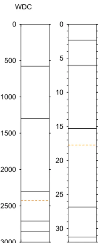
A previous chronology, WDC06A-7 (WAIS Divide Project Members, 2013), was constructed mainly by in-terpreting the seasonal variations of the electrical proper-ties of the ice and for some sections also the ice chem-istry (Fig. 1). This chronology, WD2014, supersedes that ef-fort by considering additional, seasonally varying parameters over larger sections. The WD2014 chronology is validated by comparison to the tree-ring-based IntCal13 (Reimer et al., 2013) and the U–Th-decay-based Hulu Cave chronology (Edwards et al., 2016), which are absolutely dated chronolo-gies with small uncertainties. WD2014 extends to 31.2 ka BP (thousands of years before present, with present defined as 1950 CE) and provides the WAIS Divide ice core with a timescale that has a similar resolution and accuracy to that of the deep Greenland ice cores (e.g. the layer-counted Green-land Ice Core Chronology, GICC05). For ages older than 31.2 ka, we are no longer confident that we can identify all the annual layers. Thus, below 2850 m, WD2014 is dated by stratigraphic matching of methane as described in the com-panion paper of Buizert et al. (2015).
0
500
1000
1500
2000
2500
3000
0
5
10
15
20
25
30 WDC
Figure 1.Overview of the data sets used for development of WAIS Divide annual-layer dating chronologies. Left: depth and age in-formation for the WAIS Divide aerosol records obtained at the Desert Research Institute (DRI) and South Dakota State Univer-sity (SDSU), and ECM–DEP (electrical conductivity measurement– dielectric profiling) data used to establish the new WD2014 chronology. Right: data sets used for development of the previous WDC06A-7 chronology. Also shown is the position of the acidity anomaly (17.8 ka event), a major chronostratigraphic age marker across West Antarctica (Hammer et al., 1997; Jacobel and Welch, 2005). Aerosol data below 2300 m (> 15 ka) are from insoluble par-ticle measurements (i.e. dust) only.
2 Methods
2.1 Measurements
The physical characteristics of the ice and the character of the annual layers vary with depth, which results in different data sets and methods being better suited to identify the an-nual layers at different depths. The following is a discussion of the measurement methods. The measurements relevant to this work and their corresponding effective measurement res-olution are listed in Table 1.
2.1.1 Continuous flow chemical measurements
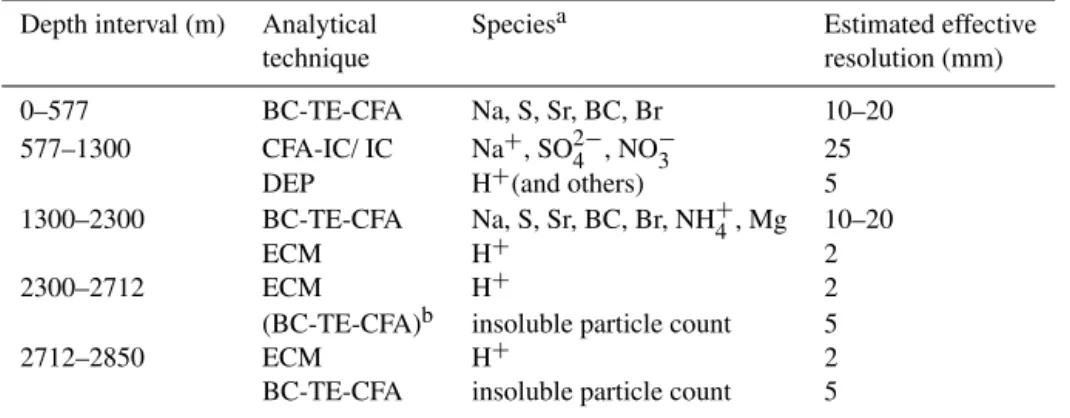
Table 1.Data used in the construction of the WD2014 ice core chronology.
Depth interval (m) Analytical Speciesa Estimated effective
technique resolution (mm)
0–577 BC-TE-CFA Na, S, Sr, BC, Br 10–20
577–1300 CFA-IC/ IC Na+, SO24−, NO−3 25
DEP H+(and others) 5
1300–2300 BC-TE-CFA Na, S, Sr, BC, Br, NH+4, Mg 10–20
ECM H+ 2
2300–2712 ECM H+ 2
(BC-TE-CFA)b insoluble particle count 5
2712–2850 ECM H+ 2
BC-TE-CFA insoluble particle count 5
aDisplayed are only species used for annual-layer dating.bThe section between 2421 and 2427 m characterized by
enhanced acid deposition (17.8 ka event) was annually layer dated using the insoluble particle count obtained from a reanalysis of a secondary longitudinal ice core section performed at the Desert Research Institute with an improved analytical set-up of the BC-TE-CFA similar to that for the ice core sections below 2712 m.
analysis (BC-TE-CFA) system (McConnell, 2002, 2010; McConnell and Edwards, 2008; McConnell et al., 2007, 2014; Pasteris et al., 2014a, b). With BC-TE-CFA analy-ses, longitudinal samples of ice core (cross-sectional area of 3.3 cm×3.3 cm and length of∼100 cm) were melted se-quentially, with the meltwater stream split into three regions. Meltwater from the innermost ring is used for inductively coupled plasma mass spectrometry (ICP-MS) using two par-allel instruments (Element 2; Thermo Scientific) and for BC mass and particle size distribution measurements using a laser-based instrument (SP2; Droplet Measurement Tech-nologies) (Schwarz et al., 2006) coupled to an ultrasonic neb-ulizer (A5000T; Cetac; Bisiaux et al., 2012; McConnell et al., 2007). Meltwater from the middle ring is used for traditional continuous flow measurements of nitrate, liquid conductiv-ity, ammonium, and pH (Pasteris et al., 2012; 2014b). Anal-yses of aerosols are complemented by addition of a laser-based particle counter (Abakus; Klotz) into the melt stream that quantifies size-resolved aerosol mass (Ruth et al., 2003). Measurements used in this study are from four analysis cam-paigns taking place between 2008 and 2014, with small ad-ditions and improvements applied to the analytical set-up over this timespan. Modifications, for example, resulted in improved resolution of the insoluble particle concentration data below 2711 m (> 28 ka) that allowed a joint annual-layer interpretation in combination with the ECM (electrical con-ductivity measurement) record. About 15 % of the core at regularly spaced intervals was rerun using duplicate samples of ice, to provide a check on issues that might adversely in-fluence the data quality over the 6-year period in which mea-surements were made.
At ice melt rates of approximately 5 cm min−1, the sys-tem achieved a depth resolution for most analytes of approx-imately 1–2 cm in ice and > 2 cm in low-density firn due to larger signal dispersion. High sampling resolution (in combi-nation with high annual snowfall rates) permits detection of
annual cycles in impurity data (Table 1; Fig. 1), a prerequisite for precise annual dating of ice core records (Rasmussen et al., 2006; Sigl et al., 2013). The BC-TE-CFA system is well suited for ice samples that are long continuous pieces. De-pending on how the instruments were configured, the annual layers had to be thicker than 2.5 cm (dust; resolution approx-imately 0.5 cm; used below 2711 m depth; see Fig. 1) or 7 cm (all other parameters) to be confidently identified.
2.1.2 Discrete chemical measurements
Between about 577 and 1300 m depth, the ice was brittle due to stress in the ice–air bubble matrix (the brittle ice zone) and the quality of the ice core was reduced. Ice core sample quality was rated poorest between 1000 and 1100 m depth, corresponding to an age interval of 4.3–4.9 ka (Souney et al., 2014). Where sample quality permitted, measurements of trace chemical impurities were performed online with a continuous flow analysis system with ion chromatography detection (CFA-IC) at the Trace Chemistry Ice Core Lab-oratory at South Dakota State University (Cole-Dai et al., 2006). This technique consists of an ice core melter linked to a group of eight ion chromatographs (four Dionex DX-600 for anion detection, four Dionex ICS-1500 for cation detec-tion). Longitudinal samples of ice core (cross-sectional area of 3.5 cm×3.5 cm) were melted sequentially at an ice melt rate of about 2.4 cm min−1, with the meltwater stream from
and analysed using traditional IC techniques (Cole-Dai et al., 2000).
2.1.3 Electrical measurements
Seasonal variations of the ice chemistry influence the electri-cal conductivity of the ice, which allow electrielectri-cal measure-ments to detect annual layering (Hammer, 1980; Taylor et al., 1997). Three types of electrical measurements were em-ployed. In the brittle ice, dielectric profiling (DEP) was used because it is insensitive to close-fitting fractures and the low spatial resolution was not a concern because the annual lay-ers were thicker than 15 cm. For the remainder of the core, two types of electrical conductivity measurements were used: alternating current (AC-ECM) and direct current (DC-ECM). The AC-ECM is primarily controlled by the acidity but also responds to other ions (Moore et al., 1992), and it can identify annual layers thicker than 2 cm. The DC-ECM is controlled by the acidity of the ice. The data quality of the DC-ECM was improved by making multiple measurements along the core, which made it possible to avoid the adverse influence of many fractures in the core. DC-ECM has the highest spa-tial resolution of all the measurements described here and can identify annual layers that are thicker than 1 cm (Taylor et al., 1997).
2.1.4 10Be measurements
10Be concentrations for the WAIS Divide ice core for
sec-tions 0–577 and 1191–2453 m depth were measured at UC Berkeley’s Space Sciences Laboratory and Purdue’s PRIME Laboratory (Woodruff et al., 2013). Sampling resolution var-ied from 1.9 to 4.2 m, but samples typically represented con-tinuous ice core sections of 3 m length. The time resolution of each sample ranged from 10 to 30 years for the past 12 kyr.
10Be/9Be ratios of all samples were measured by
accelera-tor mass spectrometry (AMS) and normalized to a10Be AMS
standard (Nishiizumi et al., 2007).10Be concentrations in the
ice and the14C content in tree rings are both influenced by
the varying flux of cosmic rays; hence,10Be measurements provide a link between the ice core and tree-ring chronolo-gies (Muscheler et al., 2014).
2.2 Seasonality in aerosol deposition
Most of the aerosol records from WAIS Divide show strong seasonal variations due to seasonality in aerosol source strength and transport efficiency, and these seasonal signals can be used to detect annual layers (Banta et al., 2008; Sigl et al., 2013). For example, Southern Hemisphere forest and grass fires usually peak during a confined burning season fol-lowing the meteorological dry period driven by seasonal in-solation changes (Bowman et al., 2009; Schultz et al., 2008; van der Werf et al., 2010), and aerosols emitted by these fires (e.g. black carbon) get transported and deposited on the
3 6 9 12 15 18 21 24
Month (Jan: 1)
14 15 16 17 18
-1
ng g
ACR Holocene
3 6 9 12 15 18 21 24
3.3 3.5 3.7 3.9 4.1
S
ACR Holocene
3 6 9 12 15 18 21 24
Month (Jan: 1)
8 12 16 20 24 28 32
-1
ng g
ACR Holocene
3 6 9 12 15 18 21 24
0.08 0.12 0.16 0.20 0.24 0.28
-1
ng g
ACR Holocene
Black
carbon
ECM
Na Nss-S
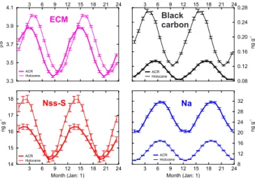
Figure 2.Average annual cycle computed for WAIS Divide ECM
record and aerosol records of Na, nssS, and BC for a 1000-year period centred over the early Holocene (10–11 ka; thin line) and Antarctic Cold Reversal (ACR; 13–14 ka; bold line). Shown are average monthly values for two complete annual cycles assuming constant snowfall distribution throughout the year. The month 0 is equivalent to the position of our annual-layer boundaries (nominal January first), broadly consistent with the minimum in [Na]. Un-certainty bars are 1σ standard error of the mean. Average WAIS Divide annual-layer thickness for the investigated time intervals is 10.0±1.6 cm a−1(Holocene) and 9.2±1.4 cm a−1(ACR).
Antarctic ice sheet (Bisiaux et al., 2012) with peak concen-trations in austral autumn.
A typical annual layer at WAIS Divide is characterized by a concentration maximum of biomass burning tracers (e.g. BC, NH+4) in austral autumn, a maximum of sea-salt depo-sition (e.g. Na, Cl) during austral winter, and a maximum of marine biogenic aerosol emission tracers (e.g. S, Br) in late austral summer (Fig. 2). Dominant sources, absolute con-centrations, and relative timing of deposition of the various aerosols are, however, not stationary through time (Fischer et al., 2007; Wolff et al., 2010). Concentrations and fluxes of Ca, Mg, and insoluble particles, for example, are low dur-ing the Holocene and are dominated by a sea-salt source (indicated by co-deposited Na and Cl), whereas during the Antarctic Cold Reversal (ACR; Fig. 2) and during the glacial (Fig. 3) concentrations and fluxes at WAIS Divide are of-ten higher by 1 order of magnitude and dominated by conti-nental dust sources (as indicated by co-deposited dust trac-ers such as V, Cr, and Ce). In contrast, BC concentrations at WAIS Divide are driven by a constant single source – natu-ral forest and savannah fires in the Southern Hemisphere – but Holocene concentrations are more than twice as large as during the late glacial period (Fig. 2).
layer-3 6 9 12 15 18 21 24
Month (Jan: 1)
6.4 6.8 7.2 7.6 8.0 8.4 8.8 -1
g dust equ. kg
DO3-DO4
3 6 9 12 15 18 21 24
3.2 3.4 3.6 3.8 4.0 4.2 S DO3-DO4
3 6 9 12 15 18 21 24
Month (Jan: 1)
40 41 42 43 44 45 -1 ng g DO3-DO4
3 6 9 12 15 18 21 24
0.118 0.122 0.126 0.130 -1 ng g DO3-DO4 ECM Black carbon Na Dust
<1.2m
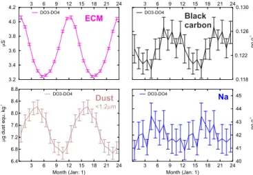
Figure 3.Average annual cycles for WAIS Divide aerosol records
similar to Fig. 2, but for a 1250-year period between the onset of Dansgaard–Oeschger (DO) events 3 and 4 (i.e. 28.1–29.4 ka), as determined from the WAIS Divide CH4record (Buizert et al., 2015). Shown are average monthly values for two complete annual cycles (January: month 1) assuming constant snowfall distribution throughout the year. Uncertainty bars are 1σ standard error of the mean. Average WAIS Divide annual-layer thickness for this interval is 3.4±0.7 cm a−1.
ing in such sections where the seasonal signal in one param-eter is overprinted by influx caused by an abnormal event.
2.3 Interpretation of individual layers
The chemical and electrical measurements discussed above contain a record of annual layers. To develop the depth–age relationship for the core, three different methods were used to identify the annual layers and thereby determine the age of the ice. Manual interpretation of the data was done by multi-ple individuals to identify the individual layers. This method is labour intensive, subjective, and can be prone to both short-term and long-term inconsistences (Alley et al., 1997; Muscheler et al., 2014; Sigl et al., 2015). Given the flexibility of a manual approach, manual interpretation may nonethe-less be the best method for interpreting time periods with an irregular or weak expression of the seasonal cycle (see Sup-plement, Figs. S1, S2). Two computer algorithms were also used to identify the annual layers. The StratiCounter algo-rithm (downloadable from https://github.com/maiwinstrup/ StratiCounter) uses methods from hidden Markov models (HMMs) and is adapted from machine speech recognition methods (Winstrup et al., 2012; Winstrup, 2016). The sec-ond method uses selection curves (McGwire et al., 2011), followed by manual adjustments in infrequent irregular sec-tions. Both methods mimic the thought process of a human making a manual interpretation. The computer algorithms re-quire less effort and can provide a more objective interpre-tation (Sigl et al., 2015). They are, however, better suited for time periods with a consistent and clear annual signal.
Age (Yrs BP 1950) 4409 DEP ( S) 3 4 5 6 nss-SO 4 (ng/g) 20 40 60 80 Na (ng/ g) 0 20 40 60 80 Depth (m)
1015.0 1015.5 1016.0 1016.5 1017.0 1017.5 1018.0
NO 3 (ng/g) 10 20 30 40 50 nss-SO 4 /Na 0.1 1 10
4411 4414 4417 4419 4422 4424
0
Figure 4.Example of a 3 m long ice core section within the WAIS Divide brittle ice zone (approximately 4400 years BP), a section for which ice core sample quality was rated poorest (Souney et al., 2014). WD2014 annual-layer markers (triangles with grey lines) are indicated. Annual layers are identified by summer and winter trac-ers: winters are characterized by maxima in [Na+]; summers are characterized by maxima in [NO−3], [nss-SO24−] and corresponding DEP maxima. Also shown is the ratio of [nss-SO24−]/[Na+].
The computer algorithms are less subjective than the manual method, but when the layering becomes difficult to interpret (e.g. during the ACR), the algorithms have to be adjusted to produce acceptable results, and these adjustments are also subjective.
The StratiCounter algorithm uses its inferred layering to optimize the layer description as function of depth, resulting in relatively few adjustable parameters. The two main inputs to the StratiCounter runs were (a) a selection of depth inter-val for initializing the algorithm based on a preliminary set of manual layer counts, thus providing the general pattern of seasonal influx of the various chemical species, and (b) a decision on whether the percentage-wise variability of layer thicknesses should be allowed to change freely with depth. The algorithm was initialized using representative sections for the different climate periods (Supplement Table S1). For the upper part, the data contained sufficient information for the algorithm to perform well when self-selecting all parame-ters used for modelling the layer shapes. For the deepest part (2711–2800 m), however, it was necessary to prescribe the percentage-wise variability of individual layer thicknesses.
constant through time and therefore not exactly the same be-tween the different subsections (Figs. 2–3).
The methods used to identify the annual layers changed with depth because the characteristics of the annual sig-nal changed with time, the quality of the ice changed with depth, and the annual-layer thickness decreased with depth due to ice flow. However, in contrast to the Greenland deep cores, most of these changes took place relatively slowly with depth, which facilitated consistent layer counting. The fol-lowing is a description of the interpretation methods used in different depth intervals.
2.3.1 Section 0–577 m (0–2345 yr BP)
In this section the high quality of the ice and thick annual layers (> 15 cm) favoured the use of the DRI continuous flow measurements. The previous WDC06A-7 timescale was sus-pected of being in error by 7 years for ages older than 700 CE because of a consistent delay of tree-ring-based surface tem-perature cooling events with respect to ice-core-based vol-canic forcing (Baillie, 2008, 2010; Baillie and McAneney, 2015). We revised the dating of the upper 577 m of the WAIS Divide core by applying the StratiCounter algorithm (Win-strup et al., 2012) using six records of Na, nssS, nssS/Na, Sr, BC, and Br. The algorithm was used between 188 m (cor-responding to the depth of the Samalas 1257 CE volcanic ice core sulfur signal) and 577 m depth. The layer-detection al-gorithm used all six parameters in parallel for the layer in-terpretation and thus produced a multi-parameter timescale based on these (Sigl et al., 2015). The annual layers were generally very clear, allowing the algorithm to be run au-tonomously and without any added constraint; manual rein-terpretation of the layer counts was not required.
2.3.2 Section 577–1300 m (2345–6009 yr BP; brittle ice zone)
For the brittle ice, where drilling fluids may have penetrated the ice through internal cracks, it is more difficult to obtain undisturbed and uncontaminated high-resolution chemistry records. The fractures precluded using the DRI continuous flow chemistry system, and measurements were instead made at South Dakota State University. Ice with many fractures was measured with discrete samples, while ice with few frac-tures was measured using continuous flow analysis (Cole-Dai et al., 2006).
Manual interpretation of annual layers was performed with non-sea-salt sulfate (nssSO24−) as the primary parameter and using Na+and NO−3 as secondary parameters (Fig. 4). When establishing WDC06A-7 (WAIS Divide Project Members, 2013), the independent DEP data set was used, with the an-nual layers initially identified with the selection curve algo-rithm (McGwire et al., 2011) subsequently manually verified or rejected. An initial reconciliation by one interpreter of the multi-parameter chemistry and DEP was performed. This
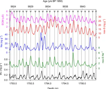
in-Figure 5.Example of a 2.5 m long ice core section of WAIS Divide (approximately 9900 years BP) with annual-layer markers (trian-gles with grey lines) indicated. Annual layers are here identified by matching pairs of winter, spring, and summer tracers. Summers are characterized by maxima in [nss-S] and corresponding ECM max-ima; autumn is indicated by maxima in [BC] from biomass burning, whereas the [Na] records show maxima in winter. Also shown is the ratio of [nss-S]/[Na].
terpretation was re-examined once the tendency for the ECM to overcount was discovered by comparison to the multi-parameter measurements (WAIS Divide Project Members, 2013) and after the comparison of10Be and14C showed the interpretation to have more years than the tree-ring timescale (see Sect. 3.1). A consensus decision was then obtained by two investigators using both data sets. The StratiCounter al-gorithm was not run for this interval because the character of the data (i.e. discrete vs. continuous measurements) is fre-quently changing. This is the first time annual layers have been identified in chemistry data through the brittle ice zone, which occurs in all deep ice cores.
Table 2.Constructing the WD2014 ice core chronology: annual-layer interpretation results using various data and interpretation techniques. N/A ice core section was not annually dated with the respective dating method or data.
Depth interval (m) 0–577 577–1300 1300–1940 1940–2020a 2020–2274 2274–2300 2300–2711 2711–2800 2800–2850
Bottom age (yr BP) 2345 6009 11 362 12 146 14 980 15 302 26 872 29 460 31 247 Mean annual-layer thicknessλ(cm) 24.0 19.7 12.0 10.2 9.0 8.1 3.6 3.4 2.8
Number
annual
layers
(rel.
to
WD2014)
Interpretation method
Consensus decision 2402 3664 5353 784 2834 322 11 570 2588 1787 I ECM Selection N/A 3704 5396 N/A 2855 322 11 567 2585 N/A
curve +40 +43 +21 0 −3 −3 (1.1 %) (0.8 %) (0.7 %) (0.0 %) (0.0 %) (−0.1 %)
II Aerosols Manual 2415 3668 5368 N/A 2843 321 N/A N/A N/A
+13 +4 +15 +9 −1
(0.5 %) (0.1 %) (0.3 %) (0.3 %) (−0.3 %)
III Aerosols StratiCounter 2402b N/A 5323 768 2645 N/A N/A 2649c N/A
0 −30 −16 −189 +61
(0 %) (−0.6 %) (−2.0 %) (−6.7 %) (+2.4 %)
aThe depth interval from 1940 to 2020 m was originally interpreted by using the combined aerosol and ECM data sets (WAIS Divide Project Members, 2013) .bThe StratiCounter algorithm was run starting from 188 m depth (1256 CE), with the uppermost part of the WDC06A-7 timescale being adopted as is.cThis section is based only on particle concentration data from the aerosol data set.
individual layer interpretations resulting from the three dif-ferent interpretation methods.
2.3.4 Section 1940–2020 m (11 362–12 146 yr BP) For this interval, a multi-parameter (aerosol and ECM) in-terpretation had already been performed for the WDC06A-7 timescale to confirm the observed sharp rise in annual-layer thickness (WAIS Divide Project Members, 2013). To esti-mate the reliability of the layer counting, the StratiCounter algorithm was also run on this interval using the multi-parameter aerosol data set (Table 2), which reconfirmed this rise in layer thicknesses. The WD2014 interpretation is un-changed from WDC06A-7 since it was based on the larger data set of both ECM and aerosol records.
2.3.5 Section 2020–2300 (12 147–15 302 yr BP)
The average annual-layer thickness during this interval was less than 10 cm (Fig. 8), making it more difficult to con-fidently identify all annual layers using the DRI continu-ous aerosol data (Fig. 6). The ECM retained sufficient mea-surement resolution. Thus, the interpretation relied upon the ECM records more than at shallower depths. The Strati-Counter algorithm was only run to 2274 m depth because we noticed that the number of annual layers detected by the StratiCounter started to slowly drift away from the other two interpretations (Table 2), which we believe to be an arte-fact arising from the lower time resolution of the data below 2000 m (Fig. S2).
2.3.6 Section 2300–2711 m (15 302–26 872 yr BP) In this depth interval, the aerosol records did not have suf-ficient depth resolution for reliable identification of the an-nual signal so the anan-nual-layer interpretation is based solely
Figure 6.Example of a 2 m long ice core section of WAIS Divide
(approximately 14 700 years BP) with annual-layer markers (trian-gles with grey lines) indicated. Similar to Fig. 5, annual layers are identified by matching pairs of winter, spring, and summer tracers. [Na] and [nss-S], determined by inductively coupled plasma mass spectrometry (ICPMS), do not always show clear annual cycles in this section with an average layer thickness of 8 cm a−1, thus
lim-iting their use for annual-layer dating in the deeper part of WAIS Divide. Annual layers are identified here using the autumn maxima in [BC] and the summer maxima in the ECM record.
bias identified during the Holocene is not directly applicable to the full length of the ice core due to the different char-acter of the annual signal in ice from the glacial and glacial– interglacial transition. Although atmospheric dust burden and deposition flux over Antarctica were higher in the glacial than in the Holocene (Fischer et al., 2007), with short-term dust deposition events noticed to occasionally obscure the ECM signals (Fig. S2), we, however, note that the compara-ble small dust input does not significantly change the shape or seasonality of the ECM signal driven by acidity input. This is best visualized in the opposing maxima of the ECM (aus-tral summer maximum) and dust (aus(aus-tral winter maximum) mean annual cycles during the Glacial (Fig. 3).
The only period of reinterpretation is for 2421.75 and 2427.25 m depth, corresponding to a period of enhanced acid deposition at WAIS Divide that forms a distinctive horizon and prominent radar reflector across West Antarc-tica (Hammer et al., 1997; Jacobel and Welch, 2005). Dur-ing this approximately 200-year-long deposition event, the annual-layer dating was based on dust particle concentra-tions. The additional measurements were made using a sec-ond stick from the main core and a modified analytical set-up with increased measurement resolution of the Abakus parti-cle counter. Annual layers in the dust were identified using the automated interpretation from the selection curve algo-rithm (McGwire et al., 2011) with manual adjustments that included the ECM data during periods without volcanic acid deposition.
2.3.7 Section 2711–2800 m (26 872–29 460 yr BP) In this section of the core, the DRI continuous analytical sys-tem was modified to increase the resolution of the particle counter measurements. This allowed insoluble particle con-centration data to also be used as an indicator of annual layers between 2711 and 2800 m depth. These data were interpreted with the StratiCounter algorithm and compared to the inter-pretation of the ECM based on the selection curve algorithm. The final timescale was mostly found by adopting the pre-vious interpretation of the ECM data, but the particle record with the StratiCounter layer interpretation was used to make manual adjustments when the ECM layer signal was ambigu-ous.
2.3.8 Section 2800–2850 m (29 460–31 247 yr BP) The annual-layer interpretation was extended using the ECM data past the 2800 m stopping depth of WDC06A-7. Parti-cle concentration data were also interpreted with the Strati-Counter algorithm, but the results were deemed unreliable with too few layers being identified, likely due to too low res-olution of the record. Layer interpretation in the ECM data below 2850 m became increasingly difficult. This difficulty in interpreting the annual cycles appears to be driven by a lack of amplitude in the annual cycle as well as decreasing
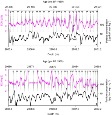
Figure 7.Example of two 0.8 m long ice core sections of WD from
(a)approximately 29 500 and (b) 29 700 years BP, with
annual-layer markers indicated. Annual annual-layers are here identified by match-ing pairs of winter and summer tracers. Summers are characterized by ECM maxima. Winters are indicated by maxima in dust depo-sition derived from the WD insoluble particle concentration record using the particle size range < 1.2 µm typical for dust transported over large distances. Dust concentrations are shown on a logarith-mic scale. Also shown is an example (2801 m) of how dust input can mask annual cycles in the ECM record by neutralizing acids present in the snowpack that are usually responsible for the annual cycle observed in electrical properties in the ice(a). The insoluble dust record provides confident and independent information on annual layering at WAIS Divide, also in the presence of acidity excursions caused by large volcanic eruptions as indicated by a 4-year-long period of increased acidity content centred at 2806.6 m depth(b).
layer thickness below 2850 m. Although an annual-layer sig-nal appears to be present in the ECM data in much of the interval from 2850 to 3100 m, we were not confident that all annual layers could be identified and we therefore terminated the annual-layer interpretation (see Fig. S3).
Depth WAIS-D (m)
0 500 1000 1500 2000 2500
A
nn
ua
l l
ay
er
th
ic
kn
es
s
(c
m
)
0 5 10 15 20 25 30 35 40
A
ge
W
D2014
(y
rs
B
P
19
50)
0 5 10 15 20 25 30 35 40
101-yr) Age WD2014
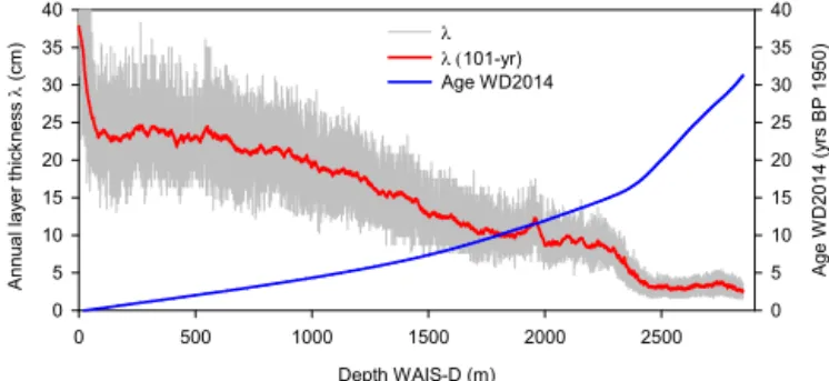
Figure 8.Depth–age profile for WAIS Divide and evolution of the annual-layer thickness (λ) for the annual-layer-dated part of the WD2014 chronology.
changes in layer thickness over this period with large transi-tions in the climate system, the decrease in layer thicknesses around 14.7 ka still takes place very gradually.
2.4 Timescale uncertainty
When establishing ice core chronologies by annual-layer in-terpretation, various sources contribute to uncertainty in the resulting timescale (see discussion in Andersen et al., 2006; Rasmussen et al., 2006). Uncertainty can be assigned to two primary causes. First, uncertainty associated with the ability of the ice core records to preserve the seasonal variations as annual layers. Second, uncertainty associated with correctly interpreting the annual layers preserved in the records.
The uncertainty associated with ability of the ice core records to preserve the annual signal occurs for several rea-sons. The primary concern is a season with abnormal weather (e.g. an exceptionally mild winter or short summer) that pre-vents the robust recording of the seasonal variations. Gaps in the data records due to low ice core quality or failure of the measurement process are negligible and have been min-imized by the use of independent measurements and data sets. During multiyear volcanic eruptions the seasonal sig-nal in some chemical and electrical records is compromised, but the black carbon recorded the annual signal because it is only influenced by biomass burning on a hemispheric scale.
The uncertainty associated with the ability to correctly in-terpret the annual layers occurs because a small percentage of the features in the records can be interpreted in several ways. To overcome this we used records indicative of multiple as-pects of the climate system (dust, black carbon from biomass burning, nssS–Na, electrical conductivity), and we used mul-tiple interpretation methods (machine-assisted interpretation and multiple manual interpreters). The vast majority of an-nual layers was clearly visible in at least one data set, but in some cases multiple interpretations were possible.
It is not possible to rigorously calculate the uncertainty of the depth–age relationship for the WAIS Divide core. Al-though there are multiple parameters that express the annual signal, and multiple methods to interpret the annual signal,
they all rely on an ice sample from the same 12 cm diame-ter cylinder from the ice sheet. We have higher confidence in depth intervals where all layer interpretations were consistent and layers appeared well resolved by the measurements. We have lower confidence deeper in the core where ice flow has thinned the layers to such extent that they are approaching the ability of the measurements to resolve them. For example, in the upper part of the ice core, all aerosol records showed clear peaks and troughs between neighbouring maxima (Figs. 4, 5, S2); in the lower part of the core, layer boundaries in some aerosol records (e.g. nssS, Na) were occasionally only recog-nizable by small inflections in the concentration data (Figs. 6 and S2).
For the GICC05 timescale, ambiguous layers were identi-fied and used to estimate uncertainty in the annual-layer in-terpretation. Each “uncertain” annual layer was counted as 0.5±0.5 years, and the half-year uncertainties were summed to determine a “maximum counting error” estimated to repre-sent a 2σ age uncertainty (Andersen et al., 2006; Rasmussen et al., 2006; Svensson et al., 2006). We did not take this ap-proach because (1) it assumes that the ice core records the seasonal variations without any bias towards recording too many or too few layers, (2) it assumes that the interpretation errors are equally split between too many and too few years, and (3) classifying the interpretation of specific individual layers as “uncertain” adds another subjective judgement to the interpretation process.
We can determine the reproducibility of the interpreta-tion by comparing manual interpretainterpreta-tions made by differ-ent people and by the machine-assisted interpretations. This approach cannot be used to rigorously determine the un-certainty of the age–depth relationship because investiga-tors conducting the interpretations influence each other when they discuss their general approach to interpreting layers, and they also determine the rules used in the machine interpreta-tions. Furthermore, this approach only considers the inter-pretation uncertainties and does not include the uncertainty associated with years that might not be recorded in the core. A comparison of different interpretations is given in Table 2. From 0 to 577 m depth, the StratiCounter-based WD2014 ages are younger than the manually derived WDC06A-7 ages by a maximum of 14 years, confirming the existence of a dating bias (Baillie and McAneney, 2015; Sigl et al., 2015) in the previous chronology. In the brittle ice section (577–1300 m), the number of annual layers derived using the multi-parameter aerosol records was 3668, which is 36 years (1 %) less than obtained using the DEP record. An ini-tial reconciliation by one interpreter of the multi-parameter and DEP records found a total of 3690 years. After re-examination, the consensus decision resulted in 3664 annual layers, which closely followed the original aerosol interpre-tation. The StratiCounter algorithm was not run on this data set.
an-nual layers were identified by the StratiCounter algorithm on the same data set, and 5396 annual layers were identified with the ECM. The consensus decision resulted in 5353 an-nual layers, slightly less (0.3 %) than the maan-nual aerosol in-terpretation, about 0.6 % more than the StratiCounter-based interpretation, and about 0.8 % less than the ECM-based in-terpretation.
For the section 1940–2020 m, the multi-parameter (aerosol and ECM) WDC06A-7 interpretation was compared with the StratiCounter interpretation based on the multi-parameter aerosol data set, which had a net difference of 16 fewer years (2 %) in the interval. From 2020 to 2274 m, the consensus de-cision found 2834 years, which was 0.3 % less than the man-ual aerosol interpretation and 0.7 % less than the ECM in-terpretation. The StratiCounter interpretation found a much smaller number of 2645 years (7 % less). At these depths, the annual-layer thickness is near the resolution limit of the aerosol measurements and thin years were not well resolved. The StratiCounter algorithm seemed to miss the small ex-pression of these layers, especially where volcanic eruptions caused disruptions of the annual-layer signal in multiple data series simultaneously. As volcanic peaks tend to obscure the annual signal in subsequent years, this may lead to some an-nual layers not being counted by StratiCounter.
Between 2200 and 2300 m depth, the total number of an-nual layers based on maan-nual interpretation from aerosols and ECM agreed within a few years. The aerosol layer interpreta-tion became increasingly difficult, and we stopped interpret-ing the multi-parameter aerosol records at 2300 m depth.
For the intervals from 2300 m to 2711 m, and between 2800 and 2850 m, where only the ECM data resolve annual layers, there is no way to test the interpretation repeatability. In sections where only ECM data were available for dating, the duration of volcanic events was dated under the assump-tion of constant annual-layer thickness, thereby resulting in less confidence in the layer interpretation.
Between 2711 and 2800 m, improved resolution of the par-ticle concentration data allowed a comparison between layer counts based on the ECM and particle concentration records. StratiCounter layer counts based on the particle concentra-tion data identified 2649 layers, which was 2 % more than the ECM-based counts.
3 Comparison to other timescales
The interpretation repeatability in Table 2 and described above is not a measurement of the accuracy of the chronology over long time periods, since over longer sections, the layer interpretation uncertainties are expected to partially cancel out assuming the absence of any consistent bias (e.g. Ras-mussen et al., 2006). To assess the accuracy of WD2014 we need to compare it to other chronologies with high ac-curacy and defined uncertainty. We have selected the tree-ring-based radiocarbon calibration chronology (Reimer et
al., 2013; Friedrich et al., 2004) and the Hulu Cave chronol-ogy (Edwards et al., 2016). The tree-ring chronolchronol-ogy was se-lected because it is considered to have virtually no age un-certainty, at least for the well-replicated time interval with high sampling coverage from present to 11.5 ka (Friedrich et al., 2004). For ages older than 25 ka, we use the Hulu Cave chronology because the radiometric dating yields small (∼100 years) age uncertainties. We describe the age com-parisons to these two records below and then assess the age accuracy for the full WD2014 timescale. We also compare WD2014 to GICC05, but since the GICC05 absolute un-certainties are large and may be underestimated during the Holocene and at the end of the glacial transition (Muscheler et al., 2014; Lohne et al., 2013, 2014), we do not use this comparison to develop estimates of the WD2014 timescale accuracy.
3.1 Comparison to tree-ring chronologies
Solar variability leads to cyclic modulation of the magnetic shielding of the Earth against galactic cosmic rays, result-ing in changes in the production rates of the cosmogenic ra-dionuclides14C and 10Be, which are both produced in the
upper atmosphere and incorporated into tree rings and ice cores, respectively. These globally synchronous variations provide a means to compare the timescales of the two proxy series by comparing ice core 10Be records with 14C pro-duction rates obtained from tree-ring14C analysis and car-bon cycle modelling (e.g. Adolphi et al., 2014; Muscheler et al., 2014). Matching cosmogenic isotope records between proxy archives has a long tradition, with numerous appli-cations existing in climate and solar sciences as well as in geochronology (Adolphi et al., 2014; Finkel and Nishiizumi, 1997; Muscheler et al., 2008; Raisbeck et al., 2007; Stein-hilber et al., 2012).
The new WD2014 timescale is consistent with indepen-dent tree-ring chronologies over the past 2400 years as demonstrated by10Be analysis obtained from WAIS Divide
(Sigl et al., 2015) for a short-lived cosmic ray anomaly de-tected in tree rings in 775 CE (Miyake et al., 2012). Further-more, ages for all major volcanic WAIS Divide sulfur sig-nals are within ±3 years of corresponding signals from a new NEEM ice core chronology over this period and from Northern Hemisphere cooling events as indicated by sum-mer temperature reconstructions from tree rings (Sigl et al., 2015). Given the constraints from historic events, the close correspondence between ages of major volcanic signals, and events observed in tree-ring data, we estimate the uncertainty envelope to be smaller than±5 years for this period.
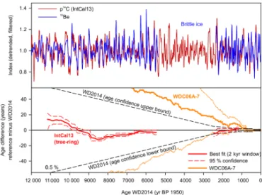
Figure 9.Comparison to the independent chronology IntCal13. Up-per panel: filtered10Be (blue) and14C (red) data on their respec-tive timescales. Lower panel: most likely time shift (red line) for the highly significant correlations together with the 2σuncertainty range inferred from ther2distribution. Results are superimposed on a WD2014 age uncertainty envelope using an absolute age un-certainty of 0.5 % over most of the Holocene. For the most recent 2500 years we estimate the uncertainty envelope to be smaller than
±5 years (Sigl et al., 2015). Also shown is the difference between the WAIS Divide chronologies (WDC06A-7 minus WD2014), indi-cating consistently younger ages for WD2014. Ice corresponding to the age interval 2.5–5.4 ka has not been sampled for10Be.
Therefore, reliable stratigraphic ties between the ice core and the tree-ring chronologies can assess the true age confidence of the WD2014 timescale.
We compare relative changes in 10Be from WAIS Divide and14C from tree rings using a Monte Carlo approach with a moving 2 kyr time window to objectively estimate the most likely time shift for synchronization (Muscheler et al., 2014). The method is described by Muscheler et al. (2014) and is summarized here. We applied filters (Muscheler et al., 2014; Vonmoos et al., 2006) to the cosmogenic isotope records to extract only variations on timescales longer than 20 years. To account for systemic carbon cycle influences on the at-mospheric14C concentration, we used a box-diffusion, car-bon cycle model (Oeschger et al., 1975; Siegenthaler, 1983) to reconstruct14C production rates (p14C) from the tree-ring measurements of atmospheric14C (Reimer et al., 2013). For
10Be, we assumed an average 1-year delay between10Be
pro-duction and deposition on the ice sheet and applied a 1-year time shift to the10Be ice core concentration data. The data were de-trended by dividing the 10Be and14C time series by their 500-year low-pass curves, thereby focusing on time periods between 20 and 500 years that show the most promi-nent longer-term solar cycles. These records were then com-pared to each other using a 2 kyr window at 100-year steps. The data are varied within the range of measurement errors (Monte Carlo approach) and within a time lag of up to+100
and−100 years between WD2014 and IntCal13. The agree-ment between the radionuclide records is determined using linear regression analysis. The time shift for the best correla-tion (maximumr2value) is considered to represent the most likely time shift (i.e. “best fit”) for synchronization. The es-timate of the uncertainty of this solution is derived from the distribution of the best fits from all iterations, since different best fits can be obtained for the different Monte Carlo real-izations (Muscheler et al., 2014). Consistent with a suggested error in the tree-ring chronology prior to 12 ka (Muscheler et al., 2014), our stepwise regression analysis does not re-trieve correlations withr2> 0.2 between WAIS Divide10Be and IntCal13 14C prior to 11.2 ka. New radiocarbon mea-surements on tree rings encompassing the Younger Dryas are currently being undertaken to further improve the calibration curve (Reimer et al., 2013; Hogg et al., 2013).
Figure 9 shows the results of the timescale comparison. The upper panel shows de-trended and normalized records for the ice core and tree-ring cosmogenic isotopes for the past 12 kyr. The lower panel gives the age difference of the timescales (IntCal13 minus WD2014) for the inferred “best fit” and 95 % confidence interval derived from the Monte Carlo approach. The close agreement at 6 ka is expected be-cause the brittle ice section of WD2014 was re-evaluated after an offset of a couple of decades to the tree-ring data was observed following the initial reconciliation. However, it should be noted that the final WD2014 age at 6 ka differs only by 4 years from the original manual interpretation of the multi-parameter aerosol records (Table 2). The maximum timescale offset is observed at approximately 8 to 9 ka when ice core ages appear to be relatively older by about 15 years. At 11 ka, WD2014 ice core ages are younger than IntCal13 by approximately 10 years (Table 3).
3.2 Comparison to a speleothem chronology
Similar to the cosmogenic radionuclides produced in the at-mosphere, methane also has a global signal and can be used to synchronize ice core records between both hemispheres (Blunier and Brook, 2001; Blunier et al., 2007) and to as-sess differences in respective age models. Further, East Asian monsoon regions – a major source area of global methane emissions – are tightly linked to rapid temperature variability in the North Atlantic region (Wang et al., 2001, 2005; Pausata et al., 2011). Rapid changes at Dansgaard–Oeschger (DO) events are distinct in both Greenland oxygen isotopes and methane and in the oxygen isotope records of stalagmites that are a proxy for the strength of the East Asian monsoon. The changes in these three parameters are expected to be near-synchronous (Buizert et al., 2015; Rosen et al., 2014; Svens-son et al., 2006, 2008), with this assumption based amongst other things on the strong coherency of their time series in the high-frequency domain (see Supplement).
Table 3.Comparison of the WD2014 ice core chronology to independent chronologies, Hulu Cave (Wang et al., 2001; Buizert et al., 2015; Edwards et al., 2016) and tree-ring-based IntCal13 radiocarbon curve (Reimer et al., 2013). A detailed description and discussion for the WAIS Divide1age estimation and synchronization procedures between the WAIS Divide CH4record Huluδ18OCalciterecord is provided
by Buizert et al. (2015).
Climate event or Age in Comparison Age in comparison Age difference (%)
comparison point WD2014 record record (yr BP) between records
8.5 ka (WAIS Divide 8500 IntCal13 8516 16 years
offset older maximum) (0.2 %)
10.5 ka (WD offset 10 500 IntCal13 10 490 10 years
younger maximum) (0.1 %)
Onset of DO3 27 755 Hulu 27 922±95 167 years
(0.6 %)
Onset of DO4 29 011 Hulu 29 134±92 123 years
(0.4 %)
Onset of DO5.1 30 730 Hulu 30 876±255 146 years
(0.5 %)
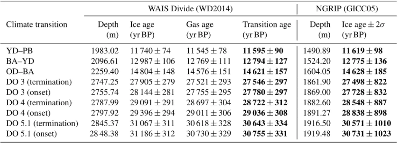
Table 4.Comparison to the independent ice core chronology GICC05 from NGRIP (Andersen et al., 2006; Rasmussen et al., 2006; Svensson et al., 2006). To calculate from WD2014 ages for rapid climate transitions (transition ages; bold) in Greenland (i.e.δ18O), we use a Greenland-CH4phasing of 50±30 years for the Younger Dryas–Preboreal (YD–PB) transition, 45±30 years for the Older Dryas to Bølling–Allerød
(OD–BA) transition and 25±30 years for all other transitions (Rosen et al., 2014; Buizert et al., 2015). A detailed description and discussion for the WAIS Divide1age estimation and synchronization procedures between the WAIS Divide CH4record and NGRIPδ18O is provided
by Buizert et al. (2015) and in the Supplement.
WAIS Divide (WD2014) NGRIP (GICC05)
Climate transition Depth Ice age Gas age Transition age Depth Ice age±2σ
(m) (yr BP) (yr BP) (yr BP) (m) (yr BP)
YD–PB 1983.02 11 740±74 11 545±78 11 595±90 1490.89 11 619±98
BA–YD 2096.61 12 987±106 12 769±111 12 794±127 1524.20 12 775±136
OD–BA 2259.40 14 804±148 14 576±151 14 621±157 1604.05 14 628±185
DO 3 (termination) 2747.25 27 905±279 27 521±293 27 546±297 1861.90 27 498±822
DO 3 (onset) 2755.74 28 144±281 27 755±295 27 780±297 1869.00 27 728±832
DO 4 (termination) 2787.99 29 091±291 28 697±304 28 722±312 1882.60 28 548±887
DO 4 (onset) 2797.92 29 396±294 29 011±306 29 036±308 1891.27 28 838±898
DO 5.1 (termination) 2845.37 31 067±311 30 618±328 30 643±334 1916.50 30 571±1010
DO 5.1 (onset) 28 48.38 31 186±312 30 730±329 30 755±331 1919.48 30 731±1023
annual-layer counted WD2014 chronology because some speleothem records, e.g. the Hulu Cave in China (Edwards et al., 2016; Wang et al., 2001), have very precise age scales (based on U–Th dating). The ice-age–gas-age differ-ence (1age) is relatively small for WD (≤525±120 years throughout the WAIS Divide core) because of the high an-nual snowfall rates at the site. The uncertainty of the lag of atmospheric CH4behind Greenlandδ18O is on the order of a
few decades (Huber et al., 2006; Baumgartner et al., 2014; Rosen et al., 2014), and the total gas-age uncertainty (for ages older than approximately 11 ka) is dominated by the cumulative annual-layer interpretation uncertainty (Table 4). The methodology and results of the methane synchronization are described in detail in the companion paper addressing the deeper part of the WD2014 chronology (see also Fig. 5 in Buizert et al., 2015).
Comparing the onset of DO 3, DO 4 and DO 5.1 as de-termined from the WD2014 gas-age scale and Hulu Cave shows that WD2014 is consistently younger than Hulu. The maximum age difference between WD2014 and Hulu is 167 years (0.6 % of the age) for the onset of DO 3 (Table 3). The WD2014 ages agree with the Hulu ages to within the com-bined Hulu age uncertainty and the WAIS Divide gas-age un-certainty (Buizert et al., 2015). The age difference between WD2014 and Hulu is much less than the cumulative uncer-tainty in identifying annual layers in WD2014.
3.3 Age accuracy
record or the Hulu Caveδ18O record. The age confidence is more difficult to determine when there are no age compar-isons. This encompasses large portions of the timescale: the brittle ice zone (2.4 ka to 5.5 ka) and the glacial–interglacial transition to the Last Glacial Maximum (LGM; 11 ka to 27 ka). Considering the interpretation repeatability (Table 2) and the comparison to the tree-ring chronology (Fig. 9), we recommend considering the ages in WD2014 to be accu-rate to better than 0.5 % in the Holocene (to 11 ka) and to have even higher precision (±5 years) during the last 2500 years. Without any comparisons for the next 16 000-year in-terval, estimating the age accuracy is difficult. The compar-isons with the Hulu Cave chronology indicate that the oldest part of the WD2014 annual timescale is accurate to within 1 % of the age, which is also supported by using an alterna-tive precisely dated cave record (Luetscher et al., 2015) from the European Alps (Fig. S4, Table S2). We suggest using a 1 % age confidence for the timescale older than 14.5 ka. Be-tween 11 and 14.5 ka, the age confidence is likely better than 1 % because there has been a limited number of years since 11 ka to accumulate uncertainty. Therefore, we linearly in-crease the age confidence from±55 years at 11 ka to±145 years at 14.5 ka.
We recognize that this is not a rigorous determination of uncertainty; however, it is the best that can be done with the information that is available now or in the foreseeable fu-ture. We assumed our errors to be random, mostly because we could avoid large systematic errors by using independent information, where possible taking advantage of the multi-ple different aerosol records (see Figs. S1, S2 for details). The assumption of random interpretation errors seems valid at least over the Holocene as demonstrated by the compara-ble small mean ice core or tree-ring age offset varying around zero (Fig. 9). We note that the uncertainty in the duration be-tween two climate events is not the difference bebe-tween the age accuracy of the two climate events. The age accuracy decreases slowly on the assumption that uncertainties in the annual-layer count will tend to cancel. Therefore, for short intervals, the uncertainty in the duration is better estimated by the interpretation repeatability, and we suggest to use 1 % during the Holocene and 2 % during the Glacial.
3.4 Comparison to the Greenland Ice Core Chronology (GICC05)
Here we summarize the observed age differences as de-rived from the methane synchronization to the GICC05δ18O chronology for rapid climate transitions within the annual-layer counted part of the WD2014 chronology (Table 4). The abrupt climate changes observed in the North Greenland Ice Core Project (NGRIP) δ18O record and leading to global methane rise (Baumgartner et al., 2014; Buizert et al., 2015) are clearly expressed during the onset of the Younger-Dryas– Holocene warming, Bølling–Allerød warming, and DO 3, DO 4, and DO 5.1, while the termination of the
interstadi-Table 5. Comparison of interval durations between WD2014,
GICC05 (NGRIP-Project-Members, 2004) and Hulu Cave (Ed-wards et al., 2016) chronologies. Years of difference are given as
reference – WD2014. We use a Greenland-CH4phasing of 50±30
years for the Younger Dryas (YD) to Preboreal (PB) transition,
45±30 years for the Older Dryas (OD) to Bølling–Allerød (BA)
transition and 25±30 years for all other transitions (Rosen et al., 2014; Buizert et al., 2015). We assume no age difference between Hulu and CH4during the transition of DO 5.1, DO 4 and DO 3.
WD2014 GICC05 Hulu
YD–PB to 1199 1156 N/A
BA–YD −43 (−4 %) N/A
BA–YD to 1827 1853 N/A
OD–BA 26 (1 %)
DO3 to 1256 1110 1212
DO4 −146 (−12 %) −44 (−4 %)
DO4 to 1720 1893 1742
DO5.1 173 (10 %) 23 (1 %)
DO3 to 2976 3003 2954
DO5.1 27 (0.9 %) −21 (−0.7 %)
N/A: not analysed
als appears more gradually (Buizert et al., 2015; NGRIP-Project-Members, 2004; Wang et al., 2001).
The absolute calendar ages for the Bølling–Allerød warm-ing and the Preboreal warmwarm-ing are slightly younger on WD2014 than GICC05 (Fig. 10) but agree within the GICC05 uncertainty. A dating correction of approximately 70 years for GICC05 for the early Holocene has recently been independently proposed based on synchronizing the Greenland Ice Core Project (GRIP)10Be record to the Int-Cal13 radiocarbon chronology (Muscheler et al., 2014) and by matching distinctive tephra horizons between Green-land ice cores and radiocarbon-dated lake sediments from Kråkenes Lake, Norway (Lohne et al., 2013, 2014). WD2014 is older than GICC05 at DO 3 by 52 years, at DO 4 by 198 years and by 24 years at DO 5.1 (Fig. 10; Table 4). The ter-minations of the DO events are all older on WD2014 than GICC05 by 49 years at DO3, 174 years at DO4, and 72 years at DO 5.1.
WDC gas age (yrs BP 1950) 31
Figure 10.Comparison between WD2014 and two independently
dated records from the Northern Hemisphere. Age differences are shown between WD2014 and GICC05 (NGRIP-Project-Members, 2004) and between WD2014 and Hulu Cave (Wang et al., 2001; Buizert et al., 2015; Edwards et al., 2016) using CH4
synchroniza-tion for time periods of rapid climate transisynchroniza-tion (i.e. NGRIPδ18O, Huluδ18Ocalcite) between 31 and 27 ka (left panel) and between
15 and 11 ka (right panel). We use a Greenland-CH4 phasing of
50±30 years for the YD–PB transition, 45±30 years for the OD– BA transition and 25±30 years for all other transitions (Rosen et al., 2014; Buizert et al., 2015). We assume no age difference
be-tween Hulu and CH4 during the transition of DO 5.1, DO 4 and
DO 3. Note the different scaling of the respectiveyaxis for the two time periods. A positive value means that the reference record is older than WD2014. Error bars represent 2σ age uncertainties of the reference chronologies. Also shown are gas-age uncertainties (black dashed line) for WD2014 (Buizert et al., 2015).
A potential concern of the WD2014 timescale is that an-nual layers might be systematically missed near the end of the timescale due to small layer thicknesses and decreasing amplitude of the seasonal cycles. To check whether this oc-curred, we compared the length of the intervals using the DO3, DO4, and DO5.1 tie points. For the entire interval from DO3 to DO 5.1, WD2014 has a very similar number of years to GICC05: 27 (1 %) fewer. The duration in the Hulu record is also quite similar, with WD2014 finding 22 (1 %) more years. This is a strong indication that WD2014 is not consistently biased and years are not being skipped. However, the difference between WD2014 and GICC05 was much greater for the two shorter intervals between DO3 and DO4 and DO4 and DO5.1: WD2014 finds 146 (13 %) more years than GICC05 in the interval between DO3 and DO4. Between DO4 and DO5.1, WD2014 finds 173 (9 %) fewer years than GICC05. These differences are large enough that they are unlikely to be fully explained by1age and matching uncertainties and likely originate, at least partially, in the un-derlying annual-layer interpretations. It is not currently pos-sible to diagnose these differences in detail. We note that the WD2014 durations differ by 4 and 1 % from the Hulu dura-tions for these shorter intervals.
4 Conclusions
WD2014 is the first multi-parameter, annual-layer-based timescale extending into the last glacial for an Antarctic ice core. This was possible due to (1) the high annual snowfall rates present at the drill site, (2) the small amount of layer thinning due to the thick ice and basal melting and (3) use of the most recent analytical techniques. The data included for the first time measurements of black carbon, a unique biomass burning tracer with strong intra-annual emission variability arising from an insolation-driven annual biomass burning cycle in the Southern Hemisphere. Annual layers were continuously identified through the brittle ice zone us-ing chemistry, which has not been done before, and with DEP. This allowed a continuous timescale to be developed without needing to match sections of multiple ice cores.
The age accuracy, as deduced by comparisons with abso-lutely dated timescales, is much better than the interpretation repeatability. The age accuracy for the Holocene (11 ka and younger) is estimated to be better than 0.5 % of the age; the age accuracy is estimated to increase to 1 % for ages older than 14.5 ka. WD2014 can become a reference chronology for Antarctic ice core records and the Southern Hemisphere equivalent of the GICC05 chronology. Synchronization be-tween ice cores can be achieved using the WAIS Divide sul-fur record of volcanic events, which does not require using the gas timescale and1age calculations, as demonstrated for the past 2000 years where 25 ice core records from Antarc-tica were synchronized to WAIS Divide (Sigl et al., 2014). Sulfate records are available for other deep ice core records from East Antarctica including Vostok (Parrenin et al., 2012), Talos Dome (Severi et al., 2012), the EPICA cores from Dronning Maud Land, and Dome C (Severi et al., 2007).
the worldwide transition from ice age climates to the present climate and their impact on ice sheets and global sea level.
The Supplement related to this article is available online at doi:10.5194/cp-12-769-2016-supplement.
Acknowledgements. This work is funded through the US
National Science Foundation grants 0839066 (to J. Cole-Dai), 1204172, 1142041, 1043518 (to E. J. Brook), 1142069, 1142115 (to N. W. Dunbar), 0839093, 1142166 (to J. R. McConnell), 1043500, 0944584 (to T. A. Sowers), 0230149, 0230396, 0440817, 0440819, 0944191, 0944348 (to K. C. Taylor), 0839042 (M. W. Caffee and T. E. Woodruff) 0839137 (to K. C. Welten) and 0944197 (supporting T. J. Fudge); the NOAA Climate and Global Change Fellowship Program, administered by the University Corporation for Atmospheric Research (to C. Buizert); and the Villum Founda-tion (to M. Winstrup). R. Muscheler and F. Adolphi are supported by the Swedish Research Council (Grant No: 2013-8421); a NASA National Earth and Space Science Fellowship also supported T. J. Fudge. The National Science Foundation Office of Polar Programs also funded the WAIS Divide Science Coordination Office at the Desert Research Institute of Nevada and University of New Hampshire for the collection and distribution of the WAIS Divide ice core and related tasks; the Ice Drilling Program Office and Ice Drilling Design and Operations group for coring activities; the National Ice Core Laboratory for curation of the core; Raytheon Polar Services for logistics support in Antarc-tica; and the 109th New York Air National Guard for airlift in Antarctica. We thank the WAIS Divide Drilling Team and science technicians who processed the ice core in the field and at the NICL. We thank Anders Svenson for performing an independent inter-pretation for parts of the ice core used to initialize the StratiCounter.
Edited by: V. Masson-Delmotte
References
Adolphi, F., Muscheler, R., Svensson, A., Aldahan, A., Possnert, G., Beer, J., Sjolte, J., Bjorck, S., Matthes, K., and Thieblemont, R.: Persistent link between solar activity and Greenland climate dur-ing the Last Glacial Maximum, Nat. Geosci., 7, 662–666, 2014. Alley, R. B., Shuman, C. A., Meese, D. A., Gow, A. J., Taylor, K. C.,
Cuffey, K. M., Fitzpatrick, J. J., Grootes, P. M., Zielinski, G. A., Ram, M., Spinelli, G., and Elder, B.: Visual-stratigraphic dating of the GISP2 ice core: Basis, reproducibility, and application, J. Geophys. Res.-Oceans, 102, 26367–26381, 1997.
Alloway, B. V., Lowe, D. J., Barrell, D. J. A., Newnham, R. M., Almond, P. C., Augustinus, P. C., Bertler, N. A. N., Carter, L., Litchfield, N. J., McGlone, M. S., Shulmeister, J., Vandergoes, M. J., Williams, P. W., and Members, N. I.: Towards a climate event stratigraphy for New Zealand over the past 30 000 years (NZ-INTIMATE project), J. Quaternary Sci., 22, 9–35, 2007. Andersen, K. K., Svensson, A., Johnsen, S. J., Rasmussen, S.
O., Bigler, M., Rothlisberger, R., Ruth, U., Siggaard-Andersen,
M. L., Steffensen, J. P., Dahl-Jensen, D., Vinther, B. M., and Clausen, H. B.: The Greenland Ice Core Chronology 2005, 15– 42 ka, Part 1: constructing the time scale, Quaternary Sci. Rev., 25, 3246–3257, 2006.
Baillie, M. G. L.: Proposed re-dating of the European ice core chronology by seven years prior to the 7th century AD, Geophys. Res. Lett., 35, L15813, doi:10.1029/2008GL034755, 2008.
Baillie, M. G. L.: Volcanoes, ice-cores and
tree-rings: one story or two?, Antiquity, 84, 202–215,
doi:10.1017/S0003598X00099877, 2010.
Baillie, M. G. L. and McAneney, J.: Tree ring effects and ice core acidities clarify the volcanic record of the first millennium, Clim. Past, 11, 105–114, doi:10.5194/cp-11-105-2015, 2015.
Banta, J. R., McConnell, J. R., Frey, M. M., Bales, R. C., and Taylor, K.: Spatial and temporal variability in snow accumulation at the West Antarctic Ice Sheet Divide over recent centuries, J. Geo-phys. Res.-Atmos., 113, D23102, doi:10.1029/2008JD010235, 2008.
Baumgartner, M., Kindler, P., Eicher, O., Floch, G., Schilt, A., Schwander, J., Spahni, R., Capron, E., Chappellaz, J., Leuen-berger, M., Fischer, H., and Stocker, T. F.: NGRIP CH4
con-centration from 120 to 10 kyr before present and its relation to aδ15N temperature reconstruction from the same ice core, Clim. Past, 10, 903–920, doi:10.5194/cp-10-903-2014, 2014.
Bisiaux, M. M., Edwards, R., McConnell, J. R., Curran, M. A. J., Van Ommen, T. D., Smith, A. M., Neumann, T. A., Pas-teris, D. R., Penner, J. E., and Taylor, K.: Changes in black car-bon deposition to Antarctica from two high-resolution ice core records, 1850–2000 AD, Atmos. Chem. Phys., 12, 4107–4115, doi:10.5194/acp-12-4107-2012, 2012.
Blockley, S. P. E., Lane, C. S., Hardiman, M., Rasmussen, S. O., Seierstad, I. K., Steffensen, J. P., Svensson, A., Lotter, A. F., Turney, C. S. M., and Bronk Ramsey, C.: Synchronisation of palaeoenvironmental records over the last 60 000 years, and an extended INTIMATE event stratigraphy to 48 000 b2k, Quater-nary Sci. Rev., 36, 2–10, 2012.
Blunier, T. and Brook, E. J.: Timing of millennial-scale climate change in Antarctica and Greenland during the last glacial pe-riod, Science, 291, 109–112, 2001.
Blunier, T., Spahni, R., Barnola, J.-M., Chappellaz, J., Loulergue, L., and Schwander, J.: Synchronization of ice core records via at-mospheric gases, Clim. Past, 3, 325–330, doi:10.5194/cp-3-325-2007, 2007.
Bowman, D. M. J. S., Balch, J. K., Artaxo, P., Bond, W. J., Carlson, J. M., Cochrane, M. A., D’Antonio, C. M., DeFries, R. S., Doyle, J. C., Harrison, S. P., Johnston, F. H., Keeley, J. E., Krawchuk, M. A., Kull, C. A., Marston, J. B., Moritz, M. A., Prentice, I. C., Roos, C. I., Scott, A. C., Swetnam, T. W., van der Werf, G. R., and Pyne, S. J.: Fire in the Earth System, Science, 324, 481–484, 2009.
Buizert, C., Cuffey, K. M., Severinghaus, J. P., Baggenstos, D., Fudge, T. J., Steig, E. J., Markle, B. R., Winstrup, M., Rhodes, R. H., Brook, E. J., Sowers, T. A., Clow, G. D., Cheng, H., Edwards, R. L., Sigl, M., McConnell, J. R., and Taylor, K. C.: The WAIS Divide deep ice core WD2014 chronology – Part 1: Methane syn-chronization (68–31 ka BP) and the gas age-ice age difference, Clim. Past, 11, 153–173, doi:10.5194/cp-11-153-2015, 2015. Cole-Dai, J., Ferris, D., Lanciki, A., Savarino, J., Baroni,