www.clim-past.net/9/2789/2013/ doi:10.5194/cp-9-2789-2013
© Author(s) 2013. CC Attribution 3.0 License.
Climate
of the Past
High-resolution mineral dust and sea ice proxy records from the
Talos Dome ice core
S. Schüpbach1,2,3, U. Federer1,2, P. R. Kaufmann1,2, S. Albani4, C. Barbante3,5, T. F. Stocker1,2, and H. Fischer1,2 1Climate and Environmental Physics, Physics Institute, University of Bern, Bern, Switzerland
2Oeschger Centre for Climate Change Research, University of Bern, Bern, Switzerland
3Environmental Sciences, Informatics and Statistics Department, University of Venice, Venice, Italy 4Department of Earth and Atmospheric Sciences, Cornell University, Ithaca, NY, USA
5Institute for the Dynamics of Environmental Processes – National Research Council, Venice, Italy
Correspondence to:S. Schüpbach ([email protected]) Received: 31 May 2013 – Published in Clim. Past Discuss.: 21 June 2013
Revised: 8 November 2013 – Accepted: 27 November 2013 – Published: 23 December 2013
Abstract.In this study we report on new non-sea salt calcium (nssCa2+, mineral dust proxy) and sea salt sodium (ssNa+, sea ice proxy) records along the East Antarctic Talos Dome deep ice core in centennial resolution reaching back 150 thousand years (ka) before present. During glacial conditions nssCa2+ fluxes in Talos Dome are strongly related to tem-perature as has been observed before in other deep Antarctic ice core records, and has been associated with synchronous changes in the main source region (southern South America) during climate variations in the last glacial. However, during warmer climate conditions Talos Dome mineral dust input is clearly elevated compared to other records mainly due to the contribution of additional local dust sources in the Ross Sea area. Based on a simple transport model, we compare nssCa2+ fluxes of different East Antarctic ice cores. From this multi-site comparison we conclude that changes in trans-port efficiency or atmospheric lifetime of dust particles do have a minor effect compared to source strength changes on the large-scale concentration changes observed in Antarctic ice cores during climate variations of the past 150 ka. Our transport model applied on ice core data is further validated by climate model data.
The availability of multiple East Antarctic nssCa2+ records also allows for a revision of a former estimate on the atmospheric CO2sensitivity to reduced dust induced iron
fer-tilisation in the Southern Ocean during the transition from the Last Glacial Maximum to the Holocene (T1). While a former estimate based on the EPICA Dome C (EDC) record only suggested 20 ppm, we find that reduced dust induced iron
fer-tilisation in the Southern Ocean may be responsible for up to 40 ppm of the total atmospheric CO2increase during T1.
During the last interglacial, ssNa+ levels of EDC and EPICA Dronning Maud Land (EDML) are only half of the Holocene levels, in line with higher temperatures during that period, indicating much reduced sea ice extent in the Atlantic as well as the Indian Ocean sector of the Southern Ocean. In contrast, Holocene ssNa+ flux in Talos Dome is about the same as during the last interglacial, indicating that there was similar ice cover present in the Ross Sea area during MIS 5.5 as during the Holocene.
1 Introduction
from Antarctic ice cores, information on accompanying re-gional environmental changes is still limited. For example, detailed information on enhanced phytoplankton productiv-ity through atmospheric dust deposition in the SO (iron fer-tilisation) (Martin, 1990) could contribute to a better under-standing of the impact of regional climate changes on the global carbon cycle. Also sea ice in the SO is a key com-ponent of the southern high latitude climate system, because an increase in its extent contributes to an increased albedo of the ocean, to a reduced gas exchange, and to decreased ocean mixing (Abram et al., 2013). Sea ice also plays a major role in the formation of deep waters in the ocean, and therefore in global ocean circulation and the carbon cycle (Toggweiler, 1999; Bouttes et al., 2010; Dieckmann and Hellmer, 2010). One possibility to assess past changes in these two param-eters are proxy-aerosol records in deep Antarctic ice cores, which provide detailed information on mineral dust deposi-tion and sea ice coverage in different regions of Antarctica (Petit et al., 1990; Röthlisberger et al., 2002; Wolff et al., 2003, 2006; Fischer et al., 2007b; Bigler et al., 2010; Abram et al., 2013).
During glacial/interglacial cycles, most of the variability in atmospheric dust concentration in central East Antarc-tica was related to the strength of remote continental mineral dust sources and to atmospheric transport efficiency (Fischer et al., 2007b; Petit and Delmonte, 2009). Southern South America (i.e. southern Patagonia) was identified to be the most important source region for glacial terrestrial aerosol transported to East Antarctica (Basile et al., 1997; Gaiero, 2007; Delmonte et al., 2008; Gabrielli et al., 2010; We-ber et al., 2012), whereas during the Holocene other remote sources become relatively more important for the dust input to East Antarctica due to the strong decline in dust mobi-lization in Patagonia (Revel-Rolland et al., 2006; Li et al., 2008; Marino et al., 2009; Gabrielli et al., 2010; Wegner et al., 2012). In addition, dust sources from ice-free areas in the periphery of Antarctica may contribute. While for high-altitude drill sites in the interior of the East Antarctic plateau (e.g. Vostok, EDC) such local sources may be insignificant, their contribution becomes more important for peripheral ar-eas (Bory et al., 2010; Delmonte et al., 2010b; Albani et al., 2012a), in particular those close to the Transantarctic Moun-tains. The TALDICE (TALos Dome Ice CorE) project pro-vides a deep ice core located at Talos Dome in the Ross Sea sector of East Antarctica in northern Victoria Land (Frezzotti et al., 2007; Stenni et al., 2011). This core is well-positioned to investigate the regional atmospheric circulation changes and their relationship with the glaciation history and envi-ronmental changes in the Ross Sea area for the past two glacial/interglacial cycles based on climate proxy as well as terrestrial and sea salt aerosol records.
Physical and chemical properties of dust analysed in Ta-los Dome snow and ice suggest that local contributions (un-consolidated glacial deposits, for example, in the Antarctic dry valleys and regolith located at high elevation in northern
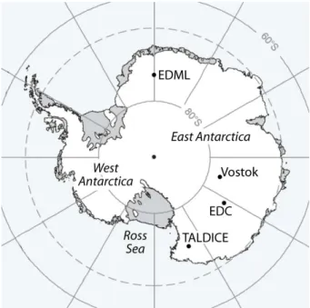
Fig. 1.Map of the Antarctic ice sheet. The four Antarctic drilling sites discussed in this work are indicated. One is located in the At-lantic sector (EDML) and, thus, closer to the southern South Amer-ican continental dust source than EDC and Vostok, both being lo-cated in the Indian Ocean sector. The fourth drilling site, TALDICE, is at a more coastal site close to the Ross Sea and, therefore also in-fluenced by local source regions especially during warm periods.
Victoria Land) to the aeolian dust input was increasing rel-ative to total dust input during the Holocene, when remote sources were low compared to the last glacial period (Del-monte et al., 2010b; Albani et al., 2012a; Del(Del-monte et al., 2013). Dust deflation and transport from proximal sources to the Talos Dome site is influenced by the availability and strength of the dust sources as well as by local meteorolog-ical conditions, which in turn are related to regional climate (Albani et al., 2012a). Despite the importance of aeolian dust transport to Antarctica, information on sources and transport of mineral dust from peripheral ice-free areas to the Antarctic interior is still limited. The spatial extent of local dust sources can be assessed by analyses of the isotopic composition of strontium (87Sr/86Sr) and neodymium (143Nd/144Nd) in the dust of the ice core samples. However, the extremely low dust concentration in ice cores during interglacial climate conditions makes such analyses extremely difficult (Petit and Delmonte, 2009; Delmonte et al., 2013).
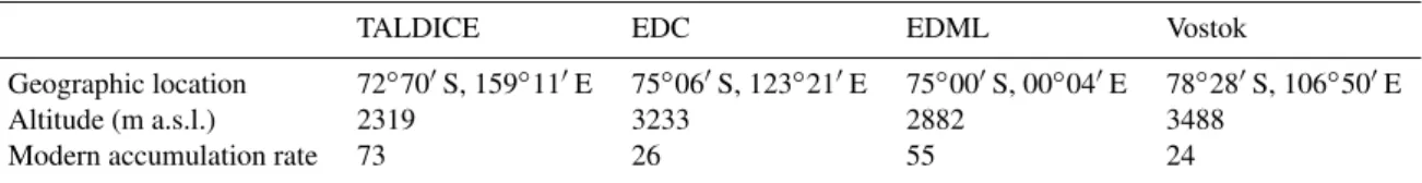
Table 1.Geographical and glaciological setting of the drill sites. Modern altitude is given in m a.s.l. (above sea level), average Holocene accumulation rates are given in (kg m−2a−1).
TALDICE EDC EDML Vostok
Geographic location 72◦70′S, 159◦11′E 75◦06′S, 123◦21′E 75◦00′S, 00◦04′E 78◦28′S, 106◦50′E
Altitude (m a.s.l.) 2319 3233 2882 3488
Modern accumulation rate 73 26 55 24
source regions for the Atlantic and Indian Ocean sector of Antarctica are spatially not the same and source strength as well as transport may have changed independently in differ-ent regions around Antarctica. Accordingly, we interpret sea salt sodium as a sea ice proxy restricted to the adjacent ocean source areas, which are the Atlantic Ocean sector of the SO for EDML, the Indian Ocean sector for EDC and Vostok, and the Ross Sea sector for TALDICE, as indicated by back tra-jectory calculations (Reijmer et al., 2002; Scarchilli et al., 2011) and by the limited atmospheric lifetime of the sea salt aerosol (Fischer et al., 2007b; Röthlisberger et al., 2010).
In this study we report on mineral dust represented by non-sea salt calcium (nssCa2+) and sea salt aerosol repre-sented by sea salt sodium (ssNa+) records from TALDICE in centennial resolution reaching back 150 thousand years be-fore present (ka BP), where present refers to 1950 AD. The new proxy data from TALDICE based on continuous flow analysis (CFA) techniques is compared to three other East Antarctic ice core records in the following, all covering at least the last 150 ka (a map of Antarctica with all investi-gated ice core sites is shown in Fig. 1; Table 1 provides fur-ther information about the sites). These are the two deep ice cores drilled within the European Project for Ice Coring in Antarctica (EPICA) at Dome C (EDC) (EPICA, 2004) and at Kohnen station in Dronning Maud Land (EDML) (EPICA, 2006), as well as the Vostok ice core (Petit et al., 1999). Fischer et al. (2007a) have already shown that a comparison of nssCa2+records of different ice cores can reveal substan-tial information about the sources and transport mechanisms of dust deposited on the East Antarctic plateau. Here we ex-tend the findings by Fischer et al. (2007a) with a multi-site comparison of nssCa2+ ice core records in centennial res-olution, complemented with model data of dust deposition on the East Antarctic plateau available for the Last Glacial Maximum (LGM) and the Holocene. In addition, the ssNa+ records of the different drill sites give indications on the evo-lution of local sea ice coverage in the Atlantic Ocean, In-dian Ocean, and Ross Sea sector of the SO during the past 150 ka BP.
2 Materials and methods
2.1 Data acquisition and performance
This study is based on high-resolution calcium (Ca2+) and sodium (Na+) CFA data from the Antarctic ice cores EDC (Röthlisberger et al., 2004; Bigler et al., 2006, 2010), EDML (Ca2+ CFA data have already been discussed in Kauf-mann et al., 2010; Na+ CFA data represent new data), and TALDICE (new data). All analyses were performed using CFA (Röthlisberger et al., 2000; Kaufmann et al., 2008), pro-viding aerosol chemistry data in unprecedented resolution and avoiding analytical blank issues, which are especially important in the case of Ca2+ (Fischer et al., 2007a; Kauf-mann et al., 2010). Besides these high-resolution data, we included Na+ and Ca2+ records from the Vostok ice core in our multi-site comparison, which are available in coarse resolution only (De Angelis et al., 1997) and are based on discrete ion chromatographic (IC) analysis of samples after manual decontamination.
CFA measurements of TALDICE were performed in the years 2006–2008 at the Alfred-Wegener-Institut (AWI) in Bremerhaven, Germany. The covered depth interval (305– 1435 m) corresponds to an age interval of 3.8–150 ka BP. Ma-jor gaps in the new TALDICE data sets can be found in the Ca2+record from 490–502 m and from 535–578 m, as well as in the Na+ record from 441–449 m, respectively. Apart from the mentioned gaps, no gaps longer than five consec-utive metres can be found in either of the new records (see Fig. 2). The longer gaps are due to maintenance and failure of the respective CFA detector, while measurements where con-tinued. Other smaller gaps are mainly due to bad ice quality (mostly in the brittle ice zone) or distinct visible (ash) layers which were not processed with CFA. Apart from these gaps, continuous records have been achieved with a sampling res-olution of 0.5 cm or better.
measurements reduces process blanks considerably com-pared to manual ice sample decontamination for IC measure-ments. As a consequence, the LOD of CFA are significantly lower compared to IC measurements.
EDML Na+ data in the age interval 123.3–132.3 ka BP (depth: 2341–2383 m) have been analysed using IC (Fischer et al., 2007a) in 1 m resolution due to missing CFA Na+data in this depth interval. On the Vostok ice core 237 discontin-uous measurements have been analysed with a mean depth resolution of 10.1 m using IC only (De Angelis et al., 1997). Each individual Vostok ice sample (once decontaminated by rinsing) was generally 10 cm long. Of these measurements, covering a depth range of 100–2500 m, we show 218 data points which represent the age range 5–150 ka BP, resulting in a mean age resolution of 665 yr.
2.2 Data treatment and dating
In order to compare the different ice cores, the different resolutions of the data sets have to be considered. There-fore, equidistant age averages (100 and 500 yr for all the high-resolution records, and 500 yr only for the Vostok records) were calculated for all four ice cores using the well-synchronised recent AICC2012 age scales (Bazin et al., 2013; Veres et al., 2013). In the following we describe how this is achieved based on the three high-resolution records and the discrete IC records of Vostok ice core.
The age scale (given in 1–3 m resolution, depending on the ice core and depth range) has been interpolated to assign an age to each individual data point of the high-resolution records. In the same way the accumulation rates have been interpolated in order to calculate deposition fluxes and to re-construct the atmospheric signals (see next section). Cen-tennial medians have then been calculated from the high-resolution data on the common age scale for each record. Medians have been calculated to prevent the hundred year mean values from being biased by single extreme events. The number of high-resolution data points per 100 yr interval ranges from 6000 (Holocene) to 77 (during the penultimate glacial, i.e. 140 ka BP) due to the increasing thinning of the ice layers towards the bottom. If more than two thirds of the high-resolution data within the interval, from which a 100 yr median has been calculated, were missing, the median has been discarded, again in order to prevent an extreme event to bias the result significantly. The same threshold has been applied for the calculation of the 500 yr medians. With this threshold we discarded up to 7 % of the calculated data of a single record.
For the Vostok records, available in coarser resolution only, we simply interpolated the age scale to assign an age to each data point at its individual depth. From these data points we then interpolated Na+and Ca2+concentrations to obtain a value for each 500 yr step in accordance with the 500 yr means of the three other cores. No 100 yr values have been calculated for Vostok due to the coarse resolution of
the original data sets. We acknowledge that this is an inaccu-rate treatment from a statistical point of view. However, the records we obtain in this way are used for illustrative purpose only, while the significance is in no way comparable to the records of the other three cores.
2.3 Crustal, sea salt, and flux correction
In addition to water-insoluble mineral dust particles, also water-soluble Ca2+ ions can be considered as a valuable ice core proxy of continental aerosol input onto the East Antarctic ice sheet. However, not only continental sources emit Ca2+ but also sea water can have a considerable con-tribution to the total Ca2+load in the air masses, especially during interglacial periods. Sodium on the other hand origi-nates mainly from the marine source, but has some continen-tal source contribution as well. Thus, the sea water contribu-tion has to be subtracted from the total Ca2+signal in order to obtain the nssCa2+concentration representing continental dust input. On the other hand, the continental contribution has to be subtracted from total Na+ in order to obtain the ssNa+signal only. In all four ice core records the nssCa2+ and the ssNa+fractions, respectively, are calculated from the Ca2+and Na+records according to Bigler et al. (2006), us-ing an empirical Antarctic ice core specific crustal correction for Ca2+and Na+, respectively.
Calcium and sodium are both conservatively deposited onto the ice sheet, thus there is no need to account for additional post-depositional effects distorting the signals in the ice.
that in contrast to EDC and Vostok, where dry deposition is predominant, EDML and Talos Dome are more interme-diate accumulation sites (see Table 1 for average Holocene accumulation rates). Thus, wet deposition can have a signifi-cant influence on the deposition fluxes, potentially introduc-ing additional variations in the calculated flux rates of EDML and TALDICE data used in this work. Furthermore, the un-certainties of the modelled accumulation rates are usually around 20 %. Together with the estimated concentration er-rors, which are below 10 %, the uncertainties of the total de-position fluxes are estimated to be smaller than 30 %. Even though this estimated error is considerable, it is small com-pared to glacial/interglacial nssCa2+flux changes, which are of the order of one magnitude.
2.4 Model for aerosol transport
In order to discuss our proxy-aerosol data and compare them with other East Antarctic ice core records, we applied a sim-ple exponential transport model which is presented in the fol-lowing. Assuming a simple model of atmospheric aerosol transport as described by Fischer et al. (2007a) with an aerosol concentrationCair(0)at the source and an
exponen-tial loss during transport, the concentration of the aerosol in the air parcel at any timet can be described as
Cair(t )=Cair(0)·exp(−t /τ ),
whereτ is the average atmospheric residence time of the aerosol. Using this simple transport model and assuming a single source region (e.g. Patagonia), the logarithmic air con-centration of the aerosol at one site (e.g. EDC) with trans-port timet2from the source location to the site can be
ex-pressed by the concentration at another site (e.g. EDML) with transport timet1according to
ln [Cair(t2)]=ln [Cair(t1)]−1t /τ,
where 1t=t2−t1 is the difference of the transport times
from the source to the two sites, assuming that the atmo-spheric residence time along the two transport ways is the same. Thus the relation of the logarithms of the atmospheric aerosol concentration at the two drilling sites is linear to first order with an offset1t /τ.
3 Results and discussion
3.1 The main features of the new TALDICE non-sea salt calcium and sea salt sodium records
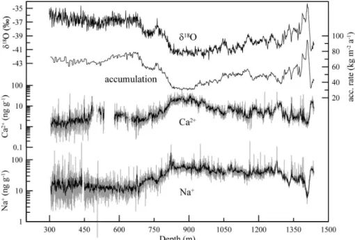
In this publication we present the first continuous high-resolution records of Ca2+and Na+of the Talos Dome ice core. The concentrations of the two species are shown in Fig. 2 versus depth in 10 cm and 1 m resolution along with the TALDICEδ18O profile in 1 m resolution (Stenni et al.,
2011) and the age scale derived accumulation rate at Ta-los Dome. Since part of the concentration changes seen in Fig. 2 are simply due to the fact that the snow accumula-tion rate is changing considerably (more than a factor of two, see 2nd panel in Fig. 2) over glacial/interglacial cycles, we will discuss the fluxes of the source separated signals in the following.
The different East Antarctic nssCa2+flux records are dis-cussed and compared in Sect. 3.3 and Sect. 3.4. While the fluxes of EDC and EDML evolved synchronously during the past 150 ka with a constant offset, the TALDICE nssCa2+ flux seems to oscillate between the other two records. Inter-estingly, TALDICE values are following the EDC flux during cold periods, while during warmer periods (grey shaded pan-els in Fig. 3) they are considerably higher than in EDC. This observation is discussed in Sect. 3.4.2, while in Sect. 3.4.1 nssCa2+ fluxes of EDC and EDML are compared in more detail. In the following section (Sect. 3.2) ssNa+flux is dis-cussed and compared with the EDC and EDML records over the past 150 ka.
3.2 Sea salt sodium
3.2.1 The last glacial period
During cold periods the sea salt flux is rather constant in all three ice cores compared to coeval ice extent changes in-ferred from marine sediment data. The sea salt flux in ice cores appears to be increasingly insensitive for very large sea ice extents as a result of the vast source area available, when the sea ice around Antarctica extends further north. Addition-ally, the distance from the sea ice margin to the drill sites on the ice sheet is increasing and, thus, the travel time from the source to the deposition area is increasing significantly com-pared to the atmospheric lifetime of sea salt aerosol (Fischer et al., 2007b; Röthlisberger et al., 2010; Abram et al., 2013). Thus, ssNa+in ice cores provides a tool for qualitative in-vestigations on sea ice extent during cold periods, however, quantitative interpretations are hampered by this effect.
Fig. 2.Theδ18Oiceprofile of TALDICE (Stenni et al., 2011) is shown in the top panel. In the second panel the accumulation rate is shown as modelled in the recent AICC2012 age scale for Talos Dome (Bazin et al., 2013; Veres et al., 2013). The third and fourth panels show TALDICE Ca2+and Na+concentrations, respectively (new CFA data); note the logarithmic scale for both records. Black lines indicate 1 m mean values, grey lines indicate 10 cm mean values, both calculated from the high-resolution CFA data. All data are plotted versus depth along the Talos Dome ice core.
salt aerosol input in TALDICE is accompanied by large flux variations and marks a transition from low/moderate ssNa+ fluxes during MIS 5.4–MIS 4 (115–60 ka BP) to high fluxes during MIS 3 (60–25 ka BP); in fact the mean flux is increas-ing by a factor of 1.5. In contrast to Talos Dome such a shift in the mean ssNa+ fluxes cannot be observed in EDC or EDML. There are indeed some distinct long-term ssNa+ flux changes in both records, however, the variations remain around the same mean values for the entire last glacial period. Accordingly, the TALDICE record points to a shift in sea ice coverage in the Ross Sea sector from MIS 5 to MIS 3, which appears to be less pronounced in the Atlantic or Indian Ocean sector as reflected in the EDML and EDC core, respectively. In contrast, at those two sites, a stronger shift in sea ice coverage is indicated during full interglacials compared to TALDICE, with the warmer MIS 5.5 showing even a sub-stantially smaller sea ice extent compared to the Holocene.
3.2.2 Holocene versus last interglacial
When comparing the ssNa+ flux of the Holocene with ma-rine isotope stage (MIS) 5.5, it becomes evident that the same level is reached in TALDICE for both interglacials, while for EDC and EDML fluxes during MIS 5.5 were only half (EDC) or even less (EDML) of the Holocene levels (see Fig. 3). EDC ssNa+flux is strongly related to winter sea ice extent in the Indian Ocean sector of the SO (Wolff et al., 2006) due to very low summer sea ice extent in this area
Fig. 3.Top panel: theδ18Oiceprofile of TALDICE (Stenni et al., 2011) and EDML (EPICA, 2006) are shown to illustrate the temperature
evolution at the two drill sites. The dashed horizontal line indicates the TALDICE temperature threshold (δ18Oice=−38.9 ‰) used to
discriminate warm and cold periods, (see text for explanation). Accordingly, the grey shadowed areas indicate warm periods (δ18Oiceabove
threshold). Major AIM events (EPICA, 2006) are indicated by numbers above the curve, the dashed vertical lines indicate the maxima of the corresponding AIM events. Middle panel: the nssCa2+flux (JnssCa) of TALDICE (new CFA data) is plotted in black along the one of EDC
(blue) (Bigler et al., 2006), EDML (red) (Kaufmann et al., 2010)), and Vostok (green) (De Angelis et al., 1997). Bottom panel: the ssNa+ flux (JssNa) of TALDICE (new data) is plotted in black along the one of EDC (blue) (Bigler et al., 2006), EDML (red, new CFA data), and
Vostok (green) (De Angelis et al., 1997). Light colours indicate 100 yr median values, dark colours 500 yr median values. All data are shown on the AICC2012 age scale.
oscillated between a grounded ice sheet and floating ice shelf at least seven times during the past 800 ka. Interglacials dur-ing this period in the Ross Sea were probably characterised by ice shelf conditions similar to, or more extensive than those of the present day. Open/proximal marine conditions may have occurred in the Ross Island region during MIS 5.5 or 7, or potentially both (McKay et al., 2012, and references therein).
3.3 Non-sea salt calcium
3.3.1 The last 20 000 yr
In the middle panel of Fig. 3 nssCa2+flux is plotted for the past 150 ka. Distinct changes in the flux rates can be ob-served along with major changes in temperature (top panel in Fig. 3). However, it can be seen that these flux rate changes are much less pronounced in TALDICE than in the other cores. This is most evident for nssCa2+ fluxes during glacial/interglacial transitions where flux rate changes of a factor of four are prevailing for TALDICE (see Table 2). As a comparison, the glacial/interglacial flux rate changes are of the order of a factor of 20 for EDC and EDML. The rather high Holocene values in TALDICE are in line with previous results of dust and iron (Fe) fluxes (Albani et al., 2012a;
Val-lelonga et al., 2013), and also show a comparable temporal evolution. After a minimum at around 12–13 ka BP during the Antarctic cold reversal, the nssCa2+flux increases again during the early Holocene in the TALDICE record. The flux values show a maximum at about 8 ka BP after which they decrease continuously (see Fig. 4). During the Holocene the other two cores, especially EDML, show a similar behaviour, however, at a much lower level and with much less distinct flux rate changes compared to TALDICE.
Fig. 4.NssCa2+(JnssCa) and ssNa+(JssNa) fluxes for the Holocene
and T1. The grey shaded bands indicate the range covered by the estimated 30 % error as mentioned in Sect. 2.3. In TALDICE, they show opposite trends during the deglaciation and early–mid-Holocene (i.e. 13–6 ka BP).
≈8 ka BP and the coeval opening of the Ross Sea embay-ment could have caused a modification of the regional atmo-spheric circulation patterns.
The distribution of air mass trajectories after 8 ka BP was less favourable for the transport of local dust to the TALDICE site, since those trajectories passing over the Ross Sea became relatively more frequent (Albani et al., 2012a). As a consequence, dust and nssCa2+fluxes in TALDICE are expected to decrease as it is indeed observed in both records. In addition, simultaneously elevated ssNa+ input would be expected due to an increased frequency of air masses passing over the Ross Sea. Looking at Fig. 4 it becomes evident that the decrease in nssCa2+ after 8 ka BP is coeval with a sig-nificant increase in ssNa+ in the TALDICE record. In fact, the fluxes of nssCa2+and ssNa+show opposing trends dur-ing the early Holocene. While both fluxes start decreasdur-ing at the beginning of the deglaciation at≈18 ka BP, nssCa2+ increases again after 12 ka BP to reach a local maximum at about 8 ka BP (upper panel in Fig. 4). The flux of ssNa+on the other hand is continuously decreasing until it reaches a local minimum at around 8 ka BP (lower panel in Fig. 4). This indicates that indeed air mass provenance is likely to be responsible for Holocene dust and sea salt aerosol input changes at TALDICE, in addition to new local dust sources available during warm periods. In summary, based on our ssNa+and nssCa2+records we can corroborate the findings of Albani et al. (2012a), suggesting that more frequent air mass trajectories through the Ross Sea after 8 ka are mainly
responsible for a reduced dust input from local sources after the Holocene maximum around 8 ka BP.
3.3.2 The effect of dust deposition in the Southern Ocean to deglacial CO2changes
It is evident that during glacial conditions nssCa2+fluxes are strongly related to temperature in all four ice cores, albeit not linearly (see Fig. 3, note logarithmic axis for nssCa2+). In particular, it can be seen that nssCa2+decreases significantly during each of the major AIM (EPICA, 2006), suggesting synchronous changes in the southern South American source regions during warmer climate conditions of the last glacial (Wolff et al., 2006). It can also be observed that the nssCa2+ flux at EDC shows a very constant offset to EDML through-out the entire period shown in Fig. 3.
During AIM 8 (approx. 40 ka BP) EDC the nssCa2+flux shows a distinct dip with values reaching down to low inter-glacial level. These extreme low values are reached neither in the EDML nor in the TALDICE nor in the Vostok data during AIM 8. Even in the EDC record of insoluble dust par-ticles (Lambert et al., 2008), which is otherwise strongly cor-related to nssCa2+, the AIM 8 minimum is not as pronounced as in the nssCa2+record, nor is it in the EDC nssCa2+data measured by ion chromatography (Wolff et al., 2006). Bigler et al. (2010) mentioned some distorted CFA Ca2+ measure-ments due to occasional baseline fluctuations in the depth interval 585–788 m, comprising particularly AIM 8. Thus, EDC nssCa2+CFA data in the age interval 37.5–39 ka BP ap-pear to be affected by analytical issues and are not included in the further discussion and are marked specifically in Fig. 6 (see figure caption for details).
Due to the refusal of the extreme low EDC nssCa2+values during AIM 8, we briefly revise the effect of aeolian dust de-position in the SO (and thus iron fertilisation) to atmospheric CO2changes as previously discussed by Röthlisberger et al.
(2004). Based on our new data, which allow for the calcula-tion of an East Antarctic composite nssCa2+flux record, we conclude that the upper limit of a 20 parts per million (ppm) contribution of changes of Fe supply to the SO to the total increase of 80–100 ppm CO2 during the last glacial
termi-nation (T1), as suggested by Röthlisberger et al. (2004), is too low. Their calculations are relying strongly on the low nssCa2+flux values during AIM 8 in EDC, which biases the estimated influence of reduced iron fertilisation to the CO2
increase.
Based on Fe records of EDC and Talos Dome, Valle-longa et al. (2013) estimated the impact of iron fertilisa-tion through addifertilisa-tional Fe input to the SO during the tran-sition from MIS 3 into the LGM on atmospheric CO2 to
be of the order of 20 ppm. However, this is an estimate re-stricted to MIS 3/LGM only and, thus, this value cannot be directly compared to the influence of the much stronger Fe input changes on the atmospheric CO2increase during T1 as
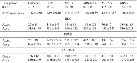
Table 2.Transport model results and ice core averages. In the first row the1t /τvalues of EDML vs. EDC for different time periods during the past 150 ka are shown. Below, the fluxes of nssCa2+(JnssCa) and ssNa+(JssNa) are indicated for EDC, EDML, and TALDICE, for the
corresponding time intervals (given in µg m−2a−1).
Time period Holocene LGM MIS 3 MIS 4–5.4 MIS 5.5 MIS 6
(ka BP) 3–15 15–30 30–60 60–115 115–133 133–146
1t /τ(EDML/EDC) 1.22±0.61 1.19±0.16 1.40±0.43 1.48±0.39 1.54±0.57 1.38±0.30
EDC
JnssCa 22±14 414±145 141±84 118±121 30±17 384±113
JssNa 515±134 786±142 866±112 830±161 455±187 816±205
EDML
JnssCa 76±49 1433±505 555±277 442±396 130±56 1559±519
JssNa 684±245 1802±332 1656±334 1536±310 761±417 1454±512
TALDICE
JnssCa 136±86 507±138 190±93 170±138 110±68 422±132
JssNa 850±309 1336±383 1750±323 1223±293 969±364 1279±158
core Fe measurements investigating T1 (Gaspari et al., 2006; Spolaor et al., 2013) which conclude that a reduction in iron fertilisation in the SO contributed up to 40 ppm to the CO2
increase during T1. Also an estimate based on Fe measure-ments in marine sedimeasure-ments constrains the effect of natural ae-olian iron deposition on marine export production in the SO region to up to 40 ppm of the atmospheric CO2concentration
changes during the last glacial cycle (Martínez-Garcia et al., 2011).
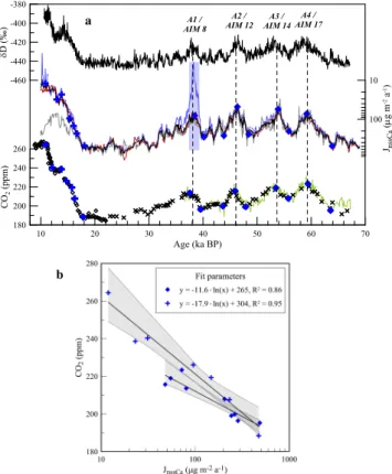
In order to calculate the spatially most representative record of dust deposition changes in the Antarctic/SO re-gion, we calculated a composite of the EDC, EDML, and TALDICE nssCa2+ records. Our composite nssCa2+ flux record uses the arithmetic average, however, with some ex-ceptions described in the following. EDML values were cor-rected for their offset compared to EDC and TALDICE. This was done by matching the logarithmic EDML values to those of EDC during the LGM (24–19 ka BP) when the common southern South American source was strongest, and then linearly shifting the entire EDML record according to the resulting offset. TALDICE values younger than 15 ka BP were discarded for the calculation because of their higher Holocene values compared to EDC and EDML reflecting the substantial contribution of local sources. During AIM 8 (A1) (i.e. 39.3–37.4 ka BP), the EDC values were discarded (see Fig. 5a). In Fig. 5b the linear regression of the com-posite nssCa2+ flux vs. atmospheric CO
2 is shown for T1
and for the period covering A1–A4 as done by Röthlisberger et al. (2004). Due to the omission of the low EDC nssCa2+ flux during AIM 8, our regression through the points cov-ering A1–A4 is much steeper compared to the one obtained by Röthlisberger et al. (2004). Following the argumentation of Röthlisberger et al. (2004), we conclude that the reduc-tion of iron supply through reduced aeolian dust deposireduc-tion over the SO may have contributed up to 40 ppm to the
at-mospheric CO2increase during T1, which is in line with the
results based on ice core Fe analyses of Gaspari et al. (2006).
3.4 Non-sea salt calcium and sea salt sodium during the last 150 000 years
3.4.1 Comparison of EDC versus EDML
In the following we compare different nssCa2+records us-ing our simple exponential transport model as described in Sect. 2.4. In this section we update a comparison study be-tween EDC and EDML done by Fischer et al. (2007a), while in the next section (Sect. 3.4.2) the comparison is extended to Vostok and the new TALDICE nssCa2+record.
10 20 30 40 50 60 70
Age (ka BP)
180 200 220 240 260
CO
2
(ppm)
100 10
JnssCa
(
g m
-2 a -1)
-460 -440 -420 -400 -380
A4 / AIM 17 A3 / AIM 14 A2 / AIM 12 A1 / AIM 8
a
b
Fig. 5. (a)Estimate of CO2sensitivity on dust changes. EDCδD is shown in the top panel, CO2concentrations from EDC (black open
diamonds) and Taylor Dome (black crosses) in the bottom panel.
More recent EDML and TALDICE CO2concentrations (Bereiter
et al., 2012) are shown for comparison (green line). The middle panel shows the mean nssCa2+ flux (JnssCa) calculated from the
100 yr medians of EDC, EDML, and TALDICE (black line); dis-carded EDC values during AIM 8 are marked by the blue shaded area. Blue diamonds and crosses in the bottom panel indicate the same tie points used for the linear regression calculation as done by Röthlisberger et al. (2004). In addition, the 100 yr means of EDC (blue line), offset-corrected EDML (red line), and TALDICE (grey line) are shown in the middle panel.(b)Linear regressions of the blue diamonds and crosses from(a), according to Röthlisberger et al. (2004). Due to the discarded EDC values during AIM 8 we obtain a regression line of the diamonds (representing CO2 and
nssCa2+during A4–A1) much closer to the one during T1,
indi-cated by the crosses. Grey shaded areas indicate the 95 % signifi-cance intervals.
and is therefore not providing a thorough correction, never-theless, it is seen that the IC blank contribution has a signif-icant effect, which biases the outcome of the investigations as already mentioned in Fischer et al. (2007a). Furthermore, if only data of the cold periods are investigated, the two data sets (IC and CFA nssCa2+) are in accordance with each other, resulting in the same linear regressions of the two plots (not shown).
When using CFA data it can only be seen that the offset 1t /τ has been constant over the whole period. The linear
fit through all data points reveals a slope of a= 1.02 with r2= 0.87 (total number of data pointsN= 1336). The offset 1t /τ during the Holocene is 1.22±0.65, during the LGM is it 1.19±0.16, thus virtually the same. This is
remark-able, since different glacial/interglacial variations in dust and other aerosol input have often been attributed to changes in wind speed and atmospheric circulation around Antarctica and, thus, to transport effects (e.g. Petit et al., 1990, 1999). Indeed there have been more recent studies, which suggest only moderate glacial/interglacial variations in wind speed and latitudinal shifts of the westerlies based on atmospheric circulation models (Krinner and Genthon, 1998, 2003; Ma-howald et al., 2006; Sime et al., 2013) as well as based on size distribution measurements of particulate dust in East Antarc-tic ice cores (Delmonte et al., 2004).
Based on our simple transport model, we cannot see any transport effects influencing atmospheric dust concentrations at the two drilling sites during the last 150 ka. Yet, chang-ing wind speeds (i.e. more efficient transport for colder cli-mate conditions) could still be compensated by simultane-ous changes ofτ. However, this would require decreased at-mospheric residence times during colder periods, although τ is suggested to be longer during colder conditions due to reduced wet deposition en route (Yung et al., 1996; Pe-tit et al., 1999; Lambert et al., 2008). Other studies high-light the spatially variable nature of dust lifetimes, which depend on the transport pathways (Albani et al., 2012b). In summary, based on our multi-site nssCa2+ flux records we conclude that transport intensity as well as atmospheric residence time plays a minor role for the observed dust flux changes on the East Antarctic plateau during the last two glacial/interglacial cycles. Instead, our transport model suggests source strength changes to be mainly responsi-ble for the pronounced nssCa2+ changes (EDC and EDML nssCa2+ flux ratio LGM/Holocene ≈18, see Table 2) on
the East Antarctic plateau as suggested by previous studies (e.g. Wolff et al., 2006; Fischer et al., 2007a).
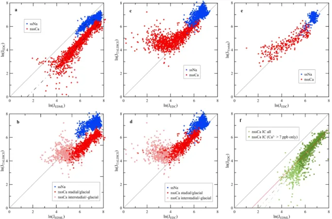
Fig. 6.Double-logarithmic scatter plots of the nssCa2+(red) and ssNa+(blue) fluxes in 100 yr resolution (500 yr resolution for Vostok only).
(a)EDC vs. EDML. The linear regression (dash-dotted line) shows a slope of 1 for nssCa2+and of 0.6 for ssNa+. Outliers of the AIM 8 event are indicated as red crosses (see text for explanation).(b)TALDICE vs. EDML. Cold (dark red dots) and warm periods (light red dots) are discriminated in the nssCa2+scatter plot.(c)TALDICE vs. EDC. The strong correlation of(a)is no longer persistent with these two ice cores when considering all climate periods of the past 150 ka.(d)TALDICE vs. EDC. The same data as in(c), however, cold (dark red dots) and warm periods (light red dots) are now discriminated. It becomes evident that during cold periods the linear correlation is still persistent, while for warm periods the two records are completely uncorrelated. EDC outliers during AIM 8 are indicated with red crosses.
(e)Vostok vs. EDC. Vostok data were analysed using IC, thus, low nssCa2+fluxes are biased towards higher values in the Vostok record. Data are shown in 500 yr resolution only.(f)EDML IC data versus EDC CFA data as shown in Fischer et al. (2007a). All data are shown in light green, in dark green only the data with original Ca2+concentrations higher than 7 ppb. Linear regressions (dash-dotted lines) through all the IC data (light green, slope of the regression 1.26) and those above the 7 ppb threshold only (dark green, slope 1.13) show that the IC data set is indeed approaching the slope of the CFA data set as in(a)(red line, slope 1.02), when low concentration IC values are discarded.
Australia during warmer periods. This is also discussed from a climate model point-of-view in Sect. 3.5.
The atmospheric lifetimeτof dust particles has been mod-elled to be of the order of 3–10 days by previous studies with no significant changes over glacial/interglacial changes (e.g. Yung et al., 1996; Mahowald et al., 1999; Werner et al., 2002; Tegen, 2003). The transport time for aerosol from the Atlantic sector of the East Antarctic ice sheet (EDML) to the EDC and TALDICE drilling sites according to the results of our transport model is in the range of 1.2–1.5 times the at-mospheric life time. This results in a transportation time of about 4–15 days in line with back trajectory studies (Reijmer et al., 2002; Scarchilli et al., 2011). In Table 2 we compiled 1t /τbetween EDML and EDC for the major climate periods over the last 150 ka. Interestingly,1t /τ gradually decreases
through time since the last interglacial period (see Table 2). However, it has to be acknowledged that these changes re-ported in Table 2 are small compared to the given standard deviation. Nevertheless, based on our ice core data we con-clude that changes in transport and residence times of terres-trial aerosol are not subject to strong temporal changes and change only slowly on millennial timescales.
texture, and weathering (Bigler et al., 2010; Wolff et al., 2006). Most of those are fast reacting parameters compared to millennial timescale changes and thus corroborate the hy-pothesis of source strength changes being mainly responsible for rapid changes in dust input on the East Antarctic ice sheet.
3.4.2 Comparison of TALDICE versus EDML, EDC, and Vostok
In contrast to the EDC/EDML comparison, the good linear relationship between the logarithms of the nssCa2+ fluxes breaks down for TALDICE (Fig. 6c). Especially for lower concentrations, i.e. warmer conditions, there is a bias towards higher values in TALDICE. For this reason we divided the data in two groups, one for warm climate conditions the other for cold climate conditions. As a threshold between the two groups an arbitrary value of−38.9 ‰ in theδ18O TALDICE record has been chosen (dashed line in the top panel of Fig. 3). In Fig. 6d the data shown in Fig. 6c are discrim-inated by thisδ18O threshold, resulting in two completely different regimes. While for cold climate conditions a linear relation between TALDICE and EDC exists (r2= 0.75, total number of data pointsN= 728), the two nssCa2+fluxes are completely uncorrelated (r2= 0.02, N= 588) during warm periods. A similar behaviour can be observed when compar-ing TALDICE and EDML with strongly correlated nssCa2+ fluxes during cold periods (r2= 0.77,N= 759) and no cor-relation during warm periods (r2= 5×10⁻⁶,N= 582) (see
Fig. 6b).
Furthermore, the calculated offset1t /τis close to zero for glacial conditions of TALDICE vs. EDC (Fig. 6d) indicating that the transport times to both drilling sites are almost equal (assuming the sameτ for both transport paths as well as the same source region). The same observation is valid for the comparison of EDC with Vostok (see Fig. 6e) for the entire past 150 ka. However, it has to be considered that the Vostok data have been analysed with IC and show the same signif-icant blank contribution for low Ca2+concentrations as the IC data of EDML, resulting in a bias towards higher values in the Vostok data for low values (see Fig. 6e).
An offset1t /τ close to zero for EDC vs. TALDICE as well as Vostok, respectively, is in agreement with studies based on back trajectories, which simulate the provenance of air parcels (Reijmer et al., 2002; Scarchilli et al., 2011) mostly originating from western pathways (dominated by the distinct Westerlies over the SO). However, recent simulations based on modern meteorological data suggest that a signifi-cant part of air masses to northern Victoria Land (i.e. Talos Dome) originate also from atypical pathways, i.e. southern and eastern pathways instead of the common western path-ways (Scarchilli et al., 2011; Delmonte et al., 2013).
Higher nssCa2+flux in TALDICE for warm climate con-ditions might also be explained by one or more additional local dust sources, which are only relevant for northern Vic-toria Land, but not for the East Antarctic plateau. Previous
studies on the isotopic signature (87Sr/86Sr andǫNd(0)) of
interglacial dust from plateau ice cores show matching char-acteristics with dust from the Antarctic dry valleys (Del-monte et al., 2007). More recent studies of the isotopic signa-tures of dust particles in TALDICE, on the other hand, show good agreement also with dust samples taken from the Mesa Range, Nunataks at the margin of the Antarctic plateau and close to Talos Dome (Delmonte et al., 2010a, b, 2013). How-ever, the identification of a local sub-region by isotopic sig-nature analyses of potential source areas is complicated due to the ubiquitous mixing of the TALDICE dust samples with volcanic particles (Delmonte et al., 2013).
While the geographical proximity and altitude favours the contribution of the Mesa Range, the source strength of the Antarctic dry valleys is much enhanced during warm peri-ods by glacial drift left behind from retreating glaciers, flu-vial erosion and frost weathering due to temperatures above 0◦C during the Antarctic summer. Furthermore, the ice-free areas in the Dry Valleys were substantially smaller or even completely covered by ice sheets during the last glacial pe-riod (Denton and Hughes, 2002; Huybrechts, 2002), which reduces the source strength drastically during these periods. As shown by Hall and Denton (2000) the Ross Sea was not only covered by an ice shelf during the LGM as it is to-day, but there was the Ross Sea Ice Sheet reaching down from the ground of the Ross Sea up into the Dry Valleys with an altitude of up to 350 m a.s.l. Johnson et al. (2008) have shown that the Cape Adare region (at the north east-ern edge of northeast-ern Victoria land) was completely ice cov-ered during the LGM and only became uncovcov-ered by ice at the transition into the Holocene at approx. 16 ka BP. In con-trast, the Mesa Range was not covered by ice for the last 2 Myr as reconstructed by Oberholzer et al. (2008) by dating of moraines and erratic blocs with cosmogenic nuclides, in-volving a more constant source strength of the Mesa Range over glacial–interglacial and stadial–interstadial cycles. It is also possible that the dust source of the Mesa Range is par-tially depleted due to its long exposition to the atmosphere leading to a limited availability of mobile dust. Nonetheless, the flux of particles at Talos Dome associated to the local sources was similar during the LGM and the early Holocene (Albani et al., 2012a). Thus, we suggest that both proximal regions (Antarctic dry valleys and Mesa Range) are potential local source regions for dust input to Talos Dome and dedi-cated tracer studies are needed to provide the final answer.
3.5 Verification of our transport model by climate model data
Fig. 7. (a)Dust column load of 1 yr tuned model runs at ice core grid points (Albani et al., 2012b). Double-logarithmic plots at EDML (red diamonds), Vostok (blue squares), and TALDICE (yellow tri-angles) vs. EDC.(b)Double-logarithmic plots of modelled dust de-position for all drill sites. The results are from the same model run as in(a).(c)Results of two 10 yr simulations showing inter-annual variability (10 points for each climate period) of the dust column load. Double-logarithmic scatter plots at EDML (red diamonds), Vostok (blue squares), and TALDICE (yellow triangles) vs. EDC, with the linear regressions including significance intervals (95 %) indicated in respective colours. See Table 2 for slopes, standard deviations, andr2values of the regressions shown in this figure.
(d)Double-logarithmic plots of two 10 yr simulations for all drill sites showing inter-annual variability of the dust deposition. The results are from the same model run as in(c). Linear regressions including significance intervals (95 %) are indicated in respective colours.(e)Double logarithmic scatter plot of the source mobili-sation vs. deposition showing the relation of dust deposited at the four ice core sites originating from a unique source (South Amer-ica, SAM) based on the 1 yr tuned case of Albani et al. (2012b). Green triangles represent EDC.
the source emissions in the model allows us to explore the source–transport–deposition relations in a consistent frame-work. Our model allows for investigating equilibrium simu-lations from two climate periods, i.e. the current climate (rep-resentative of the Holocene) and the LGM.
For the exponential transport model, we considered the flux of ice core aerosol proxy data representative of the atmo-spheric aerosol concentration at the drill sites (see Sect. 2.3). For the model results, we consider modelled dust deposition flux and dust load at the drilling sites. A version of the model with the best accuracy in reproducing ice core deposition (and source apportionment) is the 1 yr tuned case from Al-bani et al. (2012b). Tuning was halving Australian emissions for current climate, and doubling it for the LGM, compared to a companion couple of runs spanning 10 years. The tuning yielded a better fit to the data for both climates. The results of the 1-year tuned model run show a slope close to one for the four ice cores (Fig. 7a) and give the source apportionment of Fig. 3 in Albani et al. (2012b).
A very similar behaviour can be observed when comparing the model results in Fig. 7a with the ice core data in Fig. 6. EDC, Vostok, and TALDICE model data show one-to-one relationships, with EDC and Vostok exhibiting a very small 1t /τoffset, thus exhibiting a nearly one-to-one relationship. Higher dust load for TALDICE and in particular for EDML (due to its proximity to the main source areas in southern South America) result in a distinct offset compared to EDC and Vostok, for both climate periods as also observed in the ice core data as well. In addition, the slope of the model re-sults for EDML shows a slightly higher value.
If we now consider dust deposition instead of atmospheric surface concentration of the very same model run (Fig. 7b), we see all the regression lines having slopes close to one, but more distinct offsets. The uncertainty of the regression is unconstrained, as we are just using two points (average for current climate and LGM). Nevertheless, if we compare the 10 yr simulation using the same model but a different spatial pattern of emissions from the main source areas (Fig. 7d) with the 1 yr run of the very same simulation (not shown), we can infer that the slopes of the tuned 1 yr simulations are representative of the modelled relations, even though they are not the same for the tuned and the untuned version. Using the 10 yr runs results in slightly more scattered slopes for both dust load (Fig. 7c) and deposition flux (Fig. 7d), but allows for an estimation of the error andr2of the regression lines (in Table 3 the slopes, standard deviations, andr2values for all regressions shown in Fig. 7 are indicated).
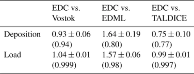
Table 3.Slopes of the linear regressions calculated for the 10 yr model runs as shown in Fig. 7. The first line indicates the slopes of the dust deposition (dep.) (Fig. 7d), the second line those of the atmospheric dust load (Fig. 7c). The slopes of the regressions are indicated including the standard deviation, the respectiver2values are indicated in parenthesis.
EDC vs. EDC vs. EDC vs.
Vostok EDML TALDICE
Deposition 0.93±0.06 1.64±0.19 0.75±0.10
(0.94) (0.80) (0.77)
Load 1.04±0.01 1.57±0.06 0.99±0.01
(0.999) (0.98) (0.997)
precipitation rates, on the regression line is much smaller in the ice core data, as it represents only about a tenth of all data points used in the regression, while it represents 50 % of the data points defining the regression lines in Fig. 7. This effect may be partly responsible for the difference in the slope be-tween data and model for EDML. Based on the overall good correspondence of the slopes of the regression lines for atmo-spheric dust loadings in Fig. 7a and c, we conclude that our transport model appears to be able to describe the transport effect on dust concentrations in different regions on the East Antarctic ice sheet.
The differences between the slopes in the modelled dust load and deposition (compare Fig. 7a/c with b/d) reflect the deposition processes in the model. For our exponential-decay transport model applied on the ice core flux data we only as-sume dry deposition (see Sect. 2.3), which is a reasonable ap-proximation for interior sites such as EDC and Vostok (Wolff et al., 2006) and for all sites in the glacial, where snow ac-cumulation was about 50 % lower than today, but may be in-adequate in the case of peripheral sites such as EDML and Talos Dome for recent accumulation rate conditions. On the other hand, the Mahowald et al. (2006) model simulates both dry and wet deposition in proportions that are well repre-sented for coastal Antarctic sites, but likely overestimate the contribution of wet deposition on the plateau (Albani et al., 2012b), thus leading to much larger differences in the loga-rithmic deposition fluxes in EDML and Talos Dome relative to EDC than in the modelled atmospheric concentrations.
A comparison of the ice core data1t /τ offsets reported in Table 2 and shown in Fig. 6 with modelled ones (Fig. 7b and d) indicates that the modelled deposition is biased to-ward higher values for TALDICE and EDML, possibly in relation to overestimated precipitation rates in the model (Al-bani et al., 2012b). However, since the glacial/interglacial in-crease in snow deposition of a factor two is well captured by the model (Albani et al., 2012b), the one-to-one relation-ship is well reproduced, so there is a solid base to discuss the model results in comparison with the observations and making inferences on the underlying mechanisms, based on model physics.
With the model we can also explore the relation between source emissions from a specific area and the dust deposi-tion. Considering emission and dust deposition from South America alone (Fig. 7e) gives a one-to-one relationship be-tween logarithmic emission and deposition for all ice cores (only TALDICE has also a major Australian contribution in the model). This result is not surprising considering that the source experiencing the largest changes in modelled emis-sions is South America, with a factor 13 compared to a factor four for Australia (Albani et al., 2012b). In addition, the rela-tive abundance of Patagonian dust for modelled dust deposi-tion at ice core sites is either dominant (EDML) or increasing in the LGM for the other sites. Therefore, it is not surprising that southern South America is driving the slope, and may be the reason why the approximation of a unique source im-plicit in the exponential transport model holds in reproducing the one-to-one relationship, despite the observed complexity of the dust provenance mix especially in the Holocene (see Introduction).
The reason why the logarithms of TALDICE vs. EDC dust deposition in the model show a one-to-one relationship, which is not consistent with the ice core data due to the strong contribution of local sources at Talos Dome during the Holocene (see Sect. 3.4.2), is because the model does not consider local (Antarctic) sources. Thus, this particular fea-ture in Talos Dome ice core data cannot be capfea-tured in the model.
cores in Antarctica (Albani et al., 2012b). Future improved model studies will help to better disentangle the source and transport contributions to glacial–interglacial dust changes in Antarctica.
4 Conclusions
In this study we presented new CFA nssCa2+ and ssNa+ records of the Talos Dome ice core in centennial resolu-tion reaching back 150 ka BP. TALDICE nssCa2+flux shows both large-scale changes on glacial/interglacial timescales as well as a regional signal, emerging when dust advection from remote sources was extremely low, that is, during warm (in-terglacial) periods. Dust deposition at Talos Dome generally reflects major climate changes on a hemispheric scale dur-ing the last 150 ka. However, the significant contribution of proximal dust sources during warm climate periods (e.g. the Holocene) makes Talos Dome sensitive to regional atmo-spheric circulation changes.
Our new nssCa2+and ssNa+flux records corroborate the scenario proposed by Albani et al. (2012a), suggesting that more frequent air mass trajectories through the Ross Sea are mainly responsible for a reduced dust input from local sources after 8 ka BP. Since there are no TALDICE nssCa2+ and ssNa+ data available for the late Holocene, we cannot examine the behaviour of the two parameters in the context of a late Holocene Ross ice shelf re-advance (Albani et al., 2012a). An extension of the existing records to the last three millennia would allow for a verification of an according be-haviour. Nevertheless, based on the new TALDICE mineral dust and sea ice proxy records we suggest similar regional climate conditions as observed during the Holocene prevail-ing also durprevail-ing the last interglacial period in the Ross Sea area. In particular, our new ssNa+data indicate the presence of extended sea ice cover in the Ross Sea area during MIS 5.5 of similar extent as during the Holocene.
Two potential local source regions, the Antarctic dry val-leys and/or the Mesa Range, which could not been discrim-inated unambiguously as main contributors to local dust in-put to Talos Dome so far, may contribute to the higher dust fluxes during warm periods compared to the other ice core sites. The Dry Valleys are considered to be an efficient dust source because glacial drift deposits, fluvial erosion, and frost weathering enhance the availability of mobile dust dur-ing warm periods, while durdur-ing cold periods this source re-gion is ice covered and thus no longer active in line with our new TALDICE nssCa2+data. On the other hand, sources in the Mesa Range lie at high elevation and much closer to the site. They are smaller compared to the Dry Valleys and pos-sibly in part depleted because of the long exposure, but at the same time they were ice free throughout the glacial period, consistent with the dust coarse particle flux (Albani et al., 2012a).
The availability of three highly resolved nssCa2+records (EDC, EDML, and TALDICE, respectively) allow for a re-vision of the estimate on atmospheric CO2 sensitivity to
dust induced iron fertilisation in the SO. Röthlisberger et al. (2004) based their estimation on the only record available at that time (CFA nssCa2+ of EDC) including extremely low values during AIM 8 which, however, have not been ob-served in other ice core records. Accordingly, their finding of 20 ppm seems to underestimate the CO2sensitivity. In a
revised estimation, including nssCa2+of TALDICE, EDML, and EDC, and discarding the extreme low EDC values during AIM 8, we estimate the increase of atmospheric CO2during
T1 linked to reduced dust induced iron fertilisation in the SO to be up to 40 ppm.
Based on our exponential transport model applied on nssCa2+ records of four East Antarctic ice cores we cannot see any long range transport effects influencing atmospheric dust concentration changes in East Antarctica. A compari-son with climate model results confirm our findings of con-stant transport efficiencies (i.e.1t /τ) for dust fluxes at the four drill sites for Holocene/LGM climate. The model, how-ever, allows that the one-to-one relationship of dust fluxes at the four drill sites would be also consistent with a more complex scenario where transport changes are compensated by a changing source mix. Nevertheless, we can conclude that the observed nssCa2+ flux changes predominantly re-flect changes in southern South America source strength dur-ing the past 150 ka. Changdur-ing transport time and atmospheric residence time may have contributed to determining the mag-nitude of the observed flux changes.
Supplementary material related to this article is
available online at http://www.clim-past.net/9/2789/2013/ cp-9-2789-2013-supplement.zip.
Acknowledgements. We thank the AWI team, in particular Anna Wegner and Birthe Twarloh, as well as Matthias Bigler and Christof Bernhard for their support during the CFA analyses. This research is funded by the Swiss National Science Foundation and the Prince Albert II of Monaco foundation. The Talos Dome Ice core Project (TALDICE), a joint European programme, is funded by national contributions from Italy, France, Germany, Switzerland and the UK. Primary logistical support was provided by PNRA at Talos Dome. This is TALDICE publication no. 35.
Edited by: E. Isaksson
References
Albani, S., Delmonte, B., Maggi, V., Baroni, C., Petit, J.-R., Stenni, B., Mazzola, C., and Frezzotti, M.: Interpreting last glacial to Holocene dust changes at Talos Dome (East Antarctica): im-plications for atmospheric variations from regional to hemi-spheric scales, Clim. Past, 8, 741–750, doi:10.5194/cp-8-741-2012, 2012a.
Albani, S., Mahowald, N., Delmonte, B., Maggi, V., and Winckler, G.: Comparing modeled and observed changes in mineral dust transport and deposition to Antarctica between the Last Glacial Maximum and current climates, Clim. Dynam., 38, 1731–1755, doi:10.1007/s00382-011-1139-5, 2012b.
Archer, D., Winguth, A., Lea, D., and Mahowald, N.: What caused the glacial/interglacial atmospheric pCO2 cycles?, Rev. Geo-phys., 38, 159–189, doi:10.1029/1999rg000066, 2000.
Basile, I., Grousset, F. E., Revel, M., Petit, J. R., Biscaye, P. E., and Barkov, N. I.: Patagonian origin of glacial dust deposited in East Antarctica (Vostok and Dome C) during glacial stages 2, 4 and 6, Earth Planet. Sc. Lett., 146, 573–589, doi:10.1016/S0012-821X(96)00255-5, 1997.
Bazin, L., Landais, A., Lemieux-Dudon, B., Toyé Mahamadou Kele, H., Veres, D., Parrenin, F., Martinerie, P., Ritz, C., Capron, E., Lipenkov, V., Loutre, M.-F., Raynaud, D., Vinther, B., Svens-son, A., Rasmussen, S. O., Severi, M., Blunier, T., Leuenberger, M., Fischer, H., Masson-Delmotte, V., Chappellaz, J., and Wolff, E.: An optimized multi-proxy, multi-site Antarctic ice and gas or-bital chronology (AICC2012): 120–800 ka, Clim. Past, 9, 1715– 1731, doi:10.5194/cp-9-1715-2013, 2013.
Bereiter, B., Lüthi, D., Siegrist, M., Schüpbach, S., Stocker, T. F., and Fischer, H.: Mode change of millennial CO2 vari-ability during the last glacial cycle associated with a bipolar marine carbon seesaw, P. Natl. Acad. Sci., 109, 9755–9760, doi:10.1073/pnas.1204069109, 2012.
Bigler, M., Röthlisberger, R., Lambert, F., Stocker, T. F., and Wagenbach, D.: Aerosol deposited in East Antarctica over the last glacial cycle: Detailed apportionment of continental and sea-salt contributions, J. Geophys. Res., 111, D08205, doi:10.1029/2005JD006469, 2006.
Bigler, M., Röthlisberger, R., Lambert, F., Wolff, E. W., Castel-lano, E., Udisti, R., Stocker, T. F., and Fischer, H.: Atmospheric decadal variability from high-resolution Dome C ice core records of aerosol constituents beyond the Last Interglacial, Quaternary Sci. Rev., 29, 324–337, doi:10.1016/j.quascirev.2009.09.009, 2010.
Blunier, T., Schwander, J., Stauffer, B., Stocker, T., Dällenbach, A., Indermühle, A., Tschumi, J., Chappellaz, J., Raynaud, D., and Barnola, J. M.: Timing of the Antarctic Cold Re-versal and the atmospheric CO2 increase with respect to the Younger Dryas event, Geophys. Res. Lett., 24, 2683–2686, doi:10.1029/97GL02658, 1997.
Bory, A., Wolff, E., Mulvaney, R., Jagoutz, E., Wegner, A., Ruth, U., and Elderfield, H.: Multiple sources supply eolian mineral dust to the Atlantic sector of coastal Antarctica: Evidence from recent snow layers at the top of Berkner Island ice sheet, Earth Planet. Sc. Lett., 291, 138–148, doi:10.1016/j.epsl.2010.01.006, 2010.
Bouttes, N., Paillard, D., and Roche, D. M.: Impact of brine-induced stratification on the glacial carbon cycle, Clim. Past, 6, 575–589, doi:10.5194/cp-6-575-2010, 2010.
Brook, E. J., White, J. W. C., Schilla, A. S. M., Bender, M. L., Bar-nett, B., Severinghaus, J. P., Taylor, K. C., Alley, R. B., and Steig, E. J.: Timing of millennial-scale climate change at Siple Dome, West Antarctica, during the last glacial period, Quaternary Sci. Rev., 24, 1333–1343, doi:10.1016/j.quascirev.2005.02.002, 2005.
Buiron, D., Chappellaz, J., Stenni, B., Frezzotti, M., Baumgart-ner, M., Capron, E., Landais, A., Lemieux-Dudon, B., Masson-Delmotte, V., Montagnat, M., Parrenin, F., and Schilt, A.: TALDICE-1 age scale of the Talos Dome deep ice core, East Antarctica, Clim. Past, 7, 1–16, doi:10.5194/cp-7-1-2011, 2011. De Angelis, M., Steffensen, J. P., Legrand, M., Clausen, H., and Hammer, C.: Primary aerosol (sea salt and soil dust) deposited in Greenland ice during the last climatic cycle: Comparison with east Antarctic records, J. Geophys. Res.-Oceans, 102, 26681– 26698, doi:10.1029/97jc01298, 1997.
Delmonte, B., Petit, J. R., Basile-Doelsch, I., Jagoutz, E., and Maggi, V.: Developments in Quaternary Sciences, vol. 7, chap. 6: Late quaternary interglacials in East Antarctica from ice-core dust records, Elsevier, 53–73, 2007.
Delmonte, B., Andersson, P. S., Hansson, M., Schöberg, H., Pe-tit, J. R., Basile-Doelsch, I., and Maggi, V.: Aeolian dust in East Antarctica (EPICA-Dome C and Vostok): Provenance dur-ing glacial ages over the last 800 kyr, Geophys. Res. Lett., 35, L07703, doi:10.1029/2008GL033382, 2008.
Delmonte, B., Andersson, P. S., Schöberg, H., Hansson, M., Pe-tit, J. R., Delmas, R., Gaiero, D. M., Maggi, V., and Frez-zotti, M.: Geographic provenance of aeolian dust in East Antarc-tica during Pleistocene glaciations: preliminary results from Talos Dome and comparison with East Antarctic and new Andean ice core data, Quaternary Sci. Rev., 29, 256–264, doi:10.1016/j.quascirev.2009.05.010, 2010a.
Delmonte, B., Baroni, C., Andersson, P. S., Schöberg, H., Hansson, M., Aciego, S., Petit, J. R., Albani, S., Mazzola, C., Maggi, V., and Frezzotti, M.: Aeolian dust in the Talos Dome ice core (East Antarctica, Pacific/Ross Sea sector): Victoria Land versus remote sources over the last two climate cycles, J. Quaternary Sci., 25, 1327–1337, doi:10.1002/jqs.1418, 2010b.
Delmonte, B., Baroni, C., Andersson, P. S., Narcisi, B., Salva-tore, M. C., Petit, J. R., Scarchilli, C., Frezzotti, M., Albani, S., and Maggi, V.: Modern and Holocene aeolian dust vari-ability from Talos Dome (Northern Victoria Land) to the inte-rior of the Antarctic ice sheet, Quaternary Sci. Rev., 64, 76–89, doi:10.1016/j.quascirev.2012.11.033, 2013.
Denton, G. H. and Hughes, T. J.: Reconstructing the Antarctic Ice Sheet at the Last Glacial Maximum, Quaternary Sci. Rev., 21, 193–202, doi:10.1016/S0277-3791(01)00090-7, 2002.
Dieckmann, G. S. and Hellmer, H. H.: The Importance of Sea Ice: An Overview, Wiley-Blackwell, 1–22, 2010.
EPICA, C. M.: Eight glacial cycles from an Antarctic ice core, Na-ture, 429, 623–628, doi:10.1038/nature02599, 2004.
EPICA, C. M.: One-to-one coupling of glacial climate vari-ability in Greenland and Antarctica, Nature, 444, 195–198, doi:10.1038/nature05301, 2006.
M.-L., Steffensen, J. P., Barbante, C., Gaspari, V., Gabrielli, P., and Wagenbach, D.: Reconstruction of millennial changes in dust emission, transport and regional sea ice coverage us-ing the deep EPICA ice cores from the Atlantic and Indian Ocean sector of Antarctica, Earth Planet. Sc. Lett., 260, 340–354, doi:10.1016/j.epsl.2007.06.014, 2007a.
Fischer, H., Siggaard-Andersen, M.-L., Ruth, U., Röthlisberger, R., and Wolff, E. W.: Glacial/interglacial changes in mineral dust and sea-salt records in polar ice cores: Sources, transport, and deposi-tion, Rev. Geophys., 45, RG1002, doi:10.1029/2005RG000192, 2007b.
Fischer, H., Schmitt, J., Lüthi, D., Stocker, T. F., Tschumi, T., Parekh, P., Joos, F., Köhler, P., Völker, C., Gersonde, R., Bar-bante, C., Le Floch, M., Raynaud, D., and Wolff, E.: The role
of Southern Ocean processes in orbital and millennial CO2
variations – A synthesis, Quaternary Sci. Rev., 29, 193–205, doi:10.1016/j.quascirev.2009.06.007, 2010.
Frezzotti, M., Urbini, S., Proposito, M., Scarchilli, C., and Gan-dolfi, S.: Spatial and temporal variability of surface mass bal-ance near Talos Dome, East Antarctica, J. Geophys. Res., 112, F02032, doi:10.1029/2006jf000638, 2007.
Gabrielli, P., Wegner, A., Petit, J. R., Delmonte, B., De Deck-ker, P., Gaspari, V., Fischer, H., Ruth, U., Kriews, M., Boutron, C., Cescon, P., and Barbante, C.: A major glacial-interglacial change in aeolian dust composition inferred from Rare Earth Elements in Antarctic ice, Quaternary Sci. Rev., 29, 265–273, doi:10.1016/j.quascirev.2009.09.002, 2010.
Gaiero, D. M.: Dust provenance in Antarctic ice during glacial pe-riods: From where in southern South America?, Geophys. Res. Lett., 34, L17707, doi:10.1029/2007gl030520, 2007.
Gaspari, V., Barbante, C., Cozzi, G., Cescon, P., Boutron, C. F., Gabrielli, P., Capodaglio, G., Ferrari, C., Petit, J. R., and Del-monte, B.: Atmospheric iron fluxes over the last deglacia-tion: Climatic implications, Geophys. Res. Lett., 33, L03704, doi:10.1029/2005gl024352, 2006.
Gersonde, R., Crosta, X., Abelmann, A., and Armand, L.: Sea-surface temperature and sea ice distribution of the
Southern Ocean at the EPILOG Last Glacial
Maxi-mum—a circum-Antarctic view based on siliceous
mi-crofossil records, Quaternary Sci. Rev., 24, 869–896,
doi:10.1016/j.quascirev.2004.07.015, 2005.
Hall, B. L. and Denton, G. H.: Extent and Chronology of the Ross Sea Ice Sheet and the Wilson Piedmont Glacier along the Scott Coast at and since the Last Glacial Maximum, Geogr. Ann. A, 82, 337–363, doi:10.1111/j.0435-3676.2000.00128.x, 2000. Huybrechts, P.: Sea-level changes at the LGM from ice-dynamic
reconstructions of the Greenland and Antarctic ice sheets dur-ing the glacial cycles, Quaternary Sci. Rev., 21, 203–231, doi:10.1016/S0277-3791(01)00082-8, 2002.
Johnson, J. S., Hillenbrand, C.-D., Smellie, J. L., and Roc-chi, S.: The last deglaciation of Cape Adare, northern
Victoria Land, Antarctica, Antarct. Sci., 20, 581–587,
doi:10.1017/S0954102008001417, 2008.
Jouzel, J., Masson-Delmotte, V., Cattani, O., Dreyfus, G., Falourd, S., Hoffmann, G., Minster, B., Nouet, J., Barnola, J. M., Chap-pellaz, J., Fischer, H., Gallet, J. C., Johnsen, S., Leuenberger, M., Loulergue, L., Lüthi, D., Oerter, H., Parrenin, F., Raisbeck, G., Raynaud, D., Schilt, A., Schwander, J., Selmo, E., Souchez, R., Spahni, R., Stauffer, B., Steffensen, J. P., Stenni, B., Stocker,
T. F., Tison, J. L., Werner, M., and Wolff, E. W.: Orbital and Mil-lennial Antarctic Climate Variability over the Past 800,000 Years, Science, 317, 793–796, doi:10.1126/science.1141038, 2007. Kaufmann, P. R., Federer, U., Hutterli, M. A., Bigler, M.,
Schüp-bach, S., Ruth, U., Schmitt, J., and Stocker, T. F.: An Improved Continuous Flow Analysis System for High-Resolution Field Measurements on Ice Cores, Environ. Sci. Technol., 42, 8044– 8050, doi:10.1021/es8007722, 2008.
Kaufmann, P. R., Fundel, F., Fischer, H., Bigler, M., Ruth, U., Ud-isti, R., Hansson, M., de Angelis, M., Barbante, C., Wolff, E. W., Hutterli, M. A., and Wagenbach, D.: Ammonium and non-sea salt sulfate in the EPICA ice cores as indicator of biological ac-tivity in the Southern Ocean, Quaternary Sci. Rev., 29, 313–323, doi:10.1016/j.quascirev.2009.11.009, 2010.
Knorr, G. and Lohmann, G.: Southern Ocean origin for the resump-tion of Atlantic thermohaline circularesump-tion during deglaciaresump-tion, Na-ture, 424, 532–536, doi:10.1038/nature01855, 2003.
Krinner, G. and Genthon, C.: GCM simulations of the Last Glacial Maximum surface climate of Greenland and Antarctica, Clim. Dynam., 14, 741–758, doi:10.1007/s003820050252, 1998. Krinner, G. and Genthon, C.: Tropospheric transport of
continen-tal tracers towards Antarctica under varying climatic conditions, Tellus B, 55, 54–70, doi:10.1034/j.1600-0889.2003.00004.x, 2003.
Lambert, F., Delmonte, B., Petit, J. R., Bigler, M., Kaufmann, P. R., Hutterli, M. A., Stocker, T. F., Ruth, U., Steffensen, J. P., and Maggi, V.: Dust-climate couplings over the past 800,000 years from the EPICA Dome C ice core, Nature, 452, 616–619, doi:10.1038/nature06763, 2008.
Lemieux-Dudon, B., Blayo, E., Petit, J.-R., Waelbroeck, C., Svens-son, A., Ritz, C., Barnola, J.-M., Narcisi, B. M., and Parrenin, F.: Consistent dating for Antarctic and Greenland ice cores, Qua-ternary Sci. Rev., 29, 8–20, doi:10.1016/j.quascirev.2009.11.010, 2010.
Li, F., Ginoux, P., and Ramaswamy, V.: Distribution, transport, and deposition of mineral dust in the Southern Ocean and Antarctica: Contribution of major sources, J. Geophys. Res. Atmos., 113, D10207, doi:10.1029/2007jd009190, 2008.
Mahowald, N. M., Kohfeld, K., Hansson, M., Balkanski, Y., Har-rison, S. P., Prentice, I. C., Schulz, M., and Rodhe, H.: Dust sources and deposition during the last glacial maximum and cur-rent climate: A comparison of model results with paleodata from ice cores and marine sediments, J. Geophys. Res.-Atmos., 104, 15895–15916, doi:10.1029/1999jd900084, 1999.
Mahowald, N. M., Muhs, D. R., Levis, S., Rasch, P. J., Yoshioka, M., Zender, C. S., and Luo, C.: Change in atmospheric mineral aerosols in response to climate: Last glacial period, preindustrial, modern, and doubled carbon dioxide climates, J. Geophys. Res.-Atmos., 111, D10202, doi:10.1029/2005jd006653, 2006. Marino, F., Castellano, E., Nava, S., Chiari, M., Ruth, U., Wegner,
A., Lucarelli, F., Udisti, R., Delmonte, B., and Maggi, V.: Co-herent composition of glacial dust on opposite sides of the East Antarctic Plateau inferred from the deep EPICA ice cores, Geo-phys. Res. Lett., 36, L23703, doi:10.1029/2009gl040732, 2009. Martin, J. H.: Glacial-interglacial CO2change: The Iron
Hypothe-sis, Paleoceanography, 5, 1–13, doi:10.1029/PA005i001p00001, 1990.