The FEMM Package: A Simple, Fast, and Accurate Open Source Electromagnetic Tool in Science and Engineering

Journal of Engineering Science and Technology Review 1 (2008) 83-89 Lecture Note

The FEMM Package: A Simple, Fast, and Accurate Open Source Electromagnetic

Tool in Science and Engineering

K. B. Baltzis

*

RadioCommunications Laboratory, Section of Applied and Environmental Physics,Dept. of Physics, Aristotle University of Thessaloniki, 54124, Thessaloniki, Hellas

Received 7 April 2008; Accepted 17 November 2008

___________________________________________________________________________________________

Abstract

The finite element method (FEM) is one of the most successful computational techniques for obtaining approximate solutions to the partial differential equations that arise in many scientific and engineering applications. Finite Element Method Magnetics (FEMM) is a software package for solving electromagnetic problems using FEM. The program addresses 2D planar and 3D axisymmetric linear and nonlinear harmonic low frequency magnetic and magnetostatic problems and linear electrostatic problems. It is a simple, accurate, and low computational cost open source product, popular in science, engineering, and education. In this paper the main characteristics and functions of the package are presented. In order to demonstrate its use and exhibit the aid it offers in the study of electromagnetics a series of illustrative examples are given. The aim of the paper is to demonstrate the capability of FEMM to meet as a complementary tool the needs of science and technology especially when factors like the economic cost or the software complexity do not allow the use of commercial products.

Keywords: Electromagnetics, simulation, finite element method, open source software.

___________________________________________________________________________________________

ρ ε

∇ ⋅ −

=

______________

©

J

estr

JOURNAL OF Engineering Science and

Technology Review

www.jestr.org

1. Introduction

The finite element method (FEM) is a computational method that can be applied to obtain solutions to a variety of problems in engineering and science. Steady, transient, linear and nonlinear problems in electromagnetics, structural analysis, and fluid dynamics may be analyzed and solved with it, [1-3]. It combines geometrical adaptability and material generality for modeling arbitrary geometries and materials of any composition without a need to alter the formulation of the computer code that implements it. The idea of the method is to divide the problem domain into a large number of subdomains, called finite elements, each with a simple geometry resulting in the transformation of the initial problem from a small but difficult to solve into a big but an easy to solve. Through the process of discretization (also referred to as meshing) a linear algebraic system with many unknowns is formed. However, algorithms exist that allow the resulting problem to be solved, usually in a short amount of time. In the electromagnetics a discretization scheme, such as the one that FEM implies, which implicitly incorporates most of the theoretical features of the problem under analysis is one of the best solutions to get accurate results in a variety of problems.

Finite Element Method Magnetics (FEMM) software package, [4], has been developed for this reason addressing some limiting cases of Maxwell’s equations. The magnetic problems faced are magnetostatic or the low frequency (LF) ones in which displacement currents are negligible. The

electrostatics solver considers the cases in which the magnetic field is neglected. The program addresses 2D planar and 3D axisymmetric linear and nonlinear harmonic magnetic and magnetostatic as well linear electrostatic problems. It is an open source, simple, accurate, and low computational cost open source product with several applications in electromagnetics, materials science, industry, medicine, experimental and particle physics, robotics, astronomy, space engineering, and education, e.g. [5-14]. In this paper it will be shown that FEMM is a useful tool for an in–depth study of electromagnetics, suitable for scientists and engineers.

The paper is organized as follows. In Section II some discussion about electromagnet theory and the basic principles of the finite element method is made. The main characteristics of FEMM are presented in Section III. In order to point out the evolutionary features of the software illustrative examples are given in Section IV. Finally, in Section VI conclusions are drawn.

2. Theoretical Backround

The electromagnetic field is expressed in terms of the electric field intensity

E

, the magnetic field flux density , and the current density , using the Maxwell’s equations. These are, [15-16]:

B

J

0

ρ ε

∇ ⋅ −

E

=

(1)

______________

* E-mail address kmpal@physics.auth.gr

ISSN: 1791-2377 © 2008 Kavala Institute of Technology. All rights reserved.

0

∇ ⋅ =

B

(2)

0

t

∂

∇× +

=

∂

B

E

(3)

0

t

μ

⎛

ε

∂

⎞

∇× −

_⎜

+

_⎟

=

∂

⎝

⎠

E

B

J

(4)

where

ρ

is the charge density, while

ε

and

μ

are respectively the electrical permittivity and the magnetic permeability of the medium. Quantities and are also related (Ohm’s law). It is:

E

J

σ

=

J

E

(5)

with

σ

the medium conductivity.

The FEMM package, [4], [17-18], addresses some limiting cases of Maxwell’s equations, the magnetostatics, the electrostatics, and the LF time harmonic magnetic problems. For the time–invariant cases (3) and (4) are simplified into:

0

∇× =

E

(6)

0

μ

∇× −

B

J

=

(7)

In a magnetostatic problem FEMM goes about finding a field that satisfies (2) and (7) via the magnetic vector potential approach. Flux density is written in terms of the vector potential

A

, as:

def

=

∇×

B

A

(8)

and Eq. (7) becomes:

( )

1

μ

⎛

⎞

∇×

_⎜⎜

∇×

=

⎝

B

A

⎠

⎟⎟

J

(9)

Which for the case of a linear isotropic magnetic material, [19], it is further simplified into

2

0

μ

∇

A

+

J

=

(10)

In an electrostatic problem FEMM employs the electric scalar potential

V

, defined from

def

=

− ∇

V

E

(11)

In this case the differential equation solved is the

2

0

V

ρ

ε

∇ +

=

(12)

Low frequency time harmonic magnetic problems are also solved with FEMM when the field is oscillating in one fixed frequency

ω

. In this case the equation solved is:

( )

1

0

eff

V

j

σ

ωσ

μ

∧

⎛

⎞

∇×

⎜

_⎜

∇×

⎟

_⎟

+ ∇ − +

⎝

B

α

⎠

J

α

=

(13)

where

∧

J

is the phasor transform of the applied current sources,

μ

_eff

( )

B

is the effective magnetic permeability, and is the complex amplitude of the phasor transformation, [20] , of .

α

A

In any electromagnetic problem a unique solution is guaranteed by the boundary conditions applied, [15-16]. The conditions used by FEMM are the Dirichlet, the Neumann, and the Robin. In the first, the potential is explicitly defined on the boundary. This is used in magnetic problems to keep magnetic flux from crossing the boundary and in electrostatics to fix the voltage of a surface in the problem domain. The second specifies the normal derivative of potential along the boundary and is consistent with an interface with a highly permeable metal. The last one is a linear combination of the previous two and is used to define boundary conditions that allow a bounded domain to mimic the behavior of an unbounded one. It usually denotes an interface with a material subject to eddy currents, [21-23], at frequencies where the material skin depth is very small.

As it is already mentioned FEM is used in many fields of science and engineering to obtain approximate solutions for the partial differential equations to be solved. Its basic concept is that although the behavior of a function may be complex when viewed over a large region, a simple approximation may be sufficed for a small subregion. In practice, it utilizes a variational problem that involves an integral of the differential equation over the problem domain by dividing it into a large number of non–overlapping subregions, each with a simple geometry. Over each subregion the solution of the partial differential equation is approximated by a polynomial function. These polynomials have to be pieced together so that where the edges of adjoining elements overlap the field representations must agree to maintain continuity of the field. Then the variational integral is evaluated as a sum of contributions from each element resulting in an algebraic system with a finite size than the original infinite–dimensional partial differential equation. When enough small regions are used the approximate solution closely matches the exact one. The advantage of breaking the domain down into a number of small elements is the problem transformation from a small but too complex into a big but relatively easy to solve. It has to be noticed that, unlike other computational techniques, in the finite element method the approximate solution is known throughout the domain as a pieceise function and not as a set of points.

3.The main characteristics of the package

extension language, [24-25], used to add scripting/batch processing facilities to FEMM. It is divided into three parts:

• The interactive shell (femm.exe), a multiple document interface pre-processor and a post-processor for the problems solved by the package.

• The triangle.exe which segments the problem domain into a large number of triangles.

• The solvers (fkern.exe for magnetics and belasolv for electrostatics). These take a set of data files that describe the problem and solve Maxwell’s equations to obtain values for the desired field throughout the problem domain. It has to be noticed that the value of potential in each triangle is approximated from the linear interpolation of its values at its three vertices.

4. Examples and discussions

To demonstrate the characteristics and capabilities of FEMM a series of illustrative examples are presented here. However a further analysis of the results is out of the scope of the paper. Three problems are studied, a magnetostatic, an LF time harmonic magnetic and an electrostatic one. The first example is described in detail in order to make clear the characteristics of the software. The steps followed in each case are:

I. Physical problem description. II. Model design.

III. Boundaries definition. IV. Materials description.

V. Boundary conditions application. VI. Mess generation.

VII. Finite Element Method application. VIII.Results extraction and analysis.

FEMM software and its applications can be evolutive in the sense that the offered tools are of various levels of complexity. It quiet easy for someone to tackle, step by step, depending on his apprenticeship level, various tools adapted to the solving of problems of increasing complexity.

Example 1: Calculation of the magnetic field of an air– cored solenoid in open space.

An air–cored solenoid in open space with an inner diameter of 1 inch, an outer diameter of 3 inches, and an axial length of 2 inches is considered, see Fig. 1. The coil is built out of 100 turns of copper wire. A DC current of 1A is flowing through the wire.

z

- axis

I=1A

Air

Copper

Fig. 1. Air–cored coil geometry.

The problem is a magnetostatic axisymmetric one. The preprocessor is always in one of five modes: the Point, the Segment, the Arc Segment, the Block, or the Group mode. The first four are drawing modes and correspond to the four types of entities that define the problems geometry: nodes that define specific points in the problem domain, line and arc segments that connect the nodes forming boundaries and interfaces, and block labels that denote the material properties and mesh size associated with different closed regions. The fifth mode glues different objects together into parts so that entire parts can be manipulated more easily. The first task is to draw boundaries for the solution region. In the specific problem the field of interest is vertical to the symmetry axis. Setting inches as measurement unit and taking Grid Size equal to 0.5, it is enough to design of a box with dimensions 2 and 4 grid steps and a hemisphere that encloses it.

The next step is the identification of the block materials properties. FEMM has a built–in library that allows a variety of materials (air, PM and soft magnetic materials, solid non– magnetic conductors, and Copper SWG, AWG, as well metric magnet wires, [19]). Materials properties can be altered while materials from external libraries or other models can be imported. Here, see Fig. 2, the coil is made from copper AWG 18, a linear magnetic material with null hysteresis lag angles and equal relative permeability in the

z

−

and

r

−

main axes, and electrical conductivity

58 MS m

σ

=

. The coil properties (number of turns and current) should be described.

Specification of the properties of line segments or arc segments that are to be boundaries of the solution domain is the final step in the model design. All the boundary conditions mentioned in Section II are allowed. Here the Asymptotic Boundary Condition is used. This is expressed as, [17]:

0

A

RA

n

∂

₊

₌

∂

(14)

where is the non–zero magnetic vector potential component,

A

R

is the outer radius of the spherical problem domain while

n

represents the direction normal to the boundary. A second boundary condition is automatically set, since a zero potential is applied along the line due to the axisymmetric character of the problem.

0

r

=

The next step is the discretization of the solution space. FEMM breaks the problem down into a large number of triangles. Different mesh size values can be set in each area allowing an increased accuracy without a similar increase in computational cost. After the discretization of the problem domain we apply the finite element method. The time required for the simulation is highly dependent on the problem being solved. Solution times can range from less than a second to several hours, depending upon the problem size and complexity. Linear magnetostatic problems take the least amount of time. Harmonic problems take slightly more time, because the answer is in terms of complex numbers. The slowest problems to analyze are the nonlinear time harmonic, since multiple successive approximation iterations must be used to converge on the final solution.

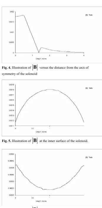
Numerous representations are possible: In Fig. 3 the magnetic filed flux density plot as well the flux lines contour plot are illustrated offering a complete knowledge of the magnetic field. In Fig. 4 the absolute value of versus the distance from the axis of symmetry of the solenoid is illustrated. In Figs. 5 and 6

B

B

is illustrated at the inner and the outer surface of the solenoid (length equal to one inch responds to the axis ). The FEMM software allows a series of other calculations also. For example it gives that the magnetic field energy within the coil is 0.9 times the corresponding value in the air while the total losses in the coil are

W

.

0

z

=

W

334m

=

Fig. 3. Magnetic flux field density representations.

Fig. 4. Illustration of

B

versus the distance from the axis of symmetry of the solenoid

Fig. 5. Illustration of

B

at the inner surface of the solenoid.

Fig. 6. Illustration of

B

at the outer surface of the solenoid.

Example 2: Calculation of the magnetic field and the eddy currents induced in a steel pipe.

A copper wire that runs down the bore of a steel pipe is considered. The wire carries a low–frequency harmonic current

I

=

100e

j2πt

A

( )

. The outer diameter of the pipe is double its inner diameter and ten times the diameter of the copper wire, see Fig. 7. The problem is 2D planar, harmonic LF magnetic. The current in the wire will cause flux to flow along concentric flux paths around the cross– section of the pipe while its time variations induces eddy currents, [21-23], in the pipe, that tend to resist the field created within the wire. The tube is made of steel M19, a non–linear magnetic material with electric conductivity

3 MS m

Fig. 7. Tube with a wire running down its center.

Fig. 8. Proposed model.

The equation to be solved is, [21], the:

(

)

2

2

2 2

d

1 d

1

1

2

d

d

H

H

j

fr

H

r

+

r

r

−

r

+

πμσ

=

0

(15)

where

f

is the current frequency and

μ

and

σ

are respectively the magnetic permeability and conductivity of the medium. The only boundary condition that is used is the at the outer radius of the tube. For increased accuracy and low computational cost different discretization steps (mess sizes) are considered in the different parts of the problem domain, see Fig. 9.

0

=

A

Fig. 9. The discretized problem domain.

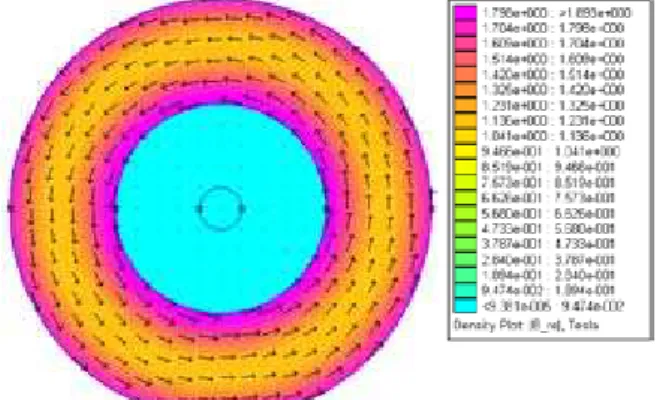
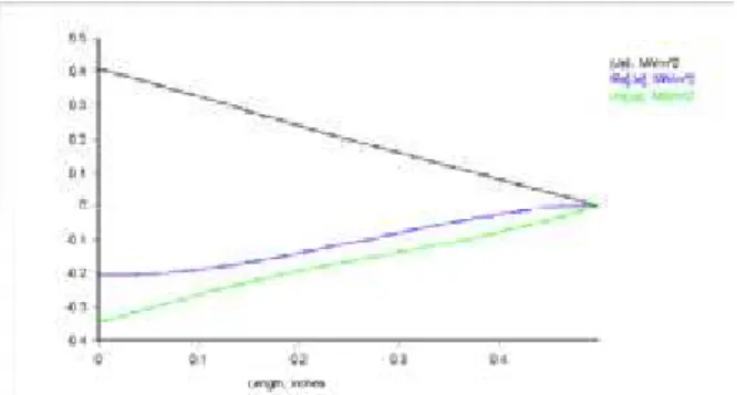
In Figs. 10 and 11 the real and the imaginary parts of the magnetic flux density as well their vector plots are correspondingly illustrated. Results have been found similar to the ones calculated from the theory, [21]. It is noticed that the time dependence of the current flowing through the wire induces eddy currents in the tube with increased values in its inner surface. In Fig. 12 the eddy current density value across the tube radius is depicted ( responds to the inner radius of the tube and to its outer radius). It has to be mentioned that these values are significantly smaller compared to the current that flows through the copper wire. The total energy of the magnetic field is

0

x

=

0.5in

x

=

0.47J

E

=

. In practice this is stored in the steel (99.8% of the total energy).

Fig. 10. Density and vector plot of the real part of the magnetic flux density.

Fig. 12. Illustration of eddy currents induced in the tube.

Example 3: Calculation of the electric field produced by two conducting spheres.

A system of two conducting spheres with diameter at a distance is considered, see Fig. 13. The spheres are set at opposite voltages

and are surrounded by air.

50m

a

=

d

=

70m

1,2

1Volt

V

= ±

d

a

Fig. 13. The system of the two conducting spheres.

The problem is an axisymmetric one. Due to symmetry considerations, only one sphere need be modeled. The line of symmetry between the two spheres is fixed at to account for the effects of the second sphere. In Fig. 14 the proposed model is illustrated.

0Volts

V

=

Fig. 14. Proposed model.

The boundary conditions should be applied are the zero boundary condition to the line of symmetry at

z

=

0

and the mixed BC with

c

₀

=

2

ε ρ

₀ and at the exterior arc of the problem domain, see [17-18] for more details. With

1

c

=

0

0

ε

is denoted the electrical permittivity of the air while

ρ

is the arc radius. The condition is determined from the expression:

2

0

V

V

n

ρ

∂

₊

₌

∂

(16)

where

n

represents the direction normal to the boundary. In Figs. 15 and 16 plots of

Ε

and

V

are respectively presented. From Fig. 16 comes that the field intensity is normal to the surface of the sphere (this can also be verified by designing the tangential electric field intensity across the surface which is significantly smaller compared to the normal field intensity component). The stored energy of the electric field is found

E

=

2.19nJ

and the charge of each sphere is

Q

=

4.45nCb

. From these values system capacity is easily calculated.

Fig. 15. Electric field intensity vector and density plots.

Fig. 16. Electric voltage (electric field scalar potential) density plot and equipotential curves.

5. Conclusions

and engineering. The problems can be solved are 2D planar and 3D axisymmetric ones. The paper provides a brief overview of the software characteristics and its potential applications. A demonstration of its features it presented

through simple examples. Its capability to meet as a complementary tool the needs of science and technology has been shown.

______________________________

References

[1] R. C. Booton Jr, Computational Methods for Electromagnetics and Microwaves, John Wiley & Sons, Inc, New York, (1992). [2] J. L. Volakis, A. Chatterjee., and L. C. Kempel, Finite Element

Methods for Electromagnetics, IEEE Press, USA, (1998). [3] S. Moaveni, Finite Element Analysis: Theory and Application

with ANSYS, 3rd _{ed., Prentice–Hall, Inc., New Jersey, (2007).}

[4] http://femm.foster-miller.net

[5] J. Íñiquez, V. Raposo, A. G. Flores, M. Zazo, and A. Hernández– López, Magnetic levitation by induced eddy currents in non– magnetic conductors and conductivity measurements, Eur. J. Phys., 26, pp. 951-957, (2005).

[6] N. Pamme, Magnetism and microfluidics, Lab Chip, 6, pp. 24-38, (2006).

[7] T. Wichert and H. Kub, Design and optimization of switched reluctance machines, Proc. XLI International Symposium on Electrical Machines (SME 2005), Jarnołtówek, Poland, (2005). [8] O. Rotariu, L. E. Udrea, N. J. C. Strachan, and V. Badesqu,

Targeting magnetic carrier particles in tumor microvasculature – A numerical study, Journal of Optoelectronics and Advanced Materials, 7, pp. 3209-3218, (2005).

[9] Y. S. Lee, G. Kim, V. R. Skoy, and T. Ino, Development of a neutron polarizer 3_{He spin filter at the Pohang neutron facility,}

Journal of the Korean Physical Society, 48, pp. 233-239, (2006). [10] R. Picker, A new superconducting magnetic trap for ultra–cold

neutrons, Diploma thesis, Technische Universität München, Germany, (2004).

[11] C. J. Zandsteeg, Design of a RoboCup Shooting Mechanism, Report 2005.147, Eindhoven University of Technology, The Netherlands, (2005).

[12] M. H. Acuña, B. J. Anderson, C. T. Rusell, P. Wasilewski, G. Kletetshka, L. Zanetti, and N. Omidi, Near magnetic field

observations at 433 Eros: First measurements form the surface of an asteroid, Icarus, 155, pp. 220-228, (2002).

[13] C. Boniface, G. J. M. Hagelaar, L. Garrigues, J. P. Boeuf, and M. Prioul, A Monte–Carlo study of ionization processes in Double Stage Hall Effect Thruster, Proc. XXVIIth ICPIG, topic 19, Eindhoven, The Netherlands, (2005).

[14] K. B. Baltzis, On the usage and potential applications of the finite element method magnetics (FEMM) package in the teaching of electromagnetics in higher education,” in Proc. CBLIS 2007, pp. 408-420, Heraklion, Greece, (2007).

[15] C. A. Balanis, Advanced Engineering Electromagnetics, John Willey & Sons, Inc., New York, (1989).

[16] R. F. Harrington, Time-Harmonic Electromagnetic Fields, IEEE Press, New York, (2001).

[17] D. Meeker, Finite Element Method Magnetics: User’s Manual, 4th

ver., Waltham, (2004)

[18] FEMM 4.0 Electrostatics Tutorial, Waltham, (2004).

[19] N. A. Spaldin, Magnetic Materials: Fundamentals and Device Applications, University Press, Cambridge, (2003).

[20] S. R. Hoole, Computer–aided Analysis and Design of Electromagnetic Devices, Elsevier, New York, (1989)

[21] R. L. Stoll, The Analysis of Eddy Currents, Oxford University Press, Oxford, England, (1974).

[22] A. Krawczyk A. and J. A. Tegopoulos, Numerical Modelling of Eddy Currents, Oxford University Press, USA, (1993).

[23] J. K. Sakellaris, Eddy Currents Modelling in Thin Layers, WSEAS Press, (2007).

[24] R. Ierusalimschy, Programming in Lua, 2nd _{ed., Biblioteca do}