Hydrol. Earth Syst. Sci., 20, 2019–2034, 2016 www.hydrol-earth-syst-sci.net/20/2019/2016/ doi:10.5194/hess-20-2019-2016
© Author(s) 2016. CC Attribution 3.0 License.
Precipitation ensembles conforming to natural variations derived
from a regional climate model using a new bias correction scheme
Kue Bum Kim1, Hyun-Han Kwon2, and Dawei Han1
1Water and Environmental Management Research Centre, Department of Civil Engineering, University of Bristol, Bristol, UK 2Department of Civil Engineering, Chonbuk National University, Jeonju-si, Jeollabuk-do, South Korea
Correspondence to:Hyun-Han Kwon ([email protected])
Received: 20 August 2015 – Published in Hydrol. Earth Syst. Sci. Discuss.: 9 October 2015 Revised: 15 April 2016 – Accepted: 29 April 2016 – Published: 17 May 2016
Abstract.This study presents a novel bias correction scheme for regional climate model (RCM) precipitation ensembles. A primary advantage of using model ensembles for climate change impact studies is that the uncertainties associated with the systematic error can be quantified through the en-semble spread. Currently, however, most of the conventional bias correction methods adjust all the ensemble members to one reference observation. As a result, the ensemble spread is degraded during bias correction. Since the observation is only one case of many possible realizations due to the cli-mate natural variability, a successful bias correction scheme should preserve the ensemble spread within the bounds of its natural variability (i.e. sampling uncertainty). To demon-strate a new bias correction scheme conforming to RCM pre-cipitation ensembles, an application to the Thorverton catch-ment in the south-west of England is presented. For the en-semble, 11 members from the Hadley Centre Regional Cli-mate Model (HadRM3-PPE) data are used and monthly bias correction has been done for the baseline time period from 1961 to 1990. In the typical conventional method, monthly mean precipitation of each of the ensemble members is nearly identical to the observation, i.e. the ensemble spread is removed. In contrast, the proposed method corrects the bias while maintaining the ensemble spread within the nat-ural variability of the observations.
1 Introduction
The growing evidence of global climate change is clear in the past century (Stocker, 2013). Therefore, future projections of climate that incorporate the effects of an underlying
chang-ing climate are of great importance, particularly because of reliance of mitigation and adaptation on realistic projections. Interest in the impacts of climate change is increasing from water resources managers in the context of the hydrological cycle and water resources (Bates et al., 2008; Arnell et al., 2001). Global climate models (GCMs) are usually used for the projection of future climate and the accuracy of GCMs has been enhanced in simulating large-scale global climate. Nevertheless, GCMs have difficulties in providing reliable climate data at local scales due to their coarse resolutions (100–250 km) (Maraun et al., 2010). Therefore, for regional impact studies, regional climate models (RCMs) have been widely used which are compatible with the catchment scales (25–50 km).
there are relatively too many low-intensity wet days com-pared with the observations (Ehret et al., 2012; Ines and Hansen, 2006).
The errors along with the mismatching scales have re-sulted in numerous studies on developing and evaluating the bias correction methods (Chen et al., 2011a, b; Johnson and Sharma, 2011; Piani et al., 2010; Teutschbein and Seib-ert, 2012). Evaluation of different bias correction methods has been done by Teutschbein and Seibert (2012): (1) linear scaling (Lenderink et al., 2007), (2) local intensity scaling (Schmidli et al., 2006), (3) power transformation (Leander and Buishand, 2007; Leander et al., 2008), and (4) the dis-tribution mapping method (Block et al., 2009; Déqué et al., 2007; Johnson and Sharma, 2011; Piani et al., 2010; Sun et al., 2011). The linear scaling method adjusts the mean value of the model to that of the observation by applying a cor-rection factor which is the ratio between the long-term ob-servation and model data. However, the local intensity scal-ing method considers wet-day frequency and wet-day inten-sity as well as the bias in the mean. The power transfor-mation method corrects the mean and variance of the data. The distribution mapping method fits the distribution func-tion of the climate model data to that of the observafunc-tion. The results have shown that all four bias correction meth-ods could improve the raw RCM precipitation. Among them, the distribution mapping method is the best; however, it has the drawback of overfitting. Although the bias correction is commonly applied in climate change studies, correcting the model output towards the corresponding observation is still a controversial issue, and applying bias correction could make the uncertainty range of the simulations narrower, i.e. “hides rather than reduces uncertainty” (Ehret et al., 2012).
In this study we address the issue which most conven-tional bias correction methods implicitly neglect: the uncer-tainty associated with the observation sampling unceruncer-tainty. We note that adjusting the statistical properties of each of the ensemble members to one observation does not preserve the spread across the ensemble members, thus negating the advantage of quantifying uncertainty through the use of en-semble spread in climate change impact studies. In general, uncertainties in climate change projections can be grouped by three main sources: boundary condition, model structure, and natural variability (Hawkins and Sutton, 2009). To ac-count for these sources of uncertainties, ensemble modelling is a generally accepted way of producing a number of sim-ulations using multiple scenarios, different models (struc-tures and parameters), and initial conditions (Collins et al., 2006; Good and Lowe, 2006; Meehl et al., 2005; Murphy et al., 2004; Palmer and Räisänen, 2002; Stainforth et al., 2005; Tebaldi et al., 2006; Webb et al., 2006; Weisheimer and Palmer, 2005) which are possible due to an increase in data availability through high-performance computing sys-tems. There are two approaches for ensemble schemes in the context of model uncertainty. The first is the multi-model ensemble (MME) method to address the structural
uncer-tainty associated with the understanding and parameteriza-tion of the GCMs which is applied in the Intergovernmen-tal Panel on Climate Change (IPCC) assessments (Meehl et al., 2007; Solomon, 2007; Taylor et al., 2012). The second is the perturbed-physics ensemble (PPE) method which is gen-erated by perturbing physical parameters in a given climate model and is complementary to the MME approach.
K. B. Kim et al.: Precipitation ensembles conforming to natural variations 2021
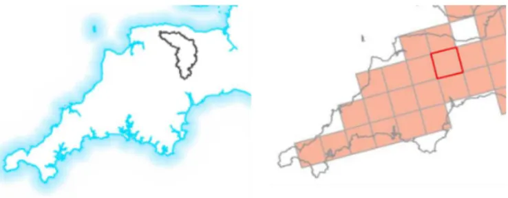
Figure 1.Location of the Thorverton catchment (the left panel) and HadRM3 25 km grid boxes (the right panel). The highlighted grid box in red is selected to cover the Thorverton catchment.
There are many aspects (e.g. mean, variance, skewness, autocorrelation) of the rainfall series which cannot be all cor-rected simultaneously. The way of correcting the RCM data should therefore depend on what properties are relevant to the data usage. In this study we have focused on the use of the spread of bias corrected RCM precipitation to investigate the impact of the conventional and proposed bias correction schemes on the flow. The conventional method removes the spread of the ensemble, while the proposed method can bet-ter convey the spread properties of the ensemble.
The paper is structured as follows: Sect. 2 describes the study catchment and data; in Sect. 3 the conventional bias correction method is presented. Next we show how the ob-servation sampling uncertainty (i.e. natural variability) is es-timated and how the ensemble is evaluated. Finally the con-cepts of conventional and proposed bias correction methods are compared. In Sect. 4 we show the results followed by a discussion and conclusions in Sects. 5 and 6.
2 Catchment and data
The Thorverton catchment is used as the case study site. It has an area of 606 km2, and is a sub-catchment of the Exe catchment. The Exe catchment is located in the south-west of England, with an area of 1530 km2and an average annual rainfall of 1088 mm. Figure 1 shows the overview of the Exe catchment area. Daily time series of the observed precipi-tation data (1961–1990) over the Thorverton catchment are obtained from the UK Met Office.
The climate data used in this study are the Hadley Centre Regional Climate Model (HadRM3-PPE) data which were generated by the Met Office Hadley Centre. This data set is used to dynamically downscale regional projections of the future climate from the HadCM3 GCM (Murphy et al., 2009). It is comprised of 11 members (1 unperturbed and 10 perturbed members). For the perturbation, 31 parameters are chosen from the unperturbed member representing radiation, land surface, boundary layer, sea ice, cloud, atmospheric dy-namics, and convection (Collins et al., 2011). The data set provides the time series of climate data in the period 1950– 2100 for the A1B historical and future medium emission
sce-nario. The temporal and spatial resolutions of the HadRM3 climate data are daily and 25 km (0.22◦ on a rotated pole
grid) respectively. Here, the daily precipitation series from all 11 members are used to evaluate the ensemble and to test the proposed new bias correction scheme for the baseline pe-riod of 1961 to 1990. The grid is chosen to cover the study catchment.
3 Methodology
3.1 Conventional bias correction method
Bias correction was initially proposed for calibrating the sea-sonal GCM variables (e.g. precipitation and temperature) and later extended to the daily timescale. Individual months are usually processed independently of each other, in order to correct seasonal phase errors, after modifying the wet-day frequency of the climate model precipitation on the wet-day observed frequency by applying a cut-off threshold. Com-pared with the observations, the climate model precipitations usually have more wet days at low precipitation. In this study the two-parameter Gamma distribution is used to fit the ob-served precipitation:
f (x)= 1 βαŴ (α)x
α−1e−x/β;x≥
0;αβ >0, (1) whereŴis the gamma function andαandβ are the shape and scale parameters respectively.
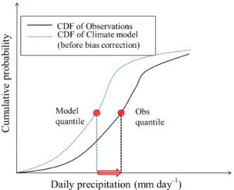
Figure 2.A schematic representation of the concept of the conven-tional quantile mapping method for bias correction.
scale parameter. The subscripts model and obs indicate the parameters from the RCM and observed precipitation.
In this study, daily bias correction is applied for each month separately. December, which is a wet period in the study catchment, is used to illustrate the new bias correction method in more detail.
3.2 Natural variability of observation
The problem with the conventional bias correction methods is that all the ensemble members are adjusted to one obser-vation as a reference value. As a result, the spread of the en-semble which represents the uncertainty is removed after bias correction. However, due to the observational sampling un-certainty in terms of climate variability, the observation is only one case of many possible realizations. Climate natural variability is a natural fluctuation that occurs without external forcing to the climate system. To estimate the natural vari-ability of the observed precipitation, the parameters of the Gamma distribution for December daily precipitation from 1961 to 1990 are assumed to be the true parameters. We use 100 000 sets of 30-year daily precipitation random samples from the true parameters. For each sample (i.e. 30-year daily rainfall simulation), we estimate a set of new Gamma param-eters (i.e. shape and scale parameter). The re-estimated pa-rameters are different to those used in the simulations due to the observation sampling uncertainty. In this study, the distri-bution of 100 000 sets of parameters is assumed to represent the natural variability of 30-year daily precipitation. In order to find the optimized number of resampling, the sensitivity analysis between the numbers of resampling and the mean value of the observed precipitation has been done. The result has shown that beyond 20 000 resamples, the mean value be-comes stable. Since the running time does not take long in this study, we have resampled 100 000 times, which are suf-ficient.
3.3 Evaluation of ensemble members
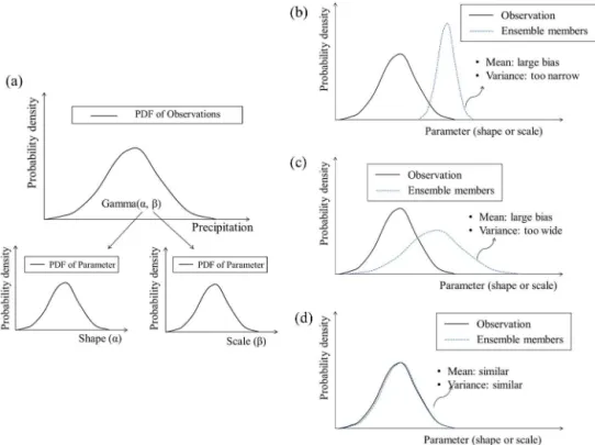
The ensemble members must first be evaluated to assess whether bias correction is necessary. The idea of evaluating the ensemble members is illustrated in Fig. 3. The observed daily precipitation is assumed to follow the Gamma distri-bution defined by the shape and scale parameters. The dis-tribution of the parameters can be derived from the resam-pling procedure as mentioned in Sect. 3.2 (Fig. 3a). Then we compare the distributions of the observation and ensemble members’ parameters (Fig. 3b–c). If the parameter distribu-tion of an ensemble member looks like Fig. 3b, the mem-ber has bias in mean and variance (in the form of a shifted and narrow parameter distribution). If the parameter distri-butions were biased on the mean and had a wide variance, it resembles something closer to Fig. 3c. Both of these “cases” indicate the need for bias correction. On the other hand, if the parameter distribution of an ensemble member resem-bles Fig. 3d (i.e. similar mean and variance of the ensem-ble member and empirical estimate), then bias correction is not necessary. The basic idea of the proposed bias correction is to match the shapes of parameter distribution between the observation and ensemble members so that they are similar after bias correction rather than matching point estimates of the parameters.
3.4 Comparison between the conventional and proposed bias correction schemes
K. B. Kim et al.: Precipitation ensembles conforming to natural variations 2023
Figure 3.A schematic representation of the evaluation of ensemble members.
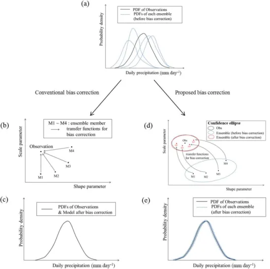
of 11 members are reasonably well corrected without elimi-nating the spread of the ensemble (Fig. 4e).
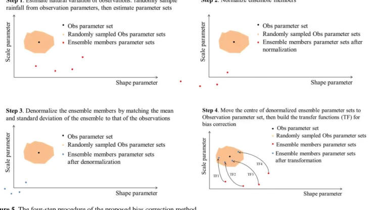
A step by step summary of the proposed procedure is pre-sented as follows and in Fig. 5.
(Step 1) Natural variability of the observation is estimated by first randomly resampling precipitation from a Gamma distribution with parameters obtained by fitting the observed precipitation. Next, the parameters of each resampled precip-itation time series are estimated, and the bivariate distribution of these parameters over all the samples is established. The shaded area in Fig. 5 represents the natural variability of the observation. If the parameters of the ensemble members are in the shaded area, there is no need to do bias correction.
(Step 2) Normalize the parameters of the ensemble mem-bers using Eq. (3).
xN= x−µx
σx
, yN= y−µy
σy
, (3)
wherexandy are the shape and scale parameters of the dis-tribution of each ensemble member,µx, µyare the mean val-ues,σx, σyare the standard deviations of the parameters of all ensemble members, andxNandyNare the normalized shape and scale parameters.
(Step 3) De-normalize the parameters of the ensemble members by matching the mean and standard deviation to those of the observation as shown in Eq. (4).
x′=xN·σxo+µxo , y′=yN·σyo+µyo, (4)
whereµxo, µyoare the mean values andσxo, σyoare the stan-dard deviations of the parameters of the observation;x′,y′ are the de-normalized shape and scale parameters.
(Step 4) In Step 3, the coordinate of the centre of the de-normalized ensemble parameter sets is (0, 0). This coordi-nate is shifted to that of the observation (i.e. the black dot in Fig. 5, Step 4), which results in the ensemble members’ pa-rameter sets falling into the boundary of the natural variation of the observations. From this, transfer functions for the bias correction can be built.
3.5 Hydrological application
To investigate the impact of different bias correction schemes on flow, we have used a conceptual rainfall–runoff model called IHACRES (Jakeman and Hornberger, 1993). This model has been widely applied to a variety of catchments for hydrological analysis and climate impact studies (Jake-man et al., 1993; Kim and Lee, 2014; Letcher et al., 2001; Littlewood, 2002). The model is composed of a non-linear module and a linear module as shown in Fig. 6. The details of this model are described in Appendix A.
Figure 4.A schematic representation of the conventional bias correction method and the proposed bias correction method.
the IHACRES model. Third, the optimized parameters and the ensemble of precipitation forcings are then used to simu-late daily flow ensembles. Finally, from these daily simusimu-lated flow data, 30-year mean monthly flow has been estimated and compared for the two different bias correction schemes.
4 Results
The first part of this section compares the parameter dis-tribution of the observed precipitation and bias uncorrected precipitation. The next part shows the result of the conven-tional bias correction followed by the proposed bias correc-tion method. In each part, PDFs of precipitacorrec-tion, shape, and scale parameter space and PDFs of shape and scale parame-ters have been evaluated and compared. Finally, the monthly mean precipitation for the time period from 1961 to 1990 is compared among the observation, uncorrected ensemble members, and corrected ensemble members by applying both the conventional and new methods.
4.1 Parameter distribution of the observed and RCM precipitation
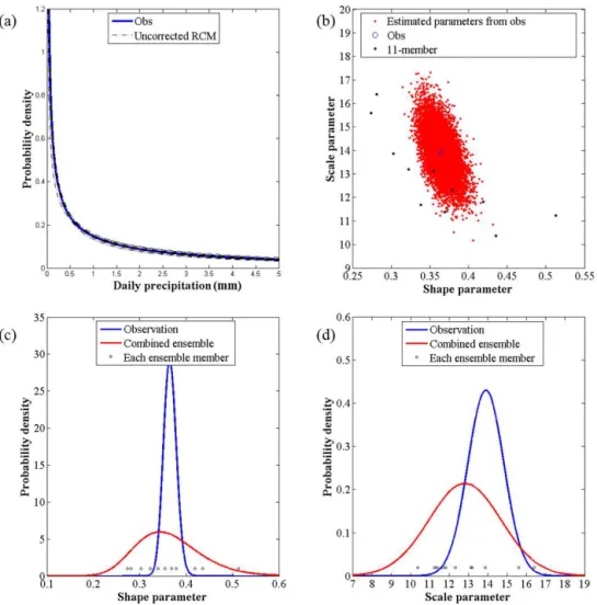
Before correcting the bias of each member, we compare the statistical properties with the observed precipitation. Fig-ure 7a shows the PDFs of the observed and simulated pre-cipitation. The parameter space (i.e. shape vs. scale parame-ter) of these distributions is plotted in Fig. 7b as illustrated in Sect. 3.2. The red dots represent the natural variability of the observation which is estimated from the observed pa-rameters. Most of the members’ parameters are outside the boundary of the natural variability. Figure 7c and d compare the distribution of each parameter. The distribution of the pa-rameter for the combined ensemble shows large biases of the mean and variance. Since both the mean and variance of the 11 members are quite different to those of the observation, it is apparent that bias correction is needed.
K. B. Kim et al.: Precipitation ensembles conforming to natural variations 2025
Figure 5.The four-step procedure of the proposed bias correction method.
Figure 6.Structure of the IHACRES model.
variability of monthly mean precipitation which has been es-timated from the resampled precipitation.
4.2 Conventional bias correction
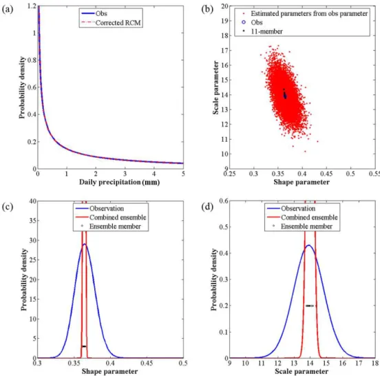
Figure 9 illustrates the result of the conventional bias cor-rection method. As expected, the PDFs of the observation and 11-member ensemble are nearly identical to one another (Fig. 9a), and the parameters of the corrected precipitation are all in the centre of the parameter space of the observation (Fig. 9b, c, and d). As previously noted, the spread of the en-semble under this conventional approach is greatly reduced, and, in turn, the overall characteristics of hydro-climate vari-ables are nearly identical across different model runs.
4.3 Proposed bias correction
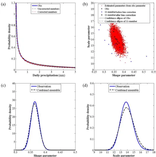
To preserve the spread of the ensemble members, a system-atic modelling scheme is proposed. Figure 10a presents the PDFs of the observation, bias uncorrected members, and bias corrected members. One can see that the corrected members, although they are not exactly the same as the observation, are closer to the observation than the uncorrected members. It is clearer if we see the result in terms of the parameter space (Fig. 10b). The parameters of the corrected members are all within the boundary of the natural variability of the observed precipitation. In addition, the distributions of the 11 members’ parameters after bias correction are quite sim-ilar to those of the observation (Fig. 10c and d). Therefore, one can assume that all ensemble members represent realistic precipitation scenarios when the natural variability is consid-ered.
4.4 Comparison of bias corrected monthly mean precipitation
Figure 7. Parameter distributions of the observation and 11 members:(a)probability density function of the observed and 11-member precipitation time series before bias correction;(b)scatter plot between shape and scale parameters of the observed and bias uncorrected precipitation;(c–d)probability density functions of shape and scale parameters for the observed and bias uncorrected precipitation.
Figure 8. (a)PDFs of the observed precipitation and the resampled precipitation;(b)natural variability of monthly mean precipitation.
method, the corrected monthly mean precipitation of all 11 members is very similar to the observation, and the spread of the ensemble is almost entirely removed (Fig. 11b). Correc-tion through the proposed method results in simulated
K. B. Kim et al.: Precipitation ensembles conforming to natural variations 2027
Figure 9.Results of the conventional bias correction method:(a)probability density functions of the observed and simulated (i.e. 11-member) precipitation after bias correction;(b)scatter plot between shape and scale parameters of the observed and bias corrected precipitation;(c–d)
probability density functions of the shape and scale parameters of the observed and bias corrected precipitation.
4.5 Hydrological application
As presented in Fig. 11, the bias and spread of monthly mean precipitation using the proposed bias correction method are more variable than the conventional method. Next, to investi-gate the impact of these two different bias correction schemes on flow simulations, we used the aforementioned hydrologi-cal model (IHACRES). Since the focus of the proposed bias correction scheme is on correcting the mean value and the spread of RCM precipitation ensembles, the same character-istics have been examined in the simulated flow.
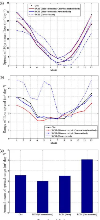
Figure 12a shows the range of monthly mean flow simu-lated from the precipitation ensembles for the period 1961– 1990. The 5–95th percentile spread has been plotted. Fig-ure 12b shows the range of monthly spread, i.e. the differ-ence between the two lines in Panel (a). Figure 12c shows the annual average value of the range, i.e. the mean value of each line in Panel (b). The flow ensemble simulated from the
Figure 10.Results of the proposed bias correction method:(a)probability density functions of the observed, bias uncorrected, and bias corrected precipitation;(b)scatter plot between the shape and scale parameters of the observed, bias uncorrected, and bias corrected precip-itation;(c–d)probability density functions of the shape and scale parameters of the observed and bias corrected precipitation.
Figure 11.Monthly mean precipitation for the period 1961–1990 derived from the model simulations. The mean values for the observation and 11 members are displayed as well.(a)Uncorrected 11 members;(b)corrected 11 members by the conventional bias correction; and
K. B. Kim et al.: Precipitation ensembles conforming to natural variations 2029
Figure 12. (a) The range of monthly mean flow simulated from the precipitation ensembles for the period 1961–1990 (5–95th per-centile spread);(b)the range of monthly spread;(c)annual average value of the range.
4.6 One transfer function for 11 members
An experiment is carried out to identify whether to correct each member individually or to treat them as a group. The idea is that in order to maintain the spread of 11 members, in-stead of using each transfer function for an individual ber, only one transfer function from the unperturbed mem-ber is built based on the conventional method, and then this transfer function is applied to the rest of the members. If only
one transfer function is used for correcting the biases of 11 members, those members may maintain the spread after bias correction. However, if the spread is not properly preserved, the corrected ensemble will not represent the true variation of 11 members. Figure 13 shows an example of using one transfer function. The transfer function is built by matching the CDF of an unperturbed member to that of the observation and this transfer function is applied to the other 10 members. As shown in the figure, the spread of the 11-member param-eters after bias correction is not matched by the spread of the observation. Therefore, the existing approach based on the conventional bias correction scheme generally fails to pre-serve the ensemble spread. However, on the other hand, the result of applying one transfer function can also be a possible realization depending on how to estimate the natural variabil-ity of the observation which is discussed in the next section.
5 Discussion
Climate change scenarios are generated using climate mod-els (e.g. GCMs and RCMs) and emission scenarios, and are the key information for understanding future changes in hy-drologic systems. While RCMs are designed to better simu-late local climate at finer spatial and temporal scales, it has been acknowledged that bias correction for the outputs from RCMs is generally required to reduce biases due to system-atic errors. An ensemble approach has previously been in-troduced to deal with the systematic errors (i.e. uncertain-ties) and to provide more relevant scenarios informed by a probability density function. However, the spread of the en-semble, with useful information to understand uncertainties, has not been properly considered in the existing bias correc-tion scheme. In other words, all the ensemble members are matched to the observations in terms of statistical character-istics, so that the advantage of the ensemble with respect to a single model output is excluded. The major contribution of this study is the proposal of a new bias correction scheme, which reasonably preserves the spread of the RCM ensemble members.
Figure 13.Result of using one transfer function for bias correction.
member rather than pooling all the members in the bias cor-rection procedure.
Ideally, if we have numerous numbers of observation data, more reliable climate statistics could be derived. However, in reality, 30 years of observation data have been used as the reference climate, which is just one realization of many pos-sibilities, and the uncertainty associated with distributional parametric uncertainty needs to be considered in designing and conducting impact studies of climate change. Distribu-tional parametric uncertainty exists when limited amounts of hydrologic data are used to estimate the parameters of PDFs. On the other hand, initial conditions or parameters in climate models can be perturbed to generate a large number of en-semble members. Given the results we achieve, these ensem-ble members need to be examined to ensure that they are plausible.
This study attempts to evaluate the reliability of the RCM ensemble in terms of natural variability and to propose a new bias correction scheme conforming to the RCM ensembles. However, the proposed scheme is just one of the necessary conditions to assess the RCM ensembles, and a comprehen-sive scheme including more conditions, if any, needs to be further developed. It does not mean that the RCM which meets this condition is a good model, but if it does not meet this condition, the RCM ensemble fails to represent the nat-ural climate variation (hence such a condition is a necessary condition, not a sufficient condition). We believe that there should be a set of necessity conditions to better assess and improve future climate projections in various aspects of un-certainty analysis.
We would like to point out some limitations of this study. First, as previously mentioned, bias correction is a contro-versial issue. In addition, there are no generic one-suit-fits-all bias correction methods for rainfone-suit-fits-all data, since rainfone-suit-fits-all time series have many aspects and cannot be all corrected si-multaneously. The way of correcting the bias should depend on the data purpose, since the bias depends on the specific rainfall characteristic (Kew et al., 2011). In this study, we
K. B. Kim et al.: Precipitation ensembles conforming to natural variations 2031 6 Conclusions
Conventionally, all climate model simulations are corrected to the observation. With this scheme, the uncertainty of the model from the ensembles will be lost and as a result the 11-member ensemble will be similar to just 1 11-member. Another approach is to apply one transfer function based on the unper-turbed member to the remaining 10 members. This will keep the spread properties of the ensemble, but this spread may not conform to the spread from the real natural system. Therefore they do not look as if they are drawn from the natural system. In this study, we have proposed a new scheme which over-comes the shortcomings of the aforementioned two schemes (i.e. 11 transfer functions all conformed to one observed alization or 1 transfer function for 11 members, which re-sults in the bias corrected ensembles being too narrow or too
Appendix A: Hydrological model IHACRES
The IHACRES model is composed of a non-linear module and a linear module as shown in Fig. 6 and the model param-eters are listed in Table A1. A non-linear module converts total rainfall to effective rainfall, which is calculated from Eq. (A1).
Uk=[C (k−l)]prk, (A1) whererk is the observed rainfall,C is the mass balance,lis the soil moisture index threshold, andpis the power on soil moisture respectively. The soil moisture (∅k)is calculated from
∅k=rk+(1− 1 τk
)∅k−1, (A2) whereτkis the drying rate given by
τk=τwexp[0.062f (tr−tk)], (A3) whereτwis the drying rate at the reference temperature,f is the temperature modulation,tris the reference temperature, andtkis the observed temperature. A linear module assumes that there is a linear relationship between the effective rain-fall and flow. Two components in this module, quick flow and slow flow, can be connected in parallel or in series. In this study two parallel storages in the linear module are used because such a combination reflects the catchment conditions and the streamflow (xk)at time stepkis defined by the fol-lowing equations:
xk=x( q) k +x
(s)
k , (A4)
xk(q)=βqUk−αqxk(q−)1, (A5) xk(s)=βsUk−αsxk(s−)1, (A6) wherex(kq)andxk(s)are quick flow and slow flow respectively, and α andβ are recession rate and peak response respec-tively. The relative volumes of quick flow and slow flow can be calculated from
Vq=1−Vs= βq 1+αq
=1− βs 1+αs
. (A7)
Table A1.Parameters in the IHACRES model. Module Parameter Description
Non-linear c Mass balance
τw Reference drying rate
f Temperature modulation of
drying rate
Linear αq, αs, Quick and slow flow recession rate
βq, βs Fractions of effective rainfall for peak response
τs Slow flow recession time con-stant,τs= −1/ln(−αs) τq Quick flow recession time
K. B. Kim et al.: Precipitation ensembles conforming to natural variations 2033 Acknowledgements. The first author is grateful for the financial
support from the Government of the Republic of Korea for carrying out his PhD study at the University of Bristol. The second author was supported by a grant (13SCIPA01) from the Smart Civil Infrastructure Research Program funded by the Ministry of Land, Infrastructure and Transport (MOLIT) of the Korean Government and the Korea Agency for Infrastructure Technology Advancement (KAIA). Finally, we are grateful to editor Bart van den Hurk, reviewer Christiana S. Photiadou, and an anonymous reviewer for their valuable comments and suggestions on the manuscript. The data used in this study are available upon request from the corresponding author via email ([email protected]).
Edited by: B. van den Hurk
References
Addor, N. and Fischer, E. M.: The influence of natural vari-ability and interpolation errors on bias characterization in RCM simulations, J. Geophys. Res.-Atmos., 120, 10180–10195, doi:doi:10.1002/2014JD022824, 2015.
Arnell, N. W., Liu, C., Compagnucci, R. da Cunha, L., Hanaki, K., Howe, C., Mailu, G., Shiklomanov, I., and Stakhiv, E.: Hy-drology and water resources, in: Climate Change 2001: Impacts, Adaptation and Vulnerability. Contribution of Working Group II to the Third Assessment Report of the Intergovernmental Panel on Climate Change, edited by: McCarthy, J. J., Canziani, O. F., Leary, N. A., Dokken, D. J., and White, K. S., Cambridge Uni-versity Press, Cambridge, 191–233, 2001.
Baigorria, G. A., Jones, J. W., Shin, D.-W., Mishra, A., and O’Brien, J. J.: Assessing uncertainties in crop model simulations using daily bias-corrected Regional Circulation Model outputs, Clim. Res., 34, 211–222, doi:10.3354/cr00703, 2007.
Bates, B., Kundzewicz, Z. W., Wu, S., and Palutikof, J.: Climate change and water, Intergovernmental Panel on Climate Change (IPCC), 2008.
Block, P. J., Souza Filho, F. A., Sun, L., and Kwon, H. H.: A Stream-flow Forecasting Framework using Multiple Climate and Hy-drological Models1, J. Am. Water Resour. Assoc., 45, 828–843, 2009.
Bromwich, D. H., Otieno, F. O., Hines, K. M., Manning, K. W., and Shilo, E.: Comprehensive evaluation of polar weather research and forecasting model performance in the Antarctic, J. Geophys. Res.-Atmos., 118, 274–292, 2013.
Chen, J., Brissette, F. P., and Leconte, R.: Uncertainty of downscal-ing method in quantifydownscal-ing the impact of climate change on hy-drology, J. Hydrol., 401, 190–202, 2011a.
Chen, J., Brissette, F. P., Poulin, A., and Leconte, R.: Overall un-certainty study of the hydrological impacts of climate change for a Canadian watershed, Water Resour. Res., 47, W12509, doi:10.1029/2011WR01060, 2011b.
Chen, J., Brissette, F. P., Chaumont, D., and Braun, M.: Finding appropriate bias correction methods in downscaling precipitation for hydrologic impact studies over North America, Water Resour. Res., 49, 4187–4205, 2013.
Collins, M., Booth, B. B., Harris, G. R., Murphy, J. M., Sexton, D. M., and Webb, M. J.: Towards quantifying uncertainty in tran-sient climate change, Clim. Dynam., 27, 127–147, 2006.
Collins, M., Booth, B. B., Bhaskaran, B., Harris, G. R., Murphy, J. M., Sexton, D. M., and Webb, M. J.: Climate model errors, feedbacks and forcings: a comparison of perturbed physics and multi-model ensembles, Clim. Dynam., 36, 1737–1766, 2011. Dee, D., Källén, E., Simmons, A., and Haimberger, L.: Comments
on “Reanalyses suitable for characterizing long-term trends”, B. Am. Meteorol. Soc., 92, 65–70, 2011.
Déqué, M., Rowell, D., Lüthi, D., Giorgi, F., Christensen, J., Rockel, B., Jacob, D., Kjellström, E., De Castro, M., and van den Hurk, B.: An intercomparison of regional climate simula-tions for Europe: assessing uncertainties in model projecsimula-tions, Climatic Change, 81, 53–70, 2007.
Ehret, U., Zehe, E., Wulfmeyer, V., Warrach-Sagi, K., and Liebert, J.: HESS Opinions “Should we apply bias correction to global and regional climate model data?”, Hydrol. Earth Syst. Sci., 16, 3391–3404, doi:10.5194/hess-16-3391-2012, 2012.
Feddersen, H. and Andersen, U.: A method for statistical down-scaling of seasonal ensemble predictions, Tellus A, 57, 398–408, 2005.
Good, P. and Lowe, J.: Emergent behavior and uncertainty in multi-model climate projections of precipitation trends at small spatial scales, J. Climate, 19, 5554–5569, 2006.
Hawkins, E. and Sutton, R.: The potential to narrow uncertainty in regional climate predictions, B. Am. Meteorol. Soc., 90, 1095– 1107, 2009.
Ines, A. V. and Hansen, J. W.: Bias correction of daily GCM rainfall for crop simulation studies, Agr. Forest Meteorol., 138, 44–53, 2006.
Jakeman, A. and Hornberger, G.: How much complexity is war-ranted in a rainfall-runoff model?, Water Resour. Res., 29, 2637– 2649, 1993.
Jakeman, A., Littlewood, I., and Whitehead, P.: An assessment of the dynamic response characteristics of streamflow in the Balquhidder catchments, J. Hydrol., 145, 337–355, 1993. Johnson, F. and Sharma, A.: Accounting for interannual
vari-ability: A comparison of options for water resources climate change impact assessments, Water Resour. Res., 47, W04508, doi:10.1029/2010WR009272, 2011.
Jones, P., Kilsby, C., Harpham, C., Glenis, V., and Burton, A.: UK Climate Projections science report: Projections of future daily climate for the UK from the Weather Generator, University of Newcastle, UK, 2009.
Kew, S. F., Selten, F. M., Lenderink, G., and Hazeleger, W.: Robust assessment of future changes in extreme precipitation over the Rhine basin using a GCM, Hydrol. Earth Syst. Sci., 15, 1157– 1166, doi:10.5194/hess-15-1157-2011, 2011.
Kim, H. and Lee, S.: Assessment of a seasonal calibration technique using multiple objectives in rainfall–runoff analysis, Hydrol. Pro-cess., 28, 2159–2173, 2014.
Kotlarski, S., Block, A., Böhm, U., Jacob, D., Keuler, K., Knoche, R., Rechid, D., and Walter, A.: Regional climate model simu-lations as input for hydrological applications: evaluation of un-certainties, Adv. Geosci., 5, 119–125, doi:10.5194/adgeo-5-119-2005, 2005.
Leander, R. and Buishand, T. A.: Resampling of regional climate model output for the simulation of extreme river flows, J. Hy-drol., 332, 487–496, 2007.
re-sampling of regional climate model output, J. Hydrol., 351, 331– 343, 2008.
Lenderink, G., Buishand, A., and van Deursen, W.: Estimates of future discharges of the river Rhine using two scenario method-ologies: direct versus delta approach, Hydrol. Earth Syst. Sci., 11, 1145–1159, doi:10.5194/hess-11-1145-2007, 2007. Letcher, R., Schreider, S. Y., Jakeman, A., Neal, B., and Nathan, R.:
Methods for the analysis of trends in streamflow response due to changes in catchment condition, Environmetrics, 12, 613-630, 2001.
Littlewood, I. G.: Improved unit hydrograph characterisation of the daily flow regime (including low flows) for the River Teifi, Wales: towards better rainfall-streamflow models for regionali-sation, Hydrol. Earth Syst. Sci., 6, 899–911, doi:10.5194/hess-6-899-2002, 2002.
Maraun, D., Wetterhall, F., Ireson, A., Chandler, R., Kendon, E., Widmann, M., Brienen, S., Rust, H., Sauter, T., and The-meßl, M.: Precipitation downscaling under climate change: Recent developments to bridge the gap between dynami-cal models and the end user, Rev. Geophys., 48, RG3003, doi:10.1029/2009RG000314, 2010.
Meehl, G. A., Arblaster, J. M., and Tebaldi, C.: Understand-ing future patterns of increased precipitation intensity in cli-mate model simulations, Geophys. Res. Lett., 32, L18719, doi:10.1029/2005GL023680, 2005.
Meehl, G. A., Covey, C., Taylor, K. E., Delworth, T., Stouffer, R. J., Latif, M., McAvaney, B., and Mitchell, J. F.: The WCRP CMIP3 multimodel dataset: A new era in climate change research, B. Am. Meteorol. Soc., 88, 1383–1394, 2007.
Murphy, J., Sexton, D., Jenkins, G., Boorman, P., Booth, B., Brown, K., Clark, R., Collins, M., Harris, G., and Kendon, E.: UKCP09 Climate change projections, Met Office Hadley Centre, Exeter, 2009.
Murphy, J. M., Sexton, D. M., Barnett, D. N., Jones, G. S., Webb, M. J., Collins, M., and Stainforth, D. A.: Quantification of modelling uncertainties in a large ensemble of climate change simulations, Nature, 430, 768–772, 2004.
Palmer, T. and Räisänen, J.: Quantifying the risk of extreme sea-sonal precipitation events in a changing climate, Nature, 415, 512–514, 2002.
Piani, C., Haerter, J., and Coppola, E.: Statistical bias correction for daily precipitation in regional climate models over Europe, Theor. Appl. Climatol., 99, 187–192, 2010.
Schmidli, J., Frei, C., and Vidale, P. L.: Downscaling from GCM precipitation: a benchmark for dynamical and statistical down-scaling methods, Int. J. Climatol., 26, 679–689, 2006.
Solomon, S.: Climate change 2007-the physical science basis: Working group I contribution to the fourth assessment report of the IPCC, Cambridge University Press, 2007.
Stainforth, D. A., Aina, T., Christensen, C., Collins, M., Faull, N., Frame, D., Kettleborough, J., Knight, S., Martin, A., and Murphy, J.: Uncertainty in predictions of the climate response to rising levels of greenhouse gases, Nature, 433, 403–406, 2005. Stocker, D. Q.: Climate change 2013: The physical science basis,
Working Group I Contribution to the Fifth Assessment Report of the Intergovernmental Panel on Climate Change, Summary for Policymakers, IPCC, 2013.
Sun, F., Roderick, M. L., Lim, W. H., and Farquhar, G. D.: Hy-droclimatic projections for the Murray-Darling Basin based on an ensemble derived from Intergovernmental Panel on Climate Change AR4 climate models, Water Resour. Res., 47, W00G02, doi:10.1029/2010WR009829, 2011.
Taylor, K. E., Stouffer, R. J., and Meehl, G. A.: An overview of CMIP5 and the experiment design, B. Am. Meteorol. Soc., 93, 485–498, 2012.
Tebaldi, C., Hayhoe, K., Arblaster, J. M., and Meehl, G. A.: Going to the extremes, Climatic Change, 79, 185–211, 2006.
Teutschbein, C. and Seibert, J.: Bias correction of regional climate model simulations for hydrological climate-change impact stud-ies: Review and evaluation of different methods, J. Hydrol., 456, 12–29, 2012.
Thorne, P. and Vose, R.: Reanalyses suitable for characterizing long-term trends: Are they really achievable?, B. Am. Meteorol. Soc., 91, 353–361, 2010.
Webb, M., Senior, C., Sexton, D., Ingram, W., Williams, K., Ringer, M., McAvaney, B., Colman, R., Soden, B., and Gudgel, R.: On the contribution of local feedback mechanisms to the range of climate sensitivity in two GCM ensembles, Clim. Dynam., 27, 17–38, 2006.