Preliminary validation of column-averaged volume mixing ratios of carbon dioxide and methane retrieved from GOSAT short-wavelength infrared spectra

(1)

AMTD

3, 5613–5643, 2010

Preliminary validation of column-averaged volume mixing ratios

I. Morino et al.

Title Page Abstract Introduction Conclusions References Tables Figures

◭ ◮

Back Close Full Screen / Esc Printer-friendly Version

Interactive Discussion

Discussion

P

a

per

|

Dis

cussion

P

a

per

|

Discussion

P

a

per

|

Discussio

n

P

a

per

|

Atmos. Meas. Tech. Discuss., 3, 5613–5643, 2010 www.atmos-meas-tech-discuss.net/3/5613/2010/ doi:10.5194/amtd-3-5613-2010

Atmospheric Measurement Techniques Discussions

This discussion paper is/has been under review for the journal Atmospheric Measure-ment Techniques (AMT). Please refer to the corresponding final paper in AMT

if available.

Preliminary validation of

column-averaged volume mixing ratios of

carbon dioxide and methane retrieved

from GOSAT short-wavelength infrared

spectra

I. Morino1, O. Uchino1, M. Inoue1, Y. Yoshida1, T. Yokota1, P. O. Wennberg2, G. C. Toon3, D. Wunch2, C. M. Roehl2, J. Notholt4, T. Warneke4,

J. Messerschmidt4, D. W. T. Griffith5, N. M. Deutscher5, V. Sherlock6, B. Connor6, J. Robinson6, R. Sussmann7, and M. Rettinger7

1

National Institute for Environmental Studies, 16-2 Onogawa, Tsukuba, Ibaraki, 305-8506, Japan

2

California Institute of Technology, Pasadena, California, 91125-2100, USA 3

(2)

AMTD

3, 5613–5643, 2010

I. Morino et al.

◭ ◮

Discussion

P

a

per

|

Dis

cussion

P

a

per

|

Discussion

P

a

per

|

Discussio

n

P

a

per

4

Institute of Environmental Physics, University of Bremen, 28334 Bremen, Germany 5

Center for Atmospheric Chemistry, University of Wollongong, New South Wales, 2522, Australia

6

National Institute of Water and Atmospheric Research, Wellington, New Zealand 7

IMK-IFU, Karlsruhe Institute of Technology, Garmisch-Partenkirchen, Germany

Received: 26 November 2010 – Accepted: 30 November 2010 – Published: 8 December 2010 Correspondence to: O. Uchino (uchino.osamu@nies.go.jp)

(3)

AMTD

3, 5613–5643, 2010

I. Morino et al.

◭ ◮

Discussion

P

a

per

|

Dis

cussion

P

a

per

|

Discussion

P

a

per

|

Discussio

n

P

a

per

|

Abstract

Column-averaged volume mixing ratios of carbon dioxide and methane retrieved from the Greenhouse gases Observing SATellite (GOSAT) Short-Wavelength InfraRed ob-servation (GOSAT SWIRX_CO2and X_CH4) were compared with the reference data ob-tained by ground-based high-resolution Fourier Transform Spectrometers (g-b FTSs)

5

participating in the Total Carbon Column Observing Network (TCCON).

Through calibrations of g-b FTSs with airborne in-situ measurements, the uncer-tainty ofXCO2 and XCH4 associated with the g-b FTS was determined to be 0.8 ppm

(∼0.2%) and 4 ppb (∼0.2%), respectively. The GOSAT products are validated with

these calibrated g-b FTS data. Preliminary results are as follows: The GOSAT SWIR

10

XCO2 and XCH4 (Version 01.xx) are biased low by 8.85±4.75 ppm (2.3±1.2%) and

20.4±18.9 ppb (1.2±1.1%), respectively. The precision of the GOSAT SWIR XCO2

andXCH4 is considered to be about 1%. The latitudinal distributions of zonal means of

the GOSAT SWIRXCO2andXCH4 show similar features to those of the g-b FTS data.

1 Introduction

15

The concentration of carbon dioxide (CO₂) has increased from about 280 to 380 ppm over the past century due to the burning of fossil fuels associated with expanding in-dustrial activities (IPCC, 2007). CO2 absorbs the infrared radiation from the surface

and hence an increase in the CO₂ concentration leads to a rise in atmospheric tem-perature. CO₂and other trace gases such as methane (CH₄), nitrous oxide (N₂O),

hy-20

drofluorocarbons (HFCs), perfluorocarbons (PFCs) and sulfur hexafluoride (SF6) are

greenhouse gases that are subject to emission regulations under the Kyoto Protocol. Together, CO₂and CH₄account for over 80 percent of the total warming e_ffect caused by all greenhouse gases based on the estimates of radiative forcing from 1750 to 2005 (IPCC, 2007). Changes in temperature can cause feedbacks that alter CO2

concen-25

(4)

AMTD

3, 5613–5643, 2010

I. Morino et al.

◭ ◮

Discussion

P

a

per

|

Dis

cussion

P

a

per

|

Discussion

P

a

per

|

Discussio

n

P

a

per

atmospheric CO₂concentrations and their impacts on climate, it is necessary to clarify the distribution and variability of CO2and its sources and sinks.

Current estimates of CO2 flux from inverse methods rely mainly on ground-based

data (Baker et al., 2006). Errors in the estimation of regional fluxes from Africa and South America are particularly large because ground-based monitoring stations are

5

sparsely located in those regions. Spectroscopic remote sensing from space is capable of acquiring data that cover the globe and hence is expected to reduce errors in the CO2 flux estimation using inverse modeling. To improve annual flux estimates on a

sub-continental scale, the required precision of monthly averaged column-averaged volume mixing ratio of carbon dioxide (X_CO2) is less than 1% on a 8◦×10◦ grid without

10

biases (Rayner and O’Brien, 2001; Houweling et al., 2004; Miller et al., 2007). For this purpose, satellite-based data products must be validated by higher-precision data obtained independently using ground-based or aircraft measurements (Chahine et al., 2005; Sussmann et al., 2005; Dils et al., 2006; Schneising et al., 2008; Kulawik et al., 2010).

15

In this study, the Greenhouse gases Observing SATellite (GOSAT) data products retrieved by the National Institute for Environmental Studies (NIES) are compared with ground-based high resolution Fourier Transform Spectrometer (g-b FTS) data calibrated to the World Meteorological Organization (WMO) scale. In Sect. 2, we present an overview of the GOSAT project, GOSAT instruments and observations,

20

and retrievals from the GOSAT Thermal And Near-infrared Sensor for carbon Obser-vation Fourier Transform Spectrometer, measuring in the Short-Wavelength InfraRed (TANSO-FTS SWIR). Reference data measured with g-b FTS are described in Sect. 3. Finally, characteristics of GOSAT SWIR products and preliminary results compared with the reference data are presented in Sect. 4.

(5)

AMTD

3, 5613–5643, 2010

I. Morino et al.

◭ ◮

Discussion

P

a

per

|

Dis

cussion

P

a

per

|

Discussion

P

a

per

|

Discussio

n

P

a

per

|

2 Overview of GOSAT, the GOSAT instruments, and data products retrieved

from GOSAT TANSO-FTS SWIR observations

2.1 GOSAT

The Greenhouse Gases Observing Satellite “IBUKI” (GOSAT), launched on 23 Jan-uary 2009, is the world’s first satellite dedicated to measuring the atmospheric

concen-5

trations of CO2and CH4from space. The GOSAT Project is a joint effort of the Ministry

of the Environment (MOE), the National Institute for Environmental Studies (NIES), and the Japan Aerospace Exploration Agency (JAXA). NIES is responsible for (1) develop-ing the retrieval of greenhouse gas concentrations (Level 2 products) from satellite and auxiliary data, (2) validating the retrieved greenhouse gas concentrations, and (3)

pro-10

ducing higher-level processing such as monthly averagedX_CO2andX_CH4(Level 3 prod-ucts) and Level 4 carbon flux estimates. The primary purpose of the GOSAT is to make more accurate estimates of these fluxes on sub-continental scales (several thousand square kilometers) and contributing toward the broader effort of environmental monitor-ing of ecosystem carbon balance. Further, through research usmonitor-ing the GOSAT product,

15

new knowledge will be accumulated on the global distribution of greenhouse gases and their temporal variations, as well as the global carbon cycle and its influence on climate. These new findings will be utilized to improve predictions of future climate change and its impacts.

2.2 GOSAT instruments and observation methods

20

(6)

AMTD

3, 5613–5643, 2010

I. Morino et al.

◭ ◮

Discussion

P

a

per

|

Dis

cussion

P

a

per

|

Discussion

P

a

per

|

Discussio

n

P

a

per

to observe the same point on Earth every three days. The instruments onboard the satellite are TANSO-FTS and the TANSO Cloud and Aerosol Imager (TANSO-CAI).

TANSO-FTS has a Michelson interferometer that was custom designed and built by ABB-Bomem, Quebec, Canada. Spectra are obtained in four bands: band 1 span-ning 0.758–0.775 µm (12 900–13 200 cm−1_{) with 0.37 cm}−1 _{or better spectral}

resolu-5

tion, and bands 2–4, spanning 1.56–1.72, 1.92–2.08, and 5.56–14.3 µm (5800–6400, 4800–5200, and 700–1800 cm−1, respectively) with 0.26 cm−1or better spectral reso-lution. The TANSO-FTS instantaneous field of view is∼15.8 mrad corresponding to a

nadir footprint diameter of about 10.5 km at sea level. The nominal single-scan data acquisition time is 4 s.

10

TANSO-FTS observes solar light reflected from the earth’s surface as well as the thermal radiance emitted from the atmosphere and the surface. The former (SWIR region) is observed in bands 1 to 3 of the FTS in the daytime only, and the latter (Thermal InfraRed, TIR, region) is captured in band 4 during both the day and the night. The surface reflection characteristics of land and water differ significantly. The

15

land is close to Lambertian, whereas the ocean is much more specular. TANSO-FTS observes scattered sunlight over land using a nadir-viewing observation mode, and over ocean using a sunglint observation mode.

TANSO-CAI is a radiometer and observes the state of the atmosphere and the sur-face during daytime. The image data from CAI are used to determine cloud properties

20

over an extended area that includes the FTS’ field of view as described by Ishida and Nakajima (2009). As part of the retrieval, cloud characteristics and aerosol amounts are also retrieved. This information can be used to reject cloudy scenes and correct the influence of aerosols on the retrievedXCO2andXCH4.

Over the three-day orbital repeat period, TANSO-FTS takes several tens of

thou-25

sands of observations that cover the globe. Since the retrievals are limited to areas under clear sky conditions, only about ten percent of the spectra obtained by TANSO-FTS can be used for the retrieval of CO2 and CH4. Nevertheless, the number of

(7)

AMTD

3, 5613–5643, 2010

I. Morino et al.

◭ ◮

Discussion

P

a

per

|

Dis

cussion

P

a

per

|

Discussion

P

a

per

|

Discussio

n

P

a

per

|

used for analysis in the World Data Center for Greenhouse Gases (WDCGG), which is below 200 (WMO, 2009). GOSAT serves to fill in the blanks in the ground observation network.

2.3 Products retrieved from GOSAT TANSO-FTS SWIR spectra

The analysis of the TANSO-FTS SWIR spectra is described in detail by Yoshida et

5

al. (2010). Briefly, absorption spectra are used together to retrieve CO2 and CH4

column abundances. From all spectra observed with TANSO-FTS SWIR, only those measured without cloud interference are selected for further processing. Based on the absorption characteristics of each gas, the selected spectra are used to retrieve column abundances of CO2 and CH4 (Level 2 product). Variations in the CO2

con-10

centration are most obvious near the surface of the earth. The CO₂absorption bands near 1.6 µm and 2.0 µm provide information on the near-surface concentrations. The absorption band around 14 µm is used to obtain information on the profiles of CO2and

CH₄, mainly at altitudes above 2 km (Saitoh et al., 2009).

Validation of the TANSO-FTS SWIR Level 2 data product is critical since the data

15

are used for generating Level 3 and Level 4 products. GOSAT Level 2 products are evaluated against high-precision data obtained independently using ground-based or aircraft observations. Here we compare the GOSAT SWIRXCO2andXCH4results with

those data obtained with ground-based high-resolution FTSs (g-b FTSs).

3 Reference data measured with g-b FTSs for GOSAT product validation

20

3.1 XCO2andXCH4retrieval from spectra measured with g-b FTSs

(8)

AMTD

3, 5613–5643, 2010

I. Morino et al.

◭ ◮

Discussion

P

a

per

|

Dis

cussion

P

a

per

|

Discussion

P

a

per

|

Discussio

n

P

a

per

Total Carbon Column Observing Network (TCCON; Wunch et al., 2010b). Here, we use the GFIT 7 March 2009 release.

The column-averaged volume mixing ratio of CO2(XCO2) is defined to be the ratio of

the CO₂column amount to the dry air column amount. To calculate the dry air column, we use the measured O2 column, divided by the known dry air mole fraction of O2

5

(0.2095). The O2 column is measured simultaneously with the CO2 column using the

spectral band covering 1.25–1.29 µm. X_CO2is obtained from:

XCO2 = 0.2095 CO2column/O2column

Ratioing by O2 minimizes systematic and correlated errors present in both retrieved

columns like pointing error, surface pressure uncertainty, instrument line shape

uncer-10

tainty, H₂O vapor uncertainty, zero level o_ffsets and solar intensity variation (e.g. thin clouds).

The precision of g-b FTS measurement of XCO2 is better than 0.2% under clear

sky conditions (Washenfelder et al., 2006; Ohyama et al., 2009; Wunch et al., 2010b; Messerschmidt et al., 2010). All TCCON XCO2 data are corrected for an

airmass-15

dependent artifact (Wunch et al., 2010b). Aircraft profiles obtained over many of these sites are used to determine an empirical scaling to place the TCCON data on the WMO standard reference scale. The scaling factors ofXCO2and XCH4 are 1.011 and

1.022, respectively. The uncertainty of XCO2 and XCH4 associated with the g-b FTS

measurement is estimated to be 0.8 ppm (∼0.2%) and 4 ppb (∼0.2%) by comparing

20

the TCCON retrievals with many different aircraft profiles (Wunch et al., 2010a).

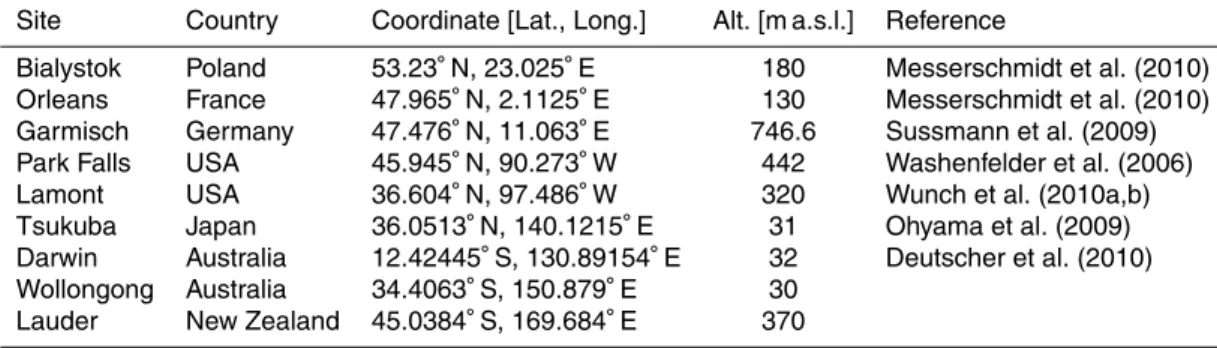
3.2 FTS sites used for validation

The g-b FTS data at 9 sites are used in this analysis. Figure 1 shows the location of the FTS sites which are used in the present study. FTS sites are located in Asia, Oceania, Europe, and North America. Table 1 summarizes the spatial coordinates of

25

(9)

AMTD

3, 5613–5643, 2010

I. Morino et al.

◭ ◮

Discussion

P

a

per

|

Dis

cussion

P

a

per

|

Discussion

P

a

per

|

Discussio

n

P

a

per

|

4 Results of initial validation

4.1 GOSAT product selection for validation

The GOSAT SWIRXCO2andXCH4products used here are Ver.01.xx. The retrieval

algo-rithm for Ver.01.xx uses band 1 (12 900–13 200 cm−1) and band 2 (5800–6400 cm−1) to simultaneously estimate X_CO2 and X_CH4. In addition, the water vapor profile and

5

aerosol optical depth (AOD) at a wavelength of 1.6 µm are retrieved. Band 3 is used for selecting scenes with cirrus clouds which CAI can not detect (Yoshida et al., 2010). TheXCO2andXCH4 data shown here (general public users, or GU subset) are filtered

for AOD less than 0.5. As a plane-parallel atmosphere is assumed in the retrieval, data with solar zenith angles greater than 70◦ are not processed, and data over high

10

mountain ranges such as the Rockies, the Andes, and the Himalayan mountains are removed.

4.2 Global distribution ofXCO2andXCH4

Figures 2 and 3 show the global distribution of GOSAT SWIRXCO2andXCH4measured

in April and October 2009. When several GOSAT data were retrieved at the same

15

observation point in the month, the latest retrieved value was overwritten in Figs. 2 and 3. There are retrievals that satisfy the filter criteria over North Africa, the Arabian Peninsula, and Australia. Data over land are obtained mainly for 10–60◦N and 15– 45◦_{S in April, and 10–50}◦_{N and 0–50}◦_{S in October. Data over ocean are retrieved} in the regions of 10◦S–30◦N in April and 40◦S–10◦N in October by observing the

20

specular reflection of sunlight in the direction of sunglint.

XCO2in April is generally higher in the Northern Hemisphere than the Southern

Hemi-sphere (Fig. 2). This is because plant photosynthesis in the Northern HemiHemi-sphere is not yet competitive with respiration in April. In October, similar XCO2 is observed in

both hemispheres. The standard deviations of monthly meanXCO2is about 1% for a

25

(10)

AMTD

3, 5613–5643, 2010

I. Morino et al.

◭ ◮

Discussion

P

a

per

|

Dis

cussion

P

a

per

|

Discussion

P

a

per

|

Discussio

n

P

a

per

XCH4in the Northern Hemisphere is higher than in the Southern Hemisphere in both

April and October 2009 (Fig. 3). ElevatedXCH4is observed from India to Japan in

Octo-ber 2009. These features are similar to those obtained by SCIAMACHY (FrankenOcto-berg et al., 2006) and simulated by an inversion model (Bergamaschi et al., 2007).

4.3 Comparisons between g-b FTS data and GOSAT TANSO-FTS SWIR data

5

GOSAT TANSO-FTS SWIR data are compared with the g-b FTS data at 9 TCCON sites (Fig. 1). We illustrate here the time series of the TANSO-FTS SWIR Level 2 data and g-b FTS data and their scatter diagrams forXCO2andXCH4. The g-b FTS data are the

mean values and standard deviations (one sigma) measured at each FTS site within 30 min of GOSAT overpass time (at most sites, around 13:00 LT). The GOSAT data are

10

selected within about one to three degrees rectangular area centered at each FTS site depending on the geophysical distribution of land and sea. As much as possible, we used only the GOSAT data retrieved over flat land.

4.3.1 XCO2

The time series of the GOSAT and g-b FTS data forXCO2 are shown on the left and

15

their scatter diagram on the right in Figs. 4 and 5g,h. In the scatter diagram, we plotted data when g-b FTS data were collected within 30 min of the GOSAT overpass time and corresponding GOSAT XCO2 values were successfully retrieved. Only a few GOSAT

data are available for comparison with Bialystok, Garmisch, Park Falls and Lauder. Darwin FTS data were not obtained since 2010 due to mechanical problems with the

20

sun tracker. X_CO2 retrieved from GOSAT SWIR measured near Orleans, Lamont and Tsukuba sites are higher in boreal spring and lower in autumn (Figs. 4b, 5e and f). Although GOSAT data are generally biased low compared with the g-b FTS, similar seasonal variations are observed. A clear seasonality over the Northern Hemisphere can also be seen in the horizontal maps of Fig. 2. In contrast, the seasonal variation

(11)

AMTD

3, 5613–5643, 2010

I. Morino et al.

◭ ◮

Discussion

P

a

per

|

Dis

cussion

P

a

per

|

Discussion

P

a

per

|

Discussio

n

P

a

per

|

of g-b FTSXCO2in the Southern Hemisphere (i.e., Darwin, Wollongong, and Lauder)

is weak (Fig. 5g,h and i) as expected due to smaller contribution of the continents. Figure 6 shows the scatter diagram between the GOSAT data and the g-b FTS data for all sites, and Table 2 summarizes the difference of the GOSAT data to the g-b FTS data at each site. The difference of the GOSAT data to the g-b FTS data is

5

−8.85±4.75 ppm or−2.3±1.2%.

4.3.2 XCH4

The time series of the GOSAT and g-b FTS data for XCH4 are shown on the left and

their scatter diagrams on the right in Figs. 7 and 8. The GOSAT retrievals are quite similar to the g-b FTS data for each site. Furthermore, the bias of XCH4 is smaller

10

than that of XCO2. In Lamont and Orleans, XCH4 levels obtained from GOSAT SWIR

are higher in boreal autumn. The g-b FTS data ofXCH4 over Tsukuba have a peak in

summer rather than autumn.

Figure 9 shows the scatter diagram between the GOSAT data and the g-b FTS data for all sites. The difference between the GOSAT data and the g-b FTS data at each

15

site is shown in Table 3. The difference of the GOSAT data to the g-b FTS data is

−20.4±18.9 ppb or−1.2±1.1%.

4.4 Latitudinal distributions of zonal averaged GOSAT SWIRXCO2andXCH4

In Sect. 4.3, g-b FTS data recorded within 30 min of the GOSAT overpass were used for the validation. To obtain larger number of samples and depict the latitudinal features,

20

we calculated monthly mean X_CO2 and X_CH4 of g-b FTS data obtained within 30 min of the time when GOSAT is supposed to overpass for all days, including the days when GOSAT does not overpass each site. In addition, monthly mean values of zonal averaged GOSAT data, based on all data obtained, are calculated in each 15 degree latitudinal band.

(12)

AMTD

3, 5613–5643, 2010

I. Morino et al.

◭ ◮

Discussion

P

a

per

|

Dis

cussion

P

a

per

|

Discussion

P

a

per

|

Discussio

n

P

a

per

Latitudinal distributions of monthly means of zonal averaged GOSAT SWIR and g-b FTS data of XCO2 in April and October 2009 are shown in Fig. 10. Both data sets

show that XCO2 is higher in the Northern Hemisphere compared with the Southern

Hemisphere in April and the difference between the hemispheres is small in October. The difference ofXCO2 between April and October is about 5 ppm in the northern mid

5

latitudes for both data sets. The zonal means of GOSAT data are reasonably consistent with those of the reference values.

Figure 11 shows latitudinal distributions of monthly means of zonal averaged GOSAT SWIR and g-b FTS data ofXCH4for April and October 2009. XCH4is

character-ized by relatively high concentration in the Northern Hemisphere in April and October.

10

Moreover, the bias is smaller than that ofXCO2. In particular, concentration ofXCH4 of

GOSAT data is a good agreement with that of g-b FTS sites in April. BothXCH4data in

October are similar distribution, though a striking difference is seen near 50–60◦N.

5 Discussion

In this study, we performed the validation of GOSAT TANSO-FTS SWIRXCO2andXCH4.

15

In Ver.01.xx, the influence of aerosols has been markedly reduced compared with ear-lier versions of the retrievals (Yokota et al., 2009). However, bias due to aerosols and thin cirrus clouds still exists because the anomalously lowXCO2retrievals as illustrated

in Fig. 2. In the future, we plan to investigate interferences by aerosols and thin cirrus clouds using aerosol lidars and/or sky-radiometers at selected FTS sites.

20

The negative bias of about 9 ppm or 2.3% in the GOSAT TANSO-FTS SWIR data of XCO2 is not still understood. It may result from unknown spectroscopic parameters of

O₂ and CO₂ or error in the TANSO-FTS calibration. In the case of the GOSAT SWIR data ofXCH4, the negative bias decreased in the Ver.01.xx compared with the earlier

Ver.00.yy when the spectroscopic parameters were changed from Lyulin et al. (2009)

25

(13)

AMTD

3, 5613–5643, 2010

I. Morino et al.

◭ ◮

Discussion

P

a

per

|

Dis

cussion

P

a

per

|

Discussion

P

a

per

|

Discussio

n

P

a

per

|

The precision of the GOSAT SWIR XCO2 and XCH4 is considered to be about 1%.

The retrieval errors of XCO2 and XCH4 are on average 2 ppm and 8 ppb or about

0.5% respectively. The retrieval errors include TANSO-FTS SWIR measurement noise, smoothing error and interference error, and the main error is the measurement noise (Yoshida et al., 2010). This means that the other errors of about 0.5% are due to

5

influences of factors such as aerosols and thin cirrus clouds.

6 Conclusions

The GOSAT TANSO-FTS SWIR data of XCO2 and XCH4 in the Version 01.xx were

compared against reference data obtained with the TCCON g-b FTS sites. The GOSAT TANSO-FTS SWIR XCO2 and XCH4 were biased low by 8.85±4.75 ppm

10

(2.3±1.2%) and 20.4±18.9 ppb (1.2±1.1%) respectively than the reference values.

The precision of the GOSAT SWIRXCO2andXCH4retrievals is considered to be about

1%.

AlthoughXCO2is underestimated by approximately 9 ppm, the GOSAT retrievals and

g-b FTS data show similar seasonal behaviors over the Northern Hemisphere, higher in

15

spring and lower in autumn. The latitudinal distribution of zonal averaged GOSAT SWIR XCO2andXCH4 is broadly consistent with that of the g-b FTS. We plan further study to

address the negative bias of the GOSAT SWIR XCO2 and XCH4 as well as to better

understand the influence of aerosols and thin cirrus clouds.

Acknowledgements. We express our sincere thanks to the members of the NIES GOSAT

20

project office, data algorithm team, atmospheric transport modeling team for their useful com-ments. We thank Nobuyuki Kikuchi in NIES and Komei Yamaguchi in the Japan Weather Asso-ciation for plotting the data. This work was funded by the Ministry of the Environment in Japan. We also thank NASA’s Terrestrial Ecology Program and the Orbiting Carbon Observatory for their support of TCCON, and acknowledge support from the EU within the projects GEOMON

25

(14)

AMTD

3, 5613–5643, 2010

I. Morino et al.

◭ ◮

Discussion

P

a

per

|

Dis

cussion

P

a

per

|

Discussion

P

a

per

|

Discussio

n

P

a

per

References

Baker, D. F., Law, R. M., Gurney, K. R., Rayner, P., Peylin, P., Denning, A. S., Bousquet, P., Bruhwiler, L., Chen, Y.-H., Ciais, P., Fung, I. Y., Heimann, M., John, J., Maki, T., Maksyu-tov, S., Masarie, K., Prather, M., Pak, B., Taguchi, S., and Zhu, Z.: TransCom 3 inversion intercomparison: Impact of transport model errors on the interannual variability of regional

5

CO₂fluxes, 1988–2003, Global Biogeochem. Cy., 20, GB1002, doi:10.1029/2004GB002439, 2006.

Bergamaschi, P., Frankenberg, C., Meirink, J. F., Krol, M., Dentener, F., Wagner, T., Platt, U., Kaplan, J. O., K ¨orner, S., Heimann, M., Dlugokencky, E. J., and Goede, A.: Satellite chartog-raphy of atmospheric methane from SCIAMACHY on board ENVISAT: 2. Evaluation based

10

on inverse model simulations, J. Geophys. Res., 112, D02304, doi:10.1029/2006JD007268, 2007.

Chahine, M., Barnet, C., Olsen, E. T., Chen, L., and Maddy, E.: On the determination of atmo-spheric minor gases by the method of vanishing partial derivatives with application to CO₂, Geophy. Res. Lett., 32, L22803, doi:10.1029/2005GL024165, 2005.

15

Cox, P. M., Betts, R. A., Jones, C. D., Spall, S. A., and Totterdell, I. J.: Acceleration of global warming due to carbon-cycle feedbacks in a coupled climate model, Nature, 408, 184–187, 2000.

Deutscher, N. M., Griffith, D. W. T., Bryant, G. W., Wennberg, P. O., Toon, G. C., Washenfelder, R. A., Keppel-Aleks, G., Wunch, D., Yavin, Y., Allen, N. T., Blavier, J.-F., Jim ´enez, R., Daube,

20

B. C., Bright, A. V., Matross, D. M., Wofsy, S. C., and Park, S.: Total column CO₂ measure-ments at Darwin, Australia - site description and calibration against in situ aircraft profiles, Atmos. Meas. Tech., 3, 947–958, doi:10.5194/amt-3-947-2010, 2010.

Dils, B., De Mazi `ere, M., M ¨uller, J. F., Blumenstock, T., Buchwitz, M., de Beek, R., Demoulin, P., Duchatelet, P., Fast, H., Frankenberg, C., Gloudemans, A., Griffith, D., Jones, N.,

Kerzen-25

macher, T., Kramer, I., Mahieu, E., Mellqvist, J., Mittermeier, R. L., Notholt, J., Rinsland, C. P., Schrijver, H., Smale, D., Strandberg, A., Straume, A. G., Stremme, W., Strong, K., Suss-mann, R., Taylor, J., van den Broek, M., Velazco, V., Wagner, T., Warneke, T., Wiacek, A., and Wood, S.: Comparisons between SCIAMACHY and ground-based FTIR data for total columns of CO, CH₄, CO₂and N₂O, Atmos. Chem. Phys., 6, 1953–1976,

doi:10.5194/acp-30

(15)

AMTD

3, 5613–5643, 2010

I. Morino et al.

◭ ◮

Discussion

P

a

per

|

Dis

cussion

P

a

per

|

Discussion

P

a

per

|

Discussio

n

P

a

per

|

Frankenberg, C., Meirink, J. F., Bergamaschi, P., Goede, A. P. H., Heimann, M., K ¨orner, S., Platt, U., van Weele, M., and Wagner, T.: Satellite chartography of atmospheric methane from SCIAMACHY on board ENVISAT: Analysis of the years 2003 and 2004, J. Geophys. Res., 111, D07303, doi:10.1029/2005JD006235, 2006.

Houweling, S., Breon, F.-M., Aben, I., R ¨odenbeck, C., Gloor, M., Heimann, M., and Ciais, P.:

5

Inverse modeling of CO₂sources and sinks using satellite data: a synthetic inter-comparison of measurement techniques and their performance as a function of space and time, Atmos. Chem. Phys., 4, 523–538, doi:10.5194/acp-4-523-2004, 2004.

Intergovernmental Panel on Climate Change (IPCC): Climate change 2007: The Physical Sci-ence Basis: Contribution of Working Group I to the Fourth Assessment Report of the

In-10

tergovernmental Panel on Climate Change, edited by: Solomon, S., Qin, S., Manning, M., Chen, Z., Marquis, M., Averyt, K. B., Tignor, M., and Miller, H. L., Cambridge University Press, Cambridge, UK and New York, NY, USA, 996 pp., 2007.

Ishida, H. and Nakajima, T. Y.: Development of an unbiased cloud detection al-gorithm for a spaceborne multispectral imager, J. Geophys. Res., 114, D07206,

15

doi:10.1029/2008JD010710, 2009.

Kulawik, S. S., Jones, D. B. A., Nassar, R., Irion, F. W., Worden, J. R., Bowman, K. W., Machida, T., Matsueda, H., Sawa, Y., Biraud, S. C., Fischer, M. L., and Jacobson, A. R.: Characteri-zation of Tropospheric Emission Spectrometer (TES) CO₂for carbon cycle science, Atmos. Chem. Phys., 10, 5601–5623, doi:10.5194/acp-10-5601-2010, 2010.

20

Kuze, A., Suto, H., Nakajima, M., and Hamazaki, T.: Thermal and near infrared sensor for carbon observation Fourier-transform spectrometer on the Greenhouse Gases Observing Satellite for greenhouse gases monitoring, Appl. Optics, 48, 6716–6733, 2009.

Lyulin, O. M., Nikitin, A. V., Perevalov, V. I., Morino, I., Yokota, T., Kumazawa, R., and Watanabe, T.: Measurements of N₂- and O₂-broadening and shifting parameters of methane spectral

25

lines in the 5550–6236 cm−1

region, J. Quant. Spectrosc. Ra., 110, 654–668, 2009.

Messerschmidt, J., Macatangay, R., Notholt, J., Petri, C., Warneke, T., and Weinzierl, C.: Side by side measurements of CO₂by ground-based Fourier transform spectrometry (FTS), Tel-lus B, 62, 749–758, 2010.

Miller, C. E., Crisp, D., DeCola, P. L., Olsen, S. C., Randerson, J. T., Michalak, A. M., Alkhaled,

30

(16)

AMTD

3, 5613–5643, 2010

I. Morino et al.

◭ ◮

Discussion

P

a

per

|

Dis

cussion

P

a

per

|

Discussion

P

a

per

|

Discussio

n

P

a

per

and Law, R. M.: Precision requirements for space-basedXCO2data, J. Geophys. Res., 112, D10314, doi:10.1029/2006JD007659, 2007.

Ohyama, H., Morino, I., Nagahama, T., Machida, T., Suto, H., Oguma, H., Sawa, Y., Matsueda, H., Sugimoto, N., Nakane, H., and Nakagawa, K.: Column-averaged volume mixing ratio of CO₂measured with ground-based Fourier transform spectrometer at Tsukuba, J. Geophys.

5

Res., 114, D18303, doi:10.1029/2008JD011465, 2009.

Rayner, P. J. and O’Brien, D. M.: The utility of remotely sensed CO₂ concentration data in surface source inversions, Geophys. Res. Lett., 28, 175–178, 2001.

Rothman, L. S., Gordon, I. E., Barbe, A., Benner, D. C., Bernath, P. F., Birk, M., Boudon, V., Brown, L. R., Campargue, A., Champion, J.-P., Chance, K., Coudert, L. H., Dana, V., Devi,

10

V. M., Fally, S., Flaud, J.-M., Gamache, R. R., Goldman, A., Jacquemart, D., Kleiner, I., Lacome, N., Lafferty, W. J., Mandin, J.-Y., Massie, S. T., Mikhailenko, S. N., Miller, C. E., Moazzen-Ahmadi, N., Naumenko, O. V., Nikitin, A. V., Orphal, J., Perevalov, V. I., Perrin, A., Predoi-Cross, A., Rinsland, C. P., Rotger, M., ˇSimeˇckov ´a, M., Smith, M. A. H., Sung, K., Tashkun, S. A., Tennyson, J., Toth, R. A., Vandaele, A. C., and Auwera, J. V.: The

15

HITRAN 2008 molecular spectroscopic database, J. Quant. Spectrosc. Ra., 110, 533–572, 2009.

Saitoh, N., Imasu, R., Ota, Y., and Niwa, Y.: CO₂ retrieval algorithm for the thermal infrared spectra of the Greenhouse Gases Observing Satellite: Potential of retrieving CO₂ vertical profile from high-resolution FTS sensor, J. Geophys. Res., 114, D17305,

20

doi:10.1029/2008JD011500, 2009.

Schneising, O., Buchwitz, M., Burrows, J. P., Bovensmann, H., Reuter, M., Notholt, J., Macatan-gay, R., and Warneke, T.: Three years of greenhouse gas column-averaged dry air mole frac-tions retrieved from satellite - Part 1: Carbon dioxide, Atmos. Chem. Phys., 8, 3827–3853, doi:10.5194/acp-8-3827-2008, 2008.

25

Sussmann, R., Stremme, W., Buchwitz, M., and de Beek, R.: Validation of EN-VISAT/SCIAMACHY columnar methane by solar FTIR spectrometry at the Ground-Truthing Station Zugspitze, Atmos. Chem. Phys., 5, 2419–2429, doi:10.5194/acp-5-2419-2005, 2005.

Sussmann, R., Rettinger, M., and Borsdorff, T.: The new TCCON-FTS site at Garmisch,

Ger-30

(17)

AMTD

3, 5613–5643, 2010

I. Morino et al.

◭ ◮

Discussion

P

a

per

|

Dis

cussion

P

a

per

|

Discussion

P

a

per

|

Discussio

n

P

a

per

|

Toon, G. C., Farmer, C. B., Schaper, P. W., Lowes, L. L., and Norton, R. H.: Composition measurements of the 1989 Arctic winter stratosphere by airborne infrared solar absorption spectroscopy, J. Geophys. Res., 97, 7939–7961, doi:10.1029/91JD03114, 1992.

Washenfelder, R. A., Toon, G. C., Blavier, J.-F., Yang, Z., Allen, N. T., Wennberg, P. O., Vay, S. A., Matross, D. M., and Daube, B. C.: Carbon dioxide column abundances at the Wisconsin

5

Tall Tower site, J. Geophys. Res., 111, D22305, doi:10.1029/2006JD007154, 2006.

WMO: The state of greenhouse gases in the atmosphere using global observations through 2008, WMO Greenhouse Gas Bulletin, No. 5, 2009.

World Data Centre for Greenhouse Gases: WMO Global Watch World Data Centre for Green-house Gases, http://gaw.kishou.go.jp/wdcgg/wdcgg.html/, last access: December, 2010.

10

Wunch, D., Toon, G. C., Wennberg, P. O., Wofsy, S. C., Stephens, B. B., Fischer, M. L., Uchino, O., Abshire, J. B., Bernath, P., Biraud, S. C., Blavier, J.-F. L., Boone, C., Bowman, K. P., Browell, E. V., Campos, T., Connor, B. J., Daube, B. C., Deutscher, N. M., Diao, M., Elkins, J. W., Gerbig, C., Gottlieb, E., Gri_ffith, D. W. T., Hurst, D. F., Jim ´enez, R., Keppel-Aleks, G., Kort, E. A., Macatangay, R., Machida, T., Matsueda, H., Moore, F., Morino, I., Park, S.,

15

Robinson, J., Roehl, C. M., Sawa, Y., Sherlock, V., Sweeney, C., Tanaka, T., and Zondlo, M. A.: Calibration of the Total Carbon Column Observing Network using aircraft profile data, Atmos. Meas. Tech., 3, 1351–1362, doi:10.5194/amt-3-1351-2010, 2010a.

Wunch, D., Toon, G. C., Blavier, J.-F. L., Washenfelder, R. A., Notholt, J., Connor, B. J., Griffith, D. W. T., Sherlock, V., and Wennberg, P. O.: The Total Carbon Column Observing

Net-20

work (TCCON), Philos. T. Roy. Soc. A, in press, 2010b.

Yokota, T., Yoshida, Y., Eguchi, N., Ota, Y., Tanaka, T., Watanabe, H., and Maksyutov, S.: Global concentrations of CO₂ and CH₄ retrieved from GOSAT: First preliminary results, SOLA, 5, 160–163, 2009.

Yoshida, Y., Ota, Y., Eguchi, N., Kikuchi, N., Nobuta, K., Tran, H., Morino, I., and Yokota, T.:

25

(18)

AMTD

3, 5613–5643, 2010

I. Morino et al.

◭ ◮

Discussion

P

a

per

|

Dis

cussion

P

a

per

|

Discussion

P

a

per

|

Discussio

n

P

a

per

Table 1.g-b FTS sites used for GOSAT product validation.

Site Country Coordinate [Lat., Long.] Alt. [m a.s.l.] Reference

Bialystok Poland 53.23◦_{N, 23.025}◦_E ₁₈₀ _{Messerschmidt et al. (2010)}

Orleans France 47.965◦_{N, 2.1125}◦_E ₁₃₀ _{Messerschmidt et al. (2010)}

Garmisch Germany 47.476◦_{N, 11.063}◦_E _746.6 _{Sussmann et al. (2009)}

Park Falls USA 45.945◦_{N, 90.273}◦_W ₄₄₂ _{Washenfelder et al. (2006)}

Lamont USA 36.604◦_{N, 97.486}◦_W ₃₂₀ _{Wunch et al. (2010a,b)}

Tsukuba Japan 36.0513◦_{N, 140.1215}◦_E ₃₁ _{Ohyama et al. (2009)}

Darwin Australia 12.42445◦_{S, 130.89154}◦_E ₃₂ _{Deutscher et al. (2010)}

Wollongong Australia 34.4063◦_{S, 150.879}◦_E ₃₀

(19)

AMTD

3, 5613–5643, 2010

I. Morino et al.

◭ ◮

Discussion

P

a

per

|

Dis

cussion

P

a

per

|

Discussion

P

a

per

|

Discussio

n

P

a

per

|

Table 2. Left side: the average and one standard deviation (1 σ) of the difference between

GOSATX_CO2and g-b FTS X_CO2for the nine TCCON sites. Right side: the average and one standard deviation (1σ) of the di_fference normalized to g-b FTSX_CO2(given in percent). Note that the number of data listed here indicates the count of valid cases in which g-b FTS data were collected within 30 min of the GOSAT overpass time and corresponding GOSAT XCO2 values were successfully retrieved.

Sites (GOSAT SWIRXCO2)–(g-b FTSXCO2) (GOSAT SWIRXCO2)–(g-b FTSXCO2)

(g-b FTSX_CO2)

Number Average 1σ Average 1σ

of data (ppm) (ppm) (%) (%)

Bialystok 1 5.01 – 1.32 –

Orleans 14 −12.85 3.79 −3.33 0.99

Garmisch 3 −7.78 3.78 −2.00 0.96

Park Falls 1 −6.05 – −1.58 –

Lamont 11 −10.31 4.80 −2.65 1.23

Tsukuba 13 −6.38 2.75 −1.64 0.71

Darwin 6 −6.09 2.61 −1.58 0.68

Wollongong 11 −8.77 4.74 −2.28 1.23

Lauder 2 −7.45 0.15 −1.94 0.04

(20)

AMTD

3, 5613–5643, 2010

I. Morino et al.

◭ ◮

Discussion

P

a

per

|

Dis

cussion

P

a

per

|

Discussion

P

a

per

|

Discussio

n

P

a

per

Table 3.As in Table 2 except forX_CH4.

Sites (GOSAT SWIRXCH4)–(g-b FTSXCH4) (GOSAT SWIRXCH4)–(g-b FTSXCH4)

(g-b FTSXCH4)

Number Average 1σ Average 1σ

of data (ppm) (ppm) (%) (%)

Bialystok 1 0.0227 – 1.29 –

Orleans 14 −0.0367 0.0178 −2.06 1.00

Garmisch 3 −0.0114 0.0160 −0.64 0.90

Park Falls 1 −0.0120 – −0.66 –

Lamont 11 −0.0230 0.0181 −1.28 1.01

Tsukuba 13 −0.0120 0.0115 −0.67 0.64

Darwin 6 −0.0080 0.0089 −0.46 0.51

Wollongong 11 −0.0235 0.0190 −1.34 1.08

Lauder 2 −0.0067 0.0003 −0.39 0.01

(21)

AMTD

3, 5613–5643, 2010

I. Morino et al.

◭ ◮

Discussion

P

a

per

|

Dis

cussion

P

a

per

|

Discussion

P

a

per

|

Discussio

n

P

a

per

|

(22)

AMTD

3, 5613–5643, 2010

I. Morino et al.

◭ ◮

Discussion

P

a

per

|

Dis

cussion

P

a

per

|

Discussion

P

a

per

|

Discussio

n

P

a

per

(a)

(b)

(23)

AMTD

3, 5613–5643, 2010

I. Morino et al.

◭ ◮

Discussion

P

a

per

|

Dis

cussion

P

a

per

|

Discussion

P

a

per

|

Discussio

n

P

a

per

|

(a)

(b)

(24)

AMTD

3, 5613–5643, 2010

I. Morino et al.

Title Page Abstract Introduction Conclusions References Tables Figures ◭ ◮ ◭ ◮ Back Close Full Screen / Esc Printer-friendly Version Interactive Discussion Discussion P a per | Dis cussion P a per | Discussion P a per | Discussio n P a per (a) 350 360 370 380 390 400 410

2009/ 1/ 1 2009/ 5/ 27 2009/ 10/ 20 2010/ 3/ 15 2010/ 8/ 8 2011/ 1/ 1 Date

XCO2

( p p m ) 350 360 370 380 390 400 410

350 360 370 380 390 400 410 g-b FTS XCO2 (ppm)

G O S A T S W IR XC O 2 ( p p m ) Bialystok Bialystok (b) 350 360 370 380 390 400 410

2009/ 1/ 1 2009/ 5/ 27 2009/ 10/ 20 2010/ 3/ 15 2010/ 8/ 8 2011/ 1/ 1 Date

XCO

2 ( p p m ) 350 360 370 380 390 400 410

350 360 370 380 390 400 410 g-b FTS XCO2 (ppm)

G O S A T S W IR XC O 2 ( p p m ) Orleans Orleans (c) 350 360 370 380 390 400 410

2009/ 1/ 1 2009/ 5/ 27 2009/ 10/ 20 2010/ 3/ 15 2010/ 8/ 8 2011/ 1/ 1 Date

XCO

2 ( p p m ) 350 360 370 380 390 400 410

350 360 370 380 390 400 410 g-b FTS XCO2 (ppm)

G O S A T S W IR XC O 2 ( p p m ) Garmisch Garmisch (d) 350 360 370 380 390 400 410

2009/ 1/ 1 2009/ 5/ 27 2009/ 10/ 20 2010/ 3/ 15 2010/ 8/ 8 2011/ 1/ 1 Date

XCO

2 ( p p m ) 350 360 370 380 390 400 410

350 360 370 380 390 400 410 g-b FTS XCO2 (ppm)

G O S A T S W IR XC O 2 ( p p m )

Park Falls Park Falls

(25)

AMTD

3, 5613–5643, 2010

I. Morino et al.

Title Page Abstract Introduction Conclusions References Tables Figures ◭ ◮ ◭ ◮ Back Close Full Screen / Esc Printer-friendly Version Interactive Discussion Discussion P a per | Dis cussion P a per | Discussion P a per | Discussio n P a per | (e) 350 360 370 380 390 400 410

2009/ 1/ 1 2009/ 5/ 27 2009/ 10/ 20 2010/ 3/ 15 2010/ 8/ 8 2011/ 1/ 1 Date

XCO2

( p p m ) 350 360 370 380 390 400 410

350 360 370 380 390 400 410 g-b FTS XCO2 (ppm)

G O S A T S W IR XC O 2 ( p p m ) Lamont Lamont (f) 350 360 370 380 390 400 410

2009/ 1/ 1 2009/ 5/ 27 2009/ 10/ 20 2010/ 3/ 15 2010/ 8/ 8 2011/ 1/ 1 Date

XCO2

( p p m ) 350 360 370 380 390 400 410

350 360 370 380 390 400 410 g-b FTS XCO2 (ppm)

G O S A T S W IR X C O 2 ( p p m ) Tsukuba Tsukuba (g) 350 360 370 380 390 400 410

2009/ 1/ 1 2009/ 5/ 27 2009/ 10/ 20 2010/ 3/ 15 2010/ 8/ 8 2011/ 1/ 1 Date

XCO2

( p p m ) 350 360 370 380 390 400 410

350 360 370 380 390 400 410 g-b FTS XCO2 (ppm)

G O S A T S W IR XC O 2 ( p p m ) Darwin Darwin (h) 350 360 370 380 390 400 410

2009/ 1/ 1 2009/ 5/ 27 2009/ 10/ 20 2010/ 3/ 15 2010/ 8/ 8 2011/ 1/ 1 Date

XCO2

( p p m ) 350 360 370 380 390 400 410

350 360 370 380 390 400 410 g-b FTS XCO2 (ppm)

G O S A T S W IR XC O 2 ( p p m ) Wollongong Wollongong (i) 350 360 370 380 390 400 410

2009/ 1/ 1 2009/ 5/ 27 2009/ 10/ 20 2010/ 3/ 15 2010/ 8/ 8 2011/ 1/ 1 Date

XCO2

( p p m ) 350 360 370 380 390 400 410

350 360 370 380 390 400 410 g-b FTS XCO2 (ppm)

G O S A T S W IR XC O 2 ( p p m ) Lauder Lauder

Fig. 5. As in Fig. 4 except for (e) Lamont, (f) Tsukuba, (g) Darwin, (h) Wollongong, and

(26)

AMTD

3, 5613–5643, 2010

I. Morino et al.

◭ ◮

Discussion

P

a

per

|

Dis

cussion

P

a

per

|

Discussion

P

a

per

|

Discussio

n

P

a

per

360 370 380 390 400

g-b FTS XC O 2 (ppm)

G

O

S

A

T

S

W

IR

X

C

O

2

(

p

m

)

Bialystok

Orleans

Garmisch

ParkFalls

Lamont

Tsukuba

Darw in

Wollongong

Lauder

(27)

AMTD

3, 5613–5643, 2010

I. Morino et al.

Title Page Abstract Introduction Conclusions References Tables Figures ◭ ◮ ◭ ◮ Back Close Full Screen / Esc Printer-friendly Version Interactive Discussion Discussion P a per | Dis cussion P a per | Discussion P a per | Discussio n P a per | (a) 1.5 1.6 1.7 1.8 1.9 2.0

2009/ 1/ 1 2009/ 5/ 27 2009/ 10/ 20 2010/ 3/ 15 2010/ 8/ 8 2011/ 1/ 1 Date

XCH

4 ( p p m ) 1.5 1.6 1.7 1.8 1.9 2.0

1.5 1.6 1.7 1.8 1.9 2.0

g-b FTS XCH4 (ppm)

G O S A T S W IR X C H 4 ( p p m ) Bialystok Bialystok (b) 1.5 1.6 1.7 1.8 1.9 2.0

2009/ 1/ 1 2009/ 5/ 27 2009/ 10/ 20 2010/ 3/ 15 2010/ 8/ 8 2011/ 1/ 1 Date

XCH4

( p p m ) 1.5 1.6 1.7 1.8 1.9 2.0

1.5 1.6 1.7 1.8 1.9 2.0

g-b FTS XCH4 (ppm)

G O S A T S W IR X C H 4 ( p p m ) Orleans Orleans (c) 1.5 1.6 1.7 1.8 1.9 2.0

2009/ 1/ 1 2009/ 5/ 27 2009/ 10/ 20 2010/ 3/ 15 2010/ 8/ 8 2011/ 1/ 1 Date

XCH

4 ( p p m ) 1.5 1.6 1.7 1.8 1.9 2.0

1.5 1.6 1.7 1.8 1.9 2.0

g-b FTS XCH4 (ppm)

G O S A T S W IR X C H 4 ( p p m ) Garmisch Garmisch (d) 1.5 1.6 1.7 1.8 1.9 2.0

2009/ 1/ 1 2009/ 5/ 27 2009/ 10/ 20 2010/ 3/ 15 2010/ 8/ 8 2011/ 1/ 1 Date

XCH4

( p p m ) 1.5 1.6 1.7 1.8 1.9 2.0

1.5 1.6 1.7 1.8 1.9 2.0

g-b FTS XCH4 (ppm)

G O S A T S W IR X C H 4 ( p p m )

Park Falls Park Falls

Fig. 7. Time series of GOSAT TANSO-FTS SWIR (blue triangles) and g-b FTS (pink squares)

(28)

AMTD

3, 5613–5643, 2010

I. Morino et al.

Title Page Abstract Introduction Conclusions References Tables Figures ◭ ◮ ◭ ◮ Back Close Full Screen / Esc Printer-friendly Version Interactive Discussion Discussion P a per | Dis cussion P a per | Discussion P a per | Discussio n P a per (e) 1.5 1.6 1.7 1.8 1.9 2.0

2009/ 1/ 1 2009/ 5/ 27 2009/ 10/ 20 2010/ 3/ 15 2010/ 8/ 8 2011/ 1/ 1 Date

XCH

4 ( p p m ) 1.5 1.6 1.7 1.8 1.9 2.0

1.5 1.6 1.7 1.8 1.9 2.0 g-b FTS XCH4 (ppm)

G O S A T S W IR XC H 4 ( p p m ) Lamont Lamont (f) 1.5 1.6 1.7 1.8 1.9 2.0

2009/ 1/ 1 2009/ 5/ 27 2009/ 10/ 20 2010/ 3/ 15 2010/ 8/ 8 2011/ 1/ 1 Date

XCH4

( p p m ) 1.5 1.6 1.7 1.8 1.9 2.0

1.5 1.6 1.7 1.8 1.9 2.0 g-b FTS XCH4 (ppm)

G O S A T S W IR XC H 4 ( p p m ) Tsukuba Tsukuba (g) 1.5 1.6 1.7 1.8 1.9 2.0

2009/ 1/ 1 2009/ 5/ 27 2009/ 10/ 20 2010/ 3/ 15 2010/ 8/ 8 2011/ 1/ 1 Date

XCH4

( p p m ) 1.5 1.6 1.7 1.8 1.9 2.0

1.5 1.6 1.7 1.8 1.9 2.0 g-b FTS XCH4 (ppm)

G O S A T S W IR X C H 4 ( p p m ) Darwin Darwin (h) 1.5 1.6 1.7 1.8 1.9 2.0

2009/ 1/ 1 2009/ 5/ 27 2009/ 10/ 20 2010/ 3/ 15 2010/ 8/ 8 2011/ 1/ 1 Date

XCH4

( p p m ) 1.5 1.6 1.7 1.8 1.9 2.0

1.5 1.6 1.7 1.8 1.9 2.0 g-b FTS XCH4 (ppm)

G O S A T S W IR XC H 4 ( p p m ) Wollongong Wollongong (i) 1.5 1.6 1.7 1.8 1.9 2.0

2009/ 1/ 1 2009/ 5/ 27 2009/ 10/ 20 2010/ 3/ 15 2010/ 8/ 8 2011/ 1/ 1 Date

XCH4

( p p m ) 1.5 1.6 1.7 1.8 1.9 2.0

1.5 1.6 1.7 1.8 1.9 2.0 g-b FTS XCH4 (ppm)

G O S A T S W IR X C H 4 ( p p m ) Lauder Lauder

(29)

AMTD

3, 5613–5643, 2010

I. Morino et al.

◭ ◮

Discussion

P

a

per

|

Dis

cussion

P

a

per

|

Discussion

P

a

per

|

Discussio

n

P

a

per

|

1.6 1.7 1.8 1.9

g-b FTS XC H 4 (ppm)

G

O

S

A

T

S

W

IR

X

C

H

4

(

p

m

)

Bialystok

Orleans

Garmisch

ParkFalls

Lamont

Tsukuba

Darw in

Wollongong

Lauder

(30)

AMTD

3, 5613–5643, 2010

I. Morino et al.

◭ ◮

Discussion

P

a

per

|

Dis

cussion

P

a

per

|

Discussion

P

a

per

|

Discussio

n

P

a

per

Fig. 10. Latitudinal distributions of monthly means of zonal averaged GOSAT X_CO2for each

(31)

AMTD

3, 5613–5643, 2010

I. Morino et al.

◭ ◮

Discussion

P

a

per

|

Dis

cussion

P

a

per

|

Discussion

P

a

per

|

Discussio

n

P

a

per

|