www.the-cryosphere.net/9/1895/2015/ doi:10.5194/tc-9-1895-2015
© Author(s) 2015. CC Attribution 3.0 License.
CryoSat-2 delivers monthly and inter-annual
surface elevation change for Arctic ice caps
L. Gray1, D. Burgess2, L. Copland1, M. N. Demuth2, T. Dunse3, K. Langley3, and T. V. Schuler3
1Department of Geography, University of Ottawa, Ottawa, K1N 6N5, Canada 2Natural Resources Canada, Ottawa, Canada
3Department of Geosciences, University of Oslo, Oslo, Norway
Correspondence to:L. Gray ([email protected])
Received: 29 April 2015 – Published in The Cryosphere Discuss.: 26 May 2015
Revised: 15 August 2015 – Accepted: 3 September 2015 – Published: 25 September 2015
Abstract. We show that the CryoSat-2 radar altimeter can provide useful estimates of surface elevation change on a variety of Arctic ice caps, on both monthly and yearly timescales. Changing conditions, however, can lead to a varying bias between the elevation estimated from the radar altimeter and the physical surface due to changes in the ratio of subsurface to surface backscatter. Under melting condi-tions the radar returns are predominantly from the surface so that if surface melt is extensive across the ice cap estimates of summer elevation loss can be made with the frequent coverage provided by CryoSat-2. For example, the average summer elevation decreases on the Barnes Ice Cap, Baf-fin Island, Canada were 2.05±0.36 m (2011), 2.55±0.32 m (2012), 1.38±0.40 m (2013) and 1.44±0.37 m (2014), losses which were not balanced by the winter snow accu-mulation. As winter-to-winter conditions were similar, the net elevation losses were 1.0±0.20 m (winter 2010/11 to winter 2011/12), 1.39±0.20 m (2011/12 to 2012/13) and 0.36±0.20 m (2012/13 to 2013/14); for a total surface el-evation loss of 2.75±0.20 m over this 3-year period. In con-trast, the uncertainty in height change from Devon Ice Cap, Canada, and Austfonna, Svalbard, can be up to twice as large because of the presence of firn and the possibility of a varying bias between the true surface and the detected elevation due to changing year-to-year conditions. Nevertheless, the sur-face elevation change estimates from CryoSat for both ice caps are consistent with field and meteorological measure-ments.
1 Introduction
To test and validate the CS2 altimeter, ESA developed the airborne ASIRAS Ku-band (13.5 GHz) radar altimeter. ASIRAS has been operated during field campaigns under the CryoSat Validation Experiment (CryoVex) at selected sites before and after the launch of the satellite. One of the most interesting revelations of the ASIRAS data has been the demonstration of variability in relative surface and subsur-face returns in a variety of locations including Devon Ice Cap in Canada, Greenland and Austfonna in Svalbard (Hawley et al., 2006, 2013; Helm et al., 2007; Brandt et al., 2008; De la Pena et al., 2010). The time variation of the ASIRAS return signals from the surface and near surface (the “waveforms”) can and does vary significantly from year-to-year at the same geographic position, and in any one year with changing po-sition across the ice cap. During cold conditions in spring, the maximum return need not be from the snow surface, but could be from the previous summer surface, or strong density contrasts within the snow pack such as those manifested by buried weathering crusts or refrozen percolating meltwater (e.g. Bell et al., 2008). Changes in snowpack characteristics, dependent on past meteorological conditions, could therefore affect the relative strength of the surface and volume compo-nent of the CS2 return signal and affect the bias between the elevation measured by CS2 and the true surface.
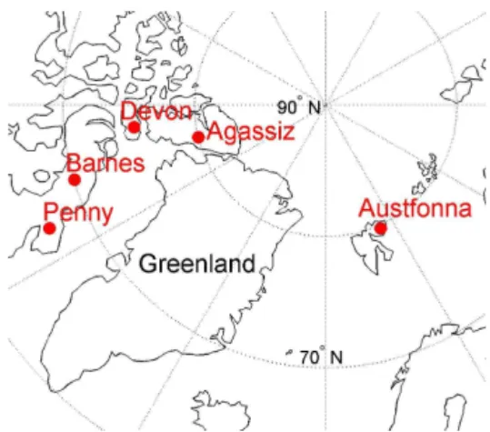
In this study we use all available SARIn data from July 2010 to December 2014 to undertake the first systematic measurement by spaceborne radar of elevation change on a variety of ice caps across the Canadian and Norwegian Arctic (Fig. 1) representing a wide range of climate regimes. Em-phasis is placed on CS2 results from Devon and Austfonna as both ice caps were selected by ESA as designated cali-bration and/or validation sites, and a wide range of ground and airborne validation data sets are available. SARIn data are also used to measure height changes on Penny, Agassiz and Barnes ice caps to illustrate the wide applicability of the method in areas where there is less data available for surface validation. Together with the recent CS2 work on Greenland and Antarctica (McMillan et al., 2014a; Helm et al., 2014), this illustrates the power of the new interferometric mode of the CS2 altimeter to provide useful information in an all-weather, day–night situation.
Our emphasis in this paper is to demonstrate that CS2 can measure elevation and elevation change on relatively small ice caps, even with differing surface conditions, and for some on a monthly timescale. The many complications associated with converting the CS2 elevation change data to an ice cap wide mass balance will be treated in future papers.
2 Study areas
We begin by describing the two ice caps, Devon and Aust-fonna, which were part of the CryoVex campaigns and which have a wide range of surface reference data. Then we discuss conditions on Barnes, Agassiz and Penny ice caps. Although
Figure 1.Location of the five ice caps measured in this study.
these ice caps have less surface reference data, they are quite different and represent a good test of the capability of the CS2 system.
2.1 The Devon Ice Cap
Occupying∼12 000 km2of eastern Devon Island, Nunavut, the main portion of the Devon Ice Cap (75◦N, 82◦W) ranges
2.2 Austfonna
Occupying ∼8100 km2 of Nordaustlandet, Svalbard,
Aust-fonna (79◦N, 23◦E) is among the largest ice caps in the
Eurasian Arctic. It consists of a main dome that reaches a maximum surface elevation of∼800 m (Moholdt and Kääb, 2012). The south-eastern basins form a continuous calving front towards the Barents Sea, while the north-western basins terminate on land or in narrow fjords (Dowdeswell, 1986). Several drainage basins are known to have surged in the past (Dowdeswell et al., 1986), including Basin-3 which en-tered renewed surge activity in autumn 2012 (McMillan et al., 2014b; Dunse et al., 2015).
Mass balance stakes indicate an equilibrium line alti-tude (ELA) of ∼450 m in the NE and ∼250 m in the SE of Austfonna (Moholdt et al., 2010). This reflects a typi-cal asymmetry in snow accumulation with the southeastern slopes receiving about twice as much precipitation as the northwestern slopes, as the Barents Sea to the east represents the primary moisture source (Pinglot et al., 2001; Taurisano et al., 2007; Dunse et al., 2009).
Despite a surface mass balance close to zero (2002–2008), the net mass balance of Austfonna has been negative at
−1.3±0.5 Gt a−1(Moholdt et al., 2010), due to calving and
retreat of the marine ice margin (Dowdeswell et al., 2008). Sporadic glacier surges, as currently seen in Basin-3 (McMil-lan et al., 2014b; Dunse et al., 2015) can significantly alter the calving flux from the ice cap. Prior to the surge of Basin-3, interior thickening at rates of ∼0.5 m a−1 and marginal
thinning of 1–3 m a−1 had been detected from repeat air-borne (1996–2002; Bamber et al., 2004) and satellite laser altimetry (2003–2008; Moholdt et al., 2010). The accumula-tion area comprises an extensive superimposed ice and wet snow zone, and in some years a percolation zone may ex-ist. The distribution of glacier facies varies significantly from year to year, a consequence of large inter-annual variability in total amount of snow and summer ablation (Dunse et al., 2009). Despite mean annual temperatures of −8.3◦C, large
temperature variations occur throughout the year and it is not uncommon for temperatures above 0◦C and rain events to
occur in winter (Schuler et al., 2014).
2.3 Barnes Ice Cap
Barnes Ice Cap (70◦N, 73◦W) is a near-stagnant ice mass
that occupies ∼5900 km2 of the central plateau of Baffin Island. It terminates at a height of ∼400–500 m around most of its perimeter, and its surface rises gradually towards the interior, reaching a maximum elevation of ∼1100 m along the summit ridge (Andrews and Barnett, 1979). In-situ surface mass balance measurements (1970–1984), in-dicate winter accumulation rates of∼0.5 m a−1snow water
equivalent (s.w.e.), and net balance for the entire ice cap of
−0.12 m a−1(Sneed et al., 2008). Mean mass loss rates have
become increasingly negative (−1.0±0.14 m a−1) up to the
present (Abdalati et al., 2004; Sneed et al., 2008; Gardner et al., 2012). In the past accumulation occurred primarily as superimposed ice (Baird, 1952), but more recently summer melt has been extensive and the ice cap has lost its entire accumulation area (Dupont et al., 2012). Similar to glaciers in the Queen Elizabeth Islands (Koerner, 2005), the surface mass balance of the Barnes Ice Cap is driven almost entirely by the magnitude and duration of summer melt (Sneed et al., 2008).
2.4 Agassiz Ice Cap
Agassiz Ice Cap (80◦N, 75◦W) occupies∼21 000 km2 of
the Arctic Cordillera on north-eastern Ellesmere Island. It ranges in elevation from sea-level, where several of the ma-jor tidewater glaciers that drain the ice cap interior termi-nate, to∼1980 m at the central summit. Ice core records ac-quired from the summit region indicate that melt rates since the early 1990’s are comparable to those last experienced in the early Holocene∼9000 years ago (Fisher et al., 2011). In situ measurements of surface mass balance indicate a long term ELA of∼1100 m with an average accumulation rate of 0.13 m w.e. a−1 over the period 1977–present. Between the
summit and the sea level outlet glaciers there is a progres-sion of ice facies similar to that described for the Devon Ice Cap.
Repeat airborne laser altimetry surveys conducted in 1995 and 2000 indicate zero change to slight thickening at high elevations, but the ice loss at lower elevations led to an esti-mate of ice cap wide thinning of∼0.07 m a−1(Abdalati et
al., 2004). More recently (2004–2009), model results con-firmed by independent satellite observations (Gardner et al., 2011) suggest the ice cap has been thinning by 0.23 m a−1.
2.5 Penny Ice Cap
Penny Ice Cap (67◦N, 66◦W) occupying∼6400 km2of the
highland region of southern Baffin Island, ranges in elevation from 0 to 1980 m and contains one main tidewater glacier, the Coronation Glacier, which calves into Baffin Bay (Zdanow-icz et al., 2012). A historical climate record derived from deep and shallow ice cores (Fisher et al., 1998, 2011) in-dicates that current melting on Penny is unprecedented in magnitude and duration for the past∼3000 years. Thickness changes derived from repeat airborne laser altimetry surveys in 1995 and 2000 indicate an average ice cap wide thinning rate of 0.15 m a−1, with a maximum thinning of∼0.5 m a−1
in the lower ablation zones (Abdalati et al., 2004). More re-cent measurements (2007–2011) indicate thinning of ∼3– 4 m a−1near the ice cap margin (330 m), amongst the
by 10◦C as a result of latent heat release due to increased
amounts of summer melt water refreezing at depth (Zdanow-icz et al., 2012).
3 Methods
3.1 CS2 SARIn data processing
All available SARIn L1b data files (processed with ESA “baseline B” software; Bouzinac, 2014) from July 2010 to the end of December 2014 were obtained from ESA for each ice cap. Although developed independently, our processing methodology to derive geocoded heights from the L1b data is similar to that described by Helm et al. (2014), so the summary below focuses on the differences between the two methods.
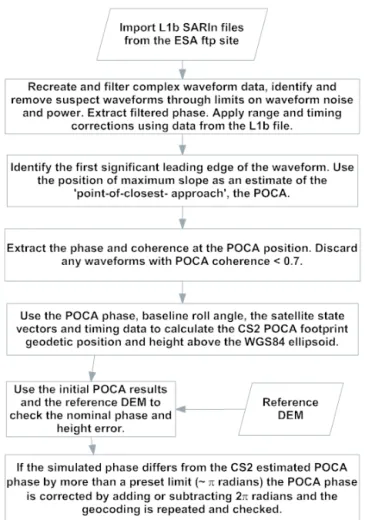
Delay Doppler processing (Raney, 1998) has been com-pleted in the down-loaded data and the resulting waveform data are included in the ESA L1b files. However, geophys-ical results, e.g. terrain footprint height and position, have not been calculated. Our processing for this stage has been developed primarily for the ice cap data acquired above, and the steps are illustrated in Fig. 2. The waveform data for each along-track position (time histories of the power, phase and coherence) include the unique “point-of-closest-approach” (POCA) followed in delay time by the sum of sur-face and subsursur-face returns from both sides of the POCA (Gray et al., 2013).
An initial examination of the L1b data showed that the received power waveforms varied in both shape and mag-nitude, and that the peak return did not necessarily follow immediately after the first strong leading edge of the return signal. This complexity is not entirely unexpected and arises due to the nature of the surface being measured, in particular the possible variation of the illuminated area at the sampling times in the receive window, and the possibility of reflections from sub-surface layers. The problem is then to identify an optimum algorithm (the “retracker”) to pick the position of the POCA from the waveform. Our approach estimates the POCA position by identifying the maximum slope on the first significant leading edge of the waveform. This is similar to the approach of Helm et al. (2014), who used a particu-lar threshold level on the first significant leading edge of the power waveform.
The choice of the threshold level retracker used by Helm et al. (2014) for their work in Greenland and Antarctica fol-lowed that of Davis (1997), who advocated a threshold re-tracker to help minimize the influence of subsurface returns on the detected elevation. Limited tests on some of the ice caps in our study have shown that a threshold retracker also produces satisfactory results but still does not totally elimi-nate the problem of a variable bias between the detected ele-vation and the physical surface. In contrast to the interior of Antarctica where near surface melt is very rare, in this study
Figure 2.Flow chart showing the methodology developed to derive terrain elevation from the L1b SARIn files.
we are dealing with surface and near-surface conditions in which there are significant spatial and temporal variations in surface roughness, near surface permittivity, and microwave penetration. Consequently, it is hard to envisage that any re-tracker would respond to the physical surface independently of the conditions of the near surface. This issue is discussed further below in the light of the airborne and CS2 results for particular ice caps, but it is doubtful that an optimum re-tracker exists for all conditions.
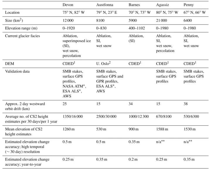
Table 1.Ice Cap information.
Devon Austfonna Barnes Agassiz Penny
Location 75◦N, 82◦W 79◦N, 23◦E 70◦N, 73◦W 80◦N, 75◦W 67◦N, 66◦W
Size (km2) 12 000 8100 5900 21 000 6400
Elevation range (m) 0–1920 0–830 400–1102 0–1980 0–1980
Current glacier facies Ablation, Ablation, Ablation, Ablation, Ablation,
superimposed ice SI, (SI) SI, SI,
(SI), wet snow wet snow, wet snow
wet snow, percolation
percolation
DEM CDED1 U. Oslo2 CDED1 CDED1 CDED1
Validation data SMB stakes, SMB stakes, SMB stakes, SMB stakes,
surface GPS surface GPS and surface GPS surface GPS
profiles, GPR profiles, profiles profiles
NASA ATM∗, ESA ALS∗, ESA ALS∗, AWS AWS
Approx. 2 day westward 25 15 34 15 38
orbit drift (km)
Average no. of CS2 height 1350/16 000 2500/30 000 1000/12 300 670/8100 530/6300 estimates per 30 days/per 1 year
Mean elevation of CS2 1260 m 530 m 900 m 1588 m 1530 m
height estimates
Estimated elevation change 0.5 m 0.5 m 0.35 m n/a∗∗ n/a∗∗
accuracy; high temporal (∼30 day) resolution
Estimated elevation change 0.25 m 0.35 m 0.2 m 0.25 m 0.35 m
accuracy; year-to-year
∗scanning laser altimeters.∗∗n/a is not applicable.1CDED; Canadian Digital Elevation Data: http://www.pancroma.com/downloads/NRCANCDED_specs.pdf. DEMs derived from 1 : 50 000 and 1 : 250 000 maps based on historical imagery.2DEM derived from ERS 1-day repeat-pass interferometry and refined with ICESat laser altimeter data (Moholdt and Kääb, 2012).
above the WGS84 ellipsoid are then calculated. The results are checked against a reference DEM elevation (Table 1), if the difference is large, typically 50–100 m, then the elevation and position is recalculated with the phase changed by±2π radians. If one of these options corresponds satisfactorily to the reference DEM, and the expected cross-track slope, then the original results are replaced. In this way some of the blun-ders which arise with an ambiguous phase error are avoided. Note the criterion for identifying 2πphase errors and subse-quent data replacement depends on the quality of the refer-ence DEM (Table 1).
3.2 Determination of temporal change in surface elevation
At the latitude of the Agassiz or Austfonna ice caps there is a westward drift of ∼15 km every 2 days in a sub-satellite track of ascending or descending CS2 orbits, increasing
to 25, 34 and 38 km at the latitudes of the Devon, Barnes and Penny ice caps respectively (Table 1). The repeat orbit period of CS2 is 369 days, with a 30-day orbit sub-cycle. Consequently, the passes over the ice caps tend to group such that there is a period in the 30-day orbit sub-cycle with rel-atively good coverage and a period with no coverage. The shortest practical time period for height change estimation is then the 30 day orbit sub-cycle, and while we refer to a 30 day or monthly height change variation it is important to note that data are acquired only for a fraction of the 30-day period dependent on the size of the area and the latitude. In some cases passes are missing and the data from two groups are combined to provide an adequate sample.
period on a point-by-point basis. If the distance between the points is within the preset limit (usually 400 m), the height difference is stored and corrected for the slope between the two footprint centres using the reference DEM. When all the height differences are collected the mean and standard de-viation (SD) are calculated and any pair with a height differ-ence greater than∼10 m from the mean (which is larger than 3 SD – standard deviations) is discarded. The mean and stan-dard deviation are recalculated and stored. This is done for all the possible time period combinations. The choice of 400 m is rather arbitrary but represents a compromise between the need for a large data sample and the increasing errors that arise as the separation between the two footprints increases. This approach has the advantage that if an unrealistic height difference is encountered it can be easily rejected. In this way we can study the monthly average height change, or select a much longer period, e.g. the period from November to May, to study the year-to-year average height change. If the total CS2 data set is large (>∼60 000 points) it may be
possi-ble to define sub areas, e.g. different elevation bands or areas with different accumulations for the monthly temporal height change analysis.
For the monthly height change we can compare all the time periods to the initial time period. However, it is possible to improve on this approach and use all the possible height differences between all the different time periods: when we compare the heights between time periodsT1andT2, andT1 andT3, we use a different subset of measurements in time periodT1. Therefore we can create a new estimate of the av-erage height difference betweenT1andT2by calculating the height difference between T1 andT3 and adding the height difference betweenT2andT3if the time periodT3precedes T2, or subtracting ifT3is subsequent toT2. WithN separate time periods there will be N−1 estimates of height
differ-ence for any pair of time periods. Combining the different estimates to create a weighted average not only reduces noise but also allows a way of estimating the statistical error. This approach is a variation of the method described by Davis and Segura (2001) and Ferguson et al. (2004).
Summer melt (measured as surface elevation decrease) and winter accumulation (measured as surface elevation in-crease) are extracted from these time series. We assume that CS2 returns acquired in summer, if melt extends across the entire ice cap, are dominated by surface backscatter and that at this time the CS2 detected elevation change therefore re-flects the true surface height change (it will be seen later that our results support this assumption). In this case sum-mer melt can be estimated by differencing the early and late summer heights; yearly elevation change can be estimated by differencing successive minimum summer heights; and win-ter accumulation could be estimated by differencing the late summer height in 1 year with the early summer height the next year. However, the uncertainty in these estimates will be high, particularly because of the relatively small number of data samples possible in monthly periods.
Finally, year-to-year elevation change is calculated in the same manner but now based on a much larger data sample: typically all the data acquired between November and April or May in 1 year are compared to all the data in the same time period in subsequent years. Again, each footprint in one winter period is compared to all the footprints in the other winter time period and if the separation of footprint centres is within 400 m the height difference is obtained and corrected for the slope between the footprint centres. This provides a large data set, normally many thousands of height changes, and avoids the effect of the possibly large or poorly sam-pled summer seasonal height variation. Also, if any particu-lar height change is unrealistically particu-large, greater than∼4 SD from the mean, it can be removed before final averaging. In most cases the winter-to-winter approach gives a better esti-mate of year-to-year height change compared to differencing successive minimum summer heights, particularly if the win-ter meteorological conditions are comparable. This is a con-sequence of the advantage obtained by averaging the many samples obtained over the larger time period in comparison to the fewer acquisitions possible in the monthly time period, which are then noisier and may not capture the true minimum surface elevation. However, a change in the bias between the detected CS2 elevation and the physical surface for the dif-ferent winters is still a possibility and all the available infor-mation, including field and meteorological records, should be considered.
4 Data validation and error estimation
Before describing the ice cap height change results, we be-gin in this section by comparing elevations derived from CS2 with surface elevations acquired from airborne scanning laser altimeters and kinematic GPS transects, and then address the accuracy and precision of the CS2 results. Ideally we would like to measure the surface elevation so we treat the differ-ence as a height error and address it on three scales; the accu-racy of any one CS2 elevation measurement, the accuaccu-racy of elevations averaged over an area and time period, and thirdly, elevation change estimates when averaged and differenced over various spatial and time frames.
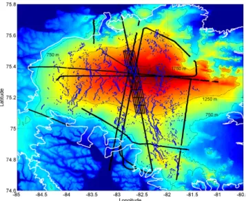
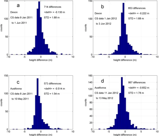
standard deviations of the differences were<15 cm. The po-sitions of the surface reference data and the centres of the CS2 footprints collected between January and May 2011 are illustrated in Fig. 3 by black and blue dots respectively. For each CS2 elevation the closest reference height was found. If the distance between the reference point and the centre of the CS2 footprint was less than 400 m, the height differ-ence was obtained and corrected for the slope between the two positions using the reference DEM. Although the CS2 data reflect a relatively large footprint (∼380 m along-track by∼100–1500 m across-track, dependent on slopes) in com-parison to the essentially point measurements from the refer-ence data set, the mean of over 700 height differrefer-ences (CS2 elevation minus the reference elevation) was−0.13 m with a standard deviation of 1.7 m (Fig. 4a). In spring 2012 NASA repeated some of the 2011 flight lines and a similar method-ology was used to compare the ATM laser elevations against the January to May 2012 CS2 elevations. In this case the mean height difference was−0.22 m with a similar standard
deviation (Fig. 4b). All of the CS2 data were acquired when the surface temperatures were below zero so we expect that, if calibrated correctly, the CS2 detected elevation would be lower than the actual surface elevation due to the expected volume component to the CS2 returns.
Similar results were obtained in the comparison of surface and CS2 elevations for Austfonna. Again, the surface refer-ence data were collected in the spring before any significant melt. Airborne laser (ALS) data were collected over Aust-fonna in spring 2011 and 2012, and surface kinematic GPS in every spring since CS2 was launched. Some of the results are summarized in Fig. 4c and d. The standard deviation of the CS2 minus surface elevation differences for the 2 years 2011 and 2012 were comparable to the results for Devon; 1.5 m (2011) and 1.8 m (2012), but the mean height differ-ences were larger;−0.51 m (2011) and−0.65 m (2012).
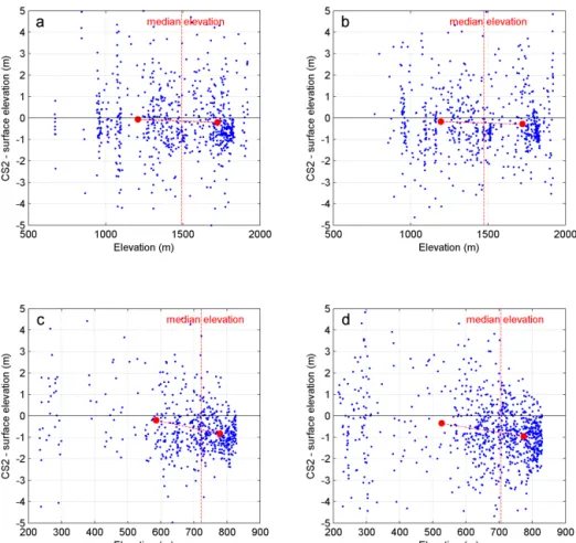
Figure 5 illustrates the individual bias points (CS2 – sur-face height) plotted against the elevation at which they were obtained. The median elevation for each data set is marked and the mean bias for elevations above and below the me-dian elevation are plotted with red markers. This shows that the bias between the surface and the CS2 elevation increases with elevation, particularly for Austfonna. In summary, under cold conditions any one CS2 elevation estimate will likely be lower than the surface elevation, but the bias between the surface and the CS2 elevation can be dependent on the con-ditions of the particular ice cap.
4.2 Error estimation
The average bias between the CS2 and surface elevations changed between 2011 and 2012 for both the Devon and Austfonna data sets. Are these changes from 2011 to 2012 (−0.13 to −0.22 m for Devon and −0.51 to −0.65 m for Austfonna) significant, or just a reflection of possible errors in the methodology? If each estimate is uncorrelated and part
Figure 3.Digital elevation model of Devon Ice cap showing the positions of the spring 2011 reference surface elevations (in black) and the CS2 elevations (in blue) acquired between 1 January and the end of May 2011. The rectangular grid over the ice cap sum-mit was collected from ground-based kinematic GPS surveys while the remaining transects were collected by ESA and NASA airborne missions. The white line indicates the approximate outer limit of glacial ice.
of a normal distribution, then the precision of the average can be estimated using the standard error of the mean; the stan-dard deviation of individual estimates divided by the square root of the number of estimates in the average. This leads to an estimate of∼0.06–0.07 m for the standard error of the means, implying that the year-to-year differences may be sig-nificant, and that there may have been some difference in the conditions year-to-year that led to the changing bias. How-ever, the histograms in Fig. 4 appear asymmetric so that the standard error may give an optimistic error estimate because the factors contributing to the spread in the results are not necessarily uncorrelated.
When we consider the errors in average height and height change we need to consider the following aspects:
1. Changes in near-surface physical characteristics: the CS2 signal will reflect from the surface if it is wet (e.g. summer), but can penetrate the surface if it is cold and dry (e.g. winter). Changing meteorological con-ditions; accumulation, storms, heavy snow falls, etc., could change the bias between the CS2 detected surface and the true surface, even during the winter. We expect that the magnitude of this variable bias may be depen-dent on the winter accumulation and the variability in conditions.
Figure 4.Histograms of the height differences, CS2 minus the reference elevations, acquired for Devon (a2011, andb2012) and Austfonna (c2011 andd2012). In the figures<delH>is the mean CS2 – reference elevation.
studied, some rapid changes, e.g. due to summer melt, may be poorly sampled. This error can be estimated for each location based on the slope of the summer height change and normally should be less than∼20 cm. 3. Spatial sampling – hypsometry: CS2 preferentially
sam-ples ridges and high areas since these are frequently the POCA position. Consequently, depressions and low-elevation regions will be undersampled. This can be cor-rected when a DEM is available because we know both the ice cap hypsometry and the distribution of elevations used for the CS2 average height change.
4. Spatial sampling – glacier facies: the height estimates may not uniformly sample the various glacier facies. As we cannot assume a constant bias between CS2 and the surface elevations for the different ice facies, the non-uniform sampling may lead to an additional error. These errors are difficult to quantify, but can be addressed on an ice-cap to ice-cap basis.
5. Altimetric corrections: there may be small systematic bias errors related to factors such as signal strength and surface slope, together with inaccuracies in atmospheric corrections.
The question remains; how well does the CS2 height change data reflect the surface height change? And what are the er-rors in any height change estimation? In general, these erer-rors have to be addressed on an ice-cap to ice-cap basis. The sam-pling errors, 2 to 4, will be greatest for the 30 day height changes due to the smaller sample sizes used, and should be small for year-to-year elevation change estimates when many thousands of points are averaged. Likewise, the noise and uncertainty in the CS2 results increases when analysing separate regions due to the use of fewer points than from the ice cap as a whole. When estimating year-to-year elevation change the error associated with a possible year-to-year bias change is likely less than the combined contributions of the temporal and spatial sampling for the 30 day data set that would occur by, for example, considering end of summer height from year-to-year.
unimpor-Figure 5. Biases between CS2 elevations and adjacent reference heights plotted against elevation for Devon (a2011 andb 2012) and Austfonna (c2011 andd2012). The red markers indicate the average biases above and below the median elevation.
tant as long as it has not changed in the time period between the two averages. The 0.09 and 0.14 m differences between the CS2 data and the reference data in 2011 and 2012 for De-von and Austfonna implies that this may happen, and that the possibility cannot be ignored.
5 Ice Cap results and discussion
In this section we present CS2 elevation results, first for De-von Ice Cap, using them to illustrate the elevation changes over time, and the correlation with independent surface ele-vation measurements and temperature data from sensors on an automatic weather station (AWS). Comparisons are also made with airborne Ku-band altimeter results. The same ap-proach is used when interpreting the height change data from the other ice caps.
5.1 Devon Ice Cap
We use∼60 000 CS2 elevation estimates over the Devon Ice Cap acquired from June 2010 to the end of December 2014 (Fig. 6). The separation into the NW (blue) and SE (maroon) sectors allows a comparison of regions with different average
accumulation. Although there are clear dips in the CS2 ele-vations during the two warm summers in 2011 and 2012, it is apparent that some of the CS2 elevation changes do not fol-low the AWS relative surface height change measurements during the cold winter–spring period (Fig. 7a and b). Indeed for the 2012–2013 winter the CS2 heights decrease from Oc-tober to April when, as shown by the height sensor, the sur-face height change should be relatively stable. While there is a slow downslope component of the AWS sensor movement, this explains just part of the discrepancy. Also, in February– March 2014 there is a dip in the CS2 derived height which is unlikely to be real.
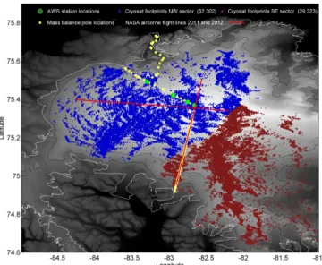
Figure 6.The coloured dots indicate the over 60 000 positions for which height data have been calculated superimposed on a grey scale representation of the Devon topography. Points for the NW and SE sectors are coloured dark blue and maroon respectively. The positions of the four automatic weather stations are indicated by the green dots and the mass balance pole positions are marked as yellow dots. Data from AWS “A” and “B” are included in Fig. 7. NASA acquired airborne Ku altimeter data (Fig. 8) over the flight lines marked in red in both 2011 and again in 2012.
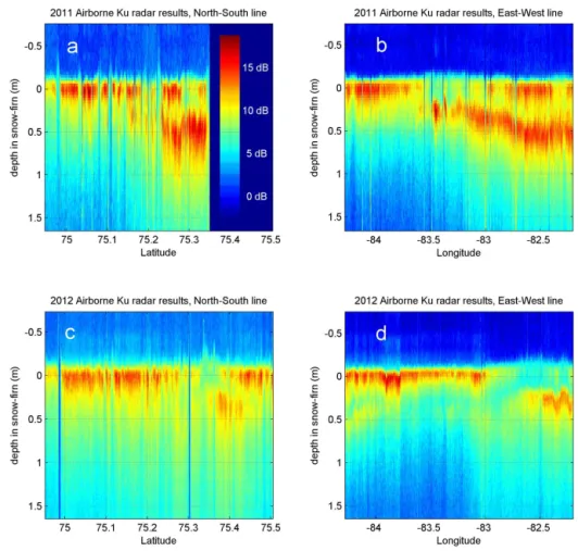
important to recognize that while the airborne altimeters can see subsurface layers it is very unlikely that the CS2 altimeter could resolve these features. The reason is not just the higher resolution of the airborne systems but rather the large differ-ence in the footprint size. In general, the shape of the leading edge of the CS2 return waveform is related to the time rate of change of illuminated area (controlled essentially by the topography), and the relative surface and volume backscat-ter. The link between the CS2 waveform shape and the ice cap topography was demonstrated by the success in simu-lating CS2 waveforms using only CS2 timing and position data, and the DEM produced by swath processing the CS2 data (Gray et al., 2013).
It is difficult to deconvolve the effect of surface topogra-phy and volume backscatter in traditional satellite altime-try data (Arthern et al., 2001), and the same is true for the delay-Doppler processed CS2 data. Consequently, the CS2 waveforms will be affected by the multiple layer and volume backscatter, but it is very unlikely that the CS2 could resolve the kind of layering that is visible in Fig. 8. It is possible that the changing nature of the winter accumulation reduces the surface reflectivity in relation to the volume component, such that the bias between the surface and the CS2 detected height increases during the winter. If the previous summer melt layer remains as the dominant backscatter layer then the apparent height could decrease because of firn compaction and the additional two-way path length due to the
permittiv-ity of the winter snow layer. This could then contribute to the apparent decrease in surface height seen in the 2012/13 win-ter.
The only time period when we can be confident that the peak return is simply related to the surface height is during the summer period when the solar illumination and above-zero surface temperatures lead to snow metamorphosis, a wet surface snow layer, densification and melt. With a wet sur-face layer the dominant returns will be from the sursur-face as losses increase for the component transmitted into the firn volume due to the presence of moisture.
Bearing this in mind, we can now begin to interpret the progression of CS2-derived elevation changes. In both 2011 and 2012 there was extensive summer melt across all ele-vations, accompanied by a clear CS2 height increase at the onset of melt (Fig. 7a). This apparent surface height increase likely reflects the transition from volume returns to a surface dominated return, rather than a real surface height increase. After the initial CS2 height increase, there was a clear de-crease in CS2 height throughout the rest of the summer, co-incident in time with melting temperatures and thus inter-preted as representing a real surface height decrease. This surface elevation decrease can therefore provide an estimate of summer ablation and snow/firn compaction. Following on from this, accumulation can then be estimated by differenc-ing the minimum height in one summer with the early sum-mer peak the following year, although this requires extensive melt across the ice cap for both summers, so would apply only for the winter 2011–12 accumulation on Devon Ice Cap. The influence of changing conditions on the apparent CS2-detected elevation was also observed with the low-resolution mode (LRM) data in Greenland after the extensive 2012 melt (Nilsson et al., 2015). In this work an apparent CS2 height in-crease was shown to be due to the creation of refrozen melt layers, and not a true surface height increase.
There is a marked contrast between the large CS2-derived height losses during the warm summers (June–August) of 2011 and 2012, compared to 2013, when there were low temperatures and little surface melt (Fig. 7c). How well the CS2 height changes represent summer melt can be assessed by comparison with the AWS and mass bal-ance pole data. From this it is clear that the maximum in accumulation and melt occur in the SE (Fig. 7a; ma-roon line vs blue line). Comparing the NW CS2 height changes with those measured at the lowest AWS, which at 1317 m is the closest to the average height of the NW sec-tor CS2 measurements, a good correspondence is found;
−0.72±0.5 m (CS2) vs. −0.64±0.03 m (AWS) for 2011, and −0.44±0.5 m (CS2) vs. −0.67±0.03 m (AWS) for 2012.
Figure 7. (a)Average CS2 height change over Devon Ice Cap as a function of time from July 2010 until December 2014 for all elevations (black), and for the NW (blue) and SE (maroon) sectors shown in Fig. 6. The short dashed black lines at the top indicate the time periods encompassing the CS2 passes which have been combined for the high temporal resolution plots. The four red dots indicate the winter-to-winter height change for all the elevation data for the time periods shown by the horizontal red lines.(b)Surface height change recorded by an ultrasonic surface height sensor on the AWS labelled A in Fig. 6. Black dots indicate the height change averaged over the same time frames as the CS2 winter-to-winter height change. The red dots show the same data corrected for the AWS vertical displacement.(c)Average AWS temperature data at the CS2 pass times (blue dots) and the cumulative positive degree day data (green).
the surface elevation change recorded at the AWS at 1317 m, averaged over the same period (Fig. 7b). However, because the AWS is fixed to the upper firn layers of the ice cap, it only provides a relative measure of surface height change. The red markers (Fig. 7b) indicate the AWS height change corrected for the −0.16±0.05 m a−1 vertical displacement
measured by GPS between spring 2013 and 2014, and with the same correction assumed for the other years. These ele-vation changes now show a better correspondence with the red markers in Fig. 7a.
The 3-year elevation change as a function of elevation (Fig. 9a) for Devon was obtained by differencing closely spaced elevation measurements from two time periods; the winter of 2013/14 minus elevations from the first winter of CS2 operation (2010/11). This indicates that surface eleva-tion decrease has been greatest at lower altitudes.
Table 1 includes the estimated accuracy of surface height change for the Devon Ice Cap based on CS2 measurements. The high temporal resolution row reflects the potential ac-curacy of year-to-year height change based on the monthly height estimates, and on the relative accuracy of monthly height change in the summer or winter. For Devon the errors include a possible bias change (item 1 in Sect. 4.2;∼0.2 m),
temporal and spatial sampling issues (items 2–4 in Sect. 4.2;
∼0.4 m) and the “altimetric” errors (item 5 in Sect. 4.2;
∼0.2 m). Assuming these contributions are independent, the root square sum will give the overall error but it should be emphasized that these results are rounded, and are estimates. The year-to-year height change (final row) is based on the much larger winter time periods and the sampling errors are much reduced.
5.2 Austfonna
Figure 8.Variability in surface and near-surface backscatter collected over Devon Ice Cap by the CReSIS Ku band altimeter in early May in both 2011(a, b)and 2012(c, d). The two left panels show the 2011 and 2012 reflected power as a function of penetration into the upper snow-firn layers and position along the north–south transect shown in Fig. 6. The two right panels show the change in return signal between the spring of 2011 and 2012 for the east–west line. A sub-surface propagation speed of 0.225 m ns−1was assumed in preparing this figure.
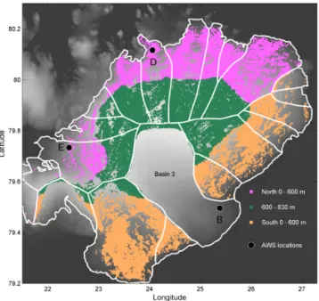
The CS2 elevation change for all three regions shows a clear drop during the summer melt period (Fig. 11a), and, as expected, is smaller for the high-elevation region. The largest summer height decreases were detected in 2013. This is in agreement with spring 2014 field observations indicat-ing very strong ablation durindicat-ing summer 2013, and is also re-flected in the air temperature recorded by the AWS station on Etonbreen (Fig. 11b). In comparing the CS2 and AWS sum-mer height loss data it appears that CS2 indicates less melt in the summer of 2012 than in 2011, but the three AWS surface height sensors show comparable melt. It should be noted that the positions and elevations of the AWS sensors (Fig. 10; Etonbreen, E; elevation 369 m, Duvebreen, D; 304 m and Basin 3, B; 175 m) may not be truly representative of the CS2 data. In particular, the average CS2 elevations for the low-elevation north and south data sets (459 and 380 m) are significantly higher than the relevant AWS elevations. Con-sequently, it is possible that the melt at higher elevations in 2012 was really less than that in 2011.
As discussed for the Devon Ice Cap, and expected from the ASIRAS results, the fluctuations in the high temporal
resolution CS2 height change data suggests that under cold conditions there can be a variable bias between the surface and CS2-derived heights. With the larger accumulation and milder, more variable winter temperatures on Austfonna one would expect the variable bias problem to be more severe than on Devon. For example, there is a large spike in ele-vation of 1 to 1.5 m between April and May 2013 for the southern low-elevation region (fawn in Figs. 10 and 11a). Data from the AWS in Basin-3 can be used to help explain this sudden jump; this indicates air temperatures in April of around−15◦C, before warm air moves in at the beginning
Figure 9.Height loss between the winter of 2010/11 and the winter of 2013/14 as a function of elevation for the five ice caps. Red lines are a linear fit to the data except for Austfonna(e)where the points are averages over 100 m elevation bands.
CS2 height in Table 1 has been estimated as 0.5 m, the same as for Devon.
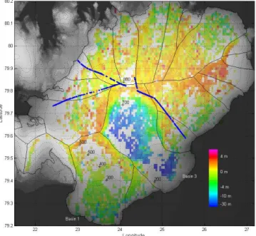
In the northern and summit region there is an over-all increase in average elevation over the CS2 time frame (Figs. 11a and 12). The total winter-to-winter elevation in-crease for the summit region is∼1 m over the 3 years from 2010/11 to 2013/14. This took place primarily in the first 2 years and there was little change in average high-altitude elevation between the winters of 2012/13 and 2013/14, span-ning the large melt in the summer of 2013 (Fig. 11a). The northern side shows a winter-to-winter increase in elevation for the first 2 years, which then dips to an overall increase in 3 years of∼0.5 m. This dip may also be related to the large 2013 melt. In contrast, the southern region has lost elevation. This may be explained partly by the hypsometry of Bråsvell-breen (Basin 1 in Fig. 12), a surge type glacier in its quiescent phase since the last surge in 1936/37. A large fraction of the glacier lies at low elevations, and is characterized by strong ablation.
We derived the height change over 3 years by taking all the height data from the last year of data acquisition, Novem-ber 2013 to DecemNovem-ber 2014, and subtracting the heights from July 2010 to December 2011 (Fig. 12). Individual pairs of height estimates within 400 m were differenced, slope cor-rected and binned into footprints of∼1 km2. The most
strik-Figure 10.The different basins on Austfonna are illustrated by the white lines. Data from Basin 3, which has surged during the CryoSat-2 time period, have been removed and studied separately. The remaining CS2 data set has been split into the areas shown in different colours above, and the temporal height change plotted for both a monthly and a winter-to-winter height change in Fig. 11 below. The positions of the three automatic weather stations are marked E, D and B.
Figure 11. (a)CS2 height change plots for the three different areas illustrated in different colours in Fig. 10. The square markers indicate the height change for the larger temporal winter-to-winter time periods (October to May). Sonic ranger heights and cumulative positive degree day (CPDD) data from the 3 AWS sensors are shown in(b).
approximation used for the others is not appropriate in this case.
5.3 Barnes Ice Cap
On Barnes Ice Cap the relative maximum power of each re-turn waveform shows increased power and dynamic range in the summers (Fig. 13a), which we interpret to be a conse-quence of significant melt and the possibility of a specular return from a wet surface. Initially moisture in the snow can reduce the backscatter but with continued melt and the cre-ation of a wet surface there is the possibility of relatively strong coherent reflection. The 30-day CS2 height changes (Fig. 13b) clearly show significant ice loss due to the warm summers in 2011 and 2012, with much lower losses in 2013 and 2014 due to the colder summers in those years.
Each year there is a small height increase in June, immedi-ately prior to the height loss due to summer melt (Fig. 13b). This is consistent with the observations for Devon and Aust-fonna, and is interpreted as the transition from a compos-ite surface and volume signal to one dominated by the snow surface as melt begins. The height loss due to summer melt each year ranged from 1.38 to 2.55 m, whereas winter
accu-mulation, estimated from the summer minimum in one year to the maximum at the onset of melt in the following year, remained relatively constant at∼1 m each winter. It is there-fore clear from the high temporal resolution data that summer melt is dominant in defining the annual mass balance. Esti-mating errors is more straightforward for Barnes because of the simpler configuration of surface facies: the ice cap con-sists essentially of snow over ice in winter, with the loss of all the winter snow the following summer. In this case we base the error estimate on the statistics of the 50+estimates of each height change: the error bars on the elevation change estimates (Fig. 13b) indicate±2 times the standard error of the mean. This approach has not been used for the other ice caps where it might lead to an optimistic error estimate (see Table 1). As the summer melt period has increased in recent years to∼87 days (Dupont et al., 2012) the potential error in summer height loss due to melt associated with the temporal sampling is also smaller than for Devon Ice Cap.
Figure 12.Three year height change estimates illustrated for differ-ent footprints across Austfonna. Each coloured pixel represdiffer-ents an average of the height change estimates in that footprint (∼1 km2). Note the colour scale is very nonlinear to better represent the height increase of a few metres at higher elevations, and in the northeast, and still illustrate the large height loss of∼30 m in the lower area in basin 3 due to the surge which began in 2012. The blue dots indi-cate the positions where surface elevation was measured with GPS in the spring of 2011 and again in 2014.
lost 2.75±0.2 m in average elevation, with most of that loss occurring in the summers of 2011 and 2012. These numbers agree well with the high temporal resolution height change estimates. An increase in melt at lower elevations on the ice cap is also observed (Fig. 9c), an effect originally shown by the work of Abdalati et al. (2004) and confirmed in the work of Gardner et al. (2012).
5.4 Agassiz and Penny ice caps
At 81◦N the Agassiz Ice Cap receives less accumulation and
has much less summer melt than the Penny Ice Cap on south-ern Baffin Island (67◦N). The magnitudes of the peak CS2
returns reflect these different surface temperature regimes: Agassiz experienced relatively less melt than Penny Ice Cap at high elevations even in the warm 2011 and 2012 sum-mers, consequently the seasonal variation in the peak returns is much less (Fig. 14a and b). The effect of summer melt on the CS2 returns is obvious in the Penny results (Fig. 14c and d). The strong peak returns even at high elevations at the end of July imply a strong specular reflection from a wet ice surface.
The increased time gap between the groups of passes evi-dent for Penny in comparison to those from Agassiz is due to the fact that the ascending and descending passes over Penny
occurred in the same time period, as well as the influence of the spreading of the passes due to the lower latitude.
There is little point in attempting to assess the monthly height change for either ice cap as there is simply not enough data (Table 1). However, winter-to-winter height change es-timates can be made on the assumption that the conditions have not changed between each winter so that the bias be-tween the physical surface and the CS2-detected elevation does not change. The average height change for the winters 2011/12, 2012/13 and 2013/14 with respect to the winter of 2010/11 show a larger ice loss for Penny Ice Cap in rela-tion to Agassiz (Fig. 14e). However, the ice loss on the two ice caps, Barnes and Penny, on Baffin Island is comparable. Again the effect of the warm 2011 and 2012 summers, and the contrast with the summer of 2013, is evident. On both ice caps, height loss decreases with increasing elevation (Fig. 9). The different climate regime between the Agassiz and Penny Ice Caps is obvious in the contrast between the plots of the peak returns in Fig. 14 (a, b vs. c, d). This implies that the bias between surface and CS2 detected surface will be less variable for Agassiz than Penny, and that the errors in surface height change will be smaller. This is reflected in the estimates of potential errors in the year-to-year height change (Table 1).
6 Conclusions
The airborne Ku band altimeter results over Devon Ice Cap and Austfonna imply that there will be a variable bias be-tween the physical surface and the heights derived from CryoSat-2. This has been confirmed with our analysis of CS2 data; with ice cap wide melt the bias between the mean de-tected CS2 elevation and the surface elevation will be a min-imum in the summer, but will increase with winter accumu-lation and the change in the nature of the surface. The tran-sition from freezing temperatures to melt in the early sum-mer is accompanied by an increase in the CS2 elevation, but without an equivalent increase in the surface height. This cor-responds to the transition from a composite surface-volume backscatter to one dominated by the surface. Under freezing conditions the bias between the CS2-derived elevation and the physical surface appears to vary with the current and his-torical conditions on the ice cap in a way that is hard to quan-tify although for Austfonna the difference appears to increase with increasing elevation.
Although some of the details of the seasonal change in el-evation, e.g. summer–winter, may change slightly with the form of the retracker, e.g. Ricker et al. (2015) showed some influence of the form of the retracker on sea ice freeboard results, we suspect that any CS2-detected elevation will be more dependent on the changing conditions than on the de-tailed form of the retracker.
Figure 13. (a)Maximum of each of the>44 000 waveforms from>300 CS2 passes over Barnes Ice Cap between 2010 and 2014. With extensive surface melt, both the dynamic range and average POCA power (dashed purple line) increase due to the occasional strong specular reflection;(b)height change over time based on the CS2 data grouped into 55 periods, which are shown as the short dashed lines in the upper part of the panel. Red dots and dotted line indicate the winter-to-winter height change calculated from the periods represented by the four red lines at the bottom of the panel.
Figure 14.Waveform maxima(a–d)for two elevation ranges of the Agassiz and Penny Ice Caps. The winter-to-winter average height change for the four data groups are shown with the same colours in(e).
change results can give a credible estimate of ice cap surface height change, particularly as more years are added to the time series. The largest uncertainty in these estimates, and the most difficult to quantify, comes from the fact that the conditions winter-to-winter may change in a manner that af-fects the bias between the surface and the CS2 elevation. Sur-face field measurements under cold spring conditions may help identify conditions which could lead to a changing bias between the CS2 and surface elevations. Hopefully, further work will improve the assessment of the efficacy and accu-racy of using CS2 heights to measure surface height change. The results for the Canadian ice caps show clearly the large year-to-year height decrease associated with the strong summer melt in 2011 and 2012. All show a net height loss over the CS2 time period, although Devon and Agassiz show a modest height increase after the low summer 2013 melt. This is in contrast to Austfonna where the summer of 2013 showed the largest melt-induced height loss although the up-per elevations of the ice cap appears to be still gaining ele-vation since mid-2010 when CryoSat-2 was commissioned. However, all the ice caps show a height loss at their lower elevations.
con-tinued loss of elevation even after the relatively cold snowy summer of 2013 attests to the eventual demise of this ice cap. In summary, we believe that the improved resolution and in-terferometric capability of the SARIn mode of Cryosat al-lows the user to identify the POCA position more accurately than with previous altimeters, and that the temporal height changes we have shown in this work depend to a large extent on the ability to better geocode the POCA footprint.
Acknowledgements. This work was supported by the European
Space Agency through the provision of CryoSat-2 data and the sup-port for the CryoVex airborne field campaigns in both the Canadian Arctic and Svalbard. NASA supported the IceBridge flights over the Canadian Arctic, while NSIDC and the University of Kansas (Cre-SIS) facilitated provision of the airborne laser and radar altimetry data. The Technical University of Denmark (TUD) managed the ESA supported flights over Devon and Austfonna. The IceBridge and TUD teams are gratefully acknowledged for the acquisition and provision of the airborne data used in this work. Processing of the ASIRAS instrument flown on the ESA CryoVex campaigns was done by the Alfred Wegener Institute, Bremerhaven. The Polar Con-tinental Shelf Project (Natural Resources Canada) provided logistic support for field work in the Canadian Arctic, and the Nunavut Re-search Institute and the communities of Grise Fjord and Resolute Bay gave permission to conduct research on the Agassiz and De-von ice caps. Support for D. Burgess and M. N. Demuth was pro-vided through the Climate Change Geoscience Program, Earth Sci-ences Sector, Natural Resources Canada and the GRIP programme of the Canadian Space Agency. Support for K. Langley was pro-vided by ESA project Glaciers-CCI (4000109873/14/I-NB). Wes-ley Van Wychen and Tyler de Jong helped with the 2011 kinematic GPS survey on Devon. NSERC funding to L. Copland is also grate-fully acknowledged.
We would like to thank V. Helm and the anonymous reviewer for the time and care they have taken with their reviews. Their comments have been very helpful and have improved the paper. Their contribution, and the help of the editor, E. Berthier, is gratefully acknowledged.
Edited by: E. Berthier
References
Abdalati, W., Krabill, F., Manizade, S., Martin, C., Sonntag, J., Swift, R., Thomas, R., Yungel, J., and Koerner, R.: Elevation changes of ice caps in the Canadian Arctic Archipelago, J. Geophys. Res.-Earth, 109, F04007, doi:10.1029/2003JF000045, 2004.
Abdalati, W., Zwally, H. J., Bindschadler, R., Csatho, B., Farrell, S. L., Fricker, H. A., Harding, D., Kwok, R., Lefsky, M., Markus, T., Marshak, A., Neumann, T., Palm, S., Schutz, B., Smith, B., Spinhirne, J., and Webb, C.: The ICESat-2 Laser Altimetry Mis-sion, Proc. IEEE, 98, 735–751, 2010.
Andrews, J. T. and Barnett, D. M.: Holocene (Neoglacial) moraine and proglacial lake chronology, Barnes Ice Cap, Canada, Boreas, 6, 341–358, 1979.
Arthern, R. J., Wingham, D. J., and Ridout, A. L.: Controls on ERS altimeter measurements over ice sheets: Footprint-scale to-pography, backscatter fluctuations, and the dependence of mi-crowave penetration on satellite orientation, J. Geophys. Res.-Atmos., 106, 33471–33484, doi:10.1029/2001JD000498, 2001. Baird, P. D.: Method of nourishment of the Barnes ice cap, J.
Glaciol., 2, 2–9, 1952.
Bamber, J., Krabill, W., Raper, V., and Dowdeswell, J.: Anomalous recent growth of part of a large Arctic ice cap: Austfonna, Svalbard, Geophys. Res. Lett., 31, L12402, doi:10.1029/2004GL019667, 2004.
Bell, C., Mair, D., Burgess, D., Sharp, M., Demuth, M., Cawkwell, F., Bingham, R., and Wadham, J.: Spatial and temporal variabil-ity in the snowpack of a High Arctic ice cap: implications for mass-change measurements, Ann. Glaciol., 48, 159–170, 2008. Bouzinac, C.: CryoSat-2 Product Handbook, Tech. Report,
Eu-ropean Space Agency, available at: http://emits.sso.esa.int/ emits-doc/ESRIN/7158/CryoSat-PHB-17apr2012.pdf (last ac-cess: 23 September 2015), 2014.
Brandt, O., Hawley, R. L., Kohler, J., Hagen, J. O., Morris, E. M., Dunse, T., Scott, J. B. T., and Eiken, T.: Comparison of airborne radar altimeter and ground-based Ku-band radar measurements on the ice cap Austfonna, Svalbard, The Cryosphere Discuss., 2, 777–810, doi:10.5194/tcd-2-777-2008, 2008.
Burgess, D. O.: Mass balance of the Devon (NW), Meighan, and South Melville ice caps, Queen Elizabeth Islands for the 2012–2013 balance year, Open File 7692, Geological Survey of Canada, Ottawa, Canada, p. 26, doi:10.4095/295443, 2014. Burgess, D. O., Sharp, M. J., Mair, D. W. F., Dowdeswell, J. A.,
and Benham T. J.: Flow dynamics and iceberg calving rates of the Devon Island ice cap, Nunavut, Canada, J. Glaciol., 51, 219– 238, doi:10.3189/172756505781829430, 2005.
Davis, C. H.: A robust threshold re-tracking algorithm for measuring ice-sheet surface elevation change from satellite radar altimeters, IEEE T. Geosci. Remote, 35, 974–979, doi:10.1109/36.602540, 1997.
Davis, C. H. and Segura, D. M.: An algorithm for time-series anal-ysis of ice sheet surface elevations from satellite altimetry, IEEE T. Geosci. Remote, 39, 202–206, 2001.
De la Pena, S., Nienow, P., Shepherd, A., Helm, V., Mair, D., Hanna, E., Huybrechts, P., Guo, Q., Cullen, R., and Wingham D.: Spa-tially extensive estimates of annual accumulation in the dry snow zone of the Greenland Ice Sheet determined from radar altimetry, The Cryosphere, 4, 467–474, doi:10.5194/tc-4-467-2010, 2010. Dowdeswell, J. A.: Drainage-basin characteristics of
Nordaust-landet ice caps, Svalbard, J. Glaciol., 32, 31–38, 1986.
Dowdeswell, J. A., Drewry, D., Cooper, A., Gorman, M., Liestøl, O., and Orheim, O.: Digital mapping of the Nordaustlandet ice caps from airborne geophysical investigations, Ann. Glaciol., 8, 51–58, 1986.
Dowdeswell, J. A., Benham, T. J., Strozzi, T., and Hagen, J. O.: Iceberg calving flux and mass balance of the Austfonna ice cap on Nordaustlandet, Svalbard, J. Geophys. Res., 113, F03022, doi:10.1029/2007JF000905, 2008.
Dunse, T., Schellenberger, T., Kääb, A., Hagen, J. O., Schuler, T. V. S., and Reijmer, C. H.: Glacier-surge mechanisms pro-moted by a hydro-thermodynamic feedback to summer melt, The Cryosphere, 9, 197–215, doi:10.5194/tc-9-197-2015, 2015. Dupont, F., Dupont, F., Royer, A., Langlois, A., Gressent, A., and
Picard, G.: Monitoring the melt season length of the Barnes Ice Cap over the 1979–2010 period using active and passive microwave remote sensing data, Hydrol. Process., 26, 2643, doi:10.1002/hyp.9382, 2012.
Ferguson, A. C., Davis, C. H., and Cavanagh, J. E.: An Autore-gressive Model for Analysis of Ice Sheet Elevation Change Time Series, IEEE. T. Geosci. Remote, 42, 2426–2436, 2004. Fisher, D. A., Koerner, R. M., Bourgeois, J. C., Zielinski, G., Wake,
C., Hammer, C. U., Clausen, H. B., Gundestrup, N., Johnsen, S., Goto-Azuma, K., Hondoh, T., Blake, E., and Gerasimoff, M.: Penny Ice Cap, Baffin Island, Canada and the Wisconsinan Foxe Dome connection: two states of Hudson Bay ice cover, Science, 279, 692–695, 1998.
Fisher, D. A., Zheng, J., Burgess, D. O., Zdanowicz, C., Kinnard, C., Sharp, M. J., and Bourgeois, J.: Recent melt rates of Canadian Arctic Ice Caps are the highest in many millennia, Global Planet. Change, 84/85, 3–7, doi:10.1016/j.gloplacha.2011.06.005, 2011. Galin, N., Wingham, D. J., Cullen, R., Fornari, M., Smith, W. H. F., and Abdall, S.: Calibration of the CryoSat-2 Interferometer and Measurement of Across-track Ocean Slope, IEEE T. Geosci. Remote., 51, 57–72, 2012.
Gardner, A. S., Moholdt, G., Wouters, B., Wolken, G. J., Burgess, D. O., Sharp, M. J., Cogley, J. G., Braun, C., and Labine, C.: Sharply increased mass loss from glaciers and ice caps in the Canadian Arctic Archipelago, Nature, 473, 357–360, doi:10.1038/nature10089, 2011.
Gardner, A. S., Moholdt, G., Arendt, A., and Wouters, B.: Acceler-ated contributions of Canada’s Baffin and Bylot Island glaciers to sea level rise over the past half century, The Cryosphere, 6, 1103–1125, doi:10.5194/tc-6-1103-2012, 2012.
Gardner, A. S., Moholdt, G., Cogley, J. G., Wouters, B., Arendt, A. A., Wahr, J., Berthier, E., Hock, R., Pfeffer, W. T., Kaser, G., Ligtenberg, S. R. M., Bolch, T., Sharp, M. J., Hagen, J. O., van den Broeke, M. R., and Paul, F.: A Reconciled Estimate of Glacier Contributions to Sea Level Rise: 2003 to 2009, Science, 340, 852–857, doi:10.1126/science.1234532, 2013.
Gray, L., Burgess, D., Copland, L., Cullen, R., Galin, N., Hawley, R., and Helm, V.: Interferometric swath processing of CryoSat-2 data for glacial ice topography, The Cryosphere, 7, 1857–1867, doi:10.5194/tc-7-1857-2013, 2013.
Hawley, R. L., Morris, E. M., Cullen, R., Nixdorf, U., Shepherd, A., and Wingham, D. J.: ASIRAS airborne radar resolves internal annual layers in the dry-snow of Greenland, Geophys. Res. Lett., 33, L04502, doi:10.1029/2005GL025147, 2006.
Hawley, R. L., Brandt, O., Dunse, T., Hagen, J. O., Helm, V., Kohler, J., Langley, K., Malnes, E., and Gda, K. H.: Using airborne Ku-band altimeter waveforms to investigate winter accumulation and glacier facies on Austfonna, Svalbard, J. Glaciol., 59, 893–899, 2013.
Helm, V., Rack, W., Cullen, R., Nienow, P., Mair, D., Parry, V., and Wingham, D. J.: Winter accumulation in the percolation zone of Greenland measured by airborne radar altimeter, Geophys. Res. Lett., 34, L06501, doi:10.1029/2006GL029185, 2007.
Helm, V., Humbert, A., and Miller, H.: Elevation and elevation change of Greenland and Antarctica derived from CryoSat-2, The Cryosphere, 8, 1539–1559, doi:10.5194/tc-8-1539-2014, 2014.
Jensen, J. R.: Angle measurement with a phase monopulse radar altimeter, IEEE T. Antenn. Propag., 47, 715–724, 1999. Koerner, R. M.: Accumulation on the Devon Island Ice Cap,
North-west Territories, Canada, J. Glaciol., 6, 383–392, 1966. Koerner, R. M.: Some observations on superimposition of ice on
the Devon Island Ice Cap, N.W.T., Canada, Geogr. Ann. A, 52, 57–67, 1970.
Koerner, R. M.: Mass balance of glaciers in the Queen Eliza-beth Islands, Nunavut, Canada, Ann. Glaciol., 42, 417–423, doi:10.3189/172756405781813122, 2005.
McMillan, M., Shepherd, A., Sundal, A., Briggs, K., Muir, A., Ridout, A., Hogg, A., and Wingham, D.: Increased ice losses from Antarctica detected by CryoSat-2, Geophys. Res. Lett., 41, 3899–3905, doi:10.1002/2014GL060111, 2014a.
McMillan, M., Shepherd, A., Gourmelen, N., Dehecq, A., Lee-son, A., Ridout, A., Flament, T., Hogg, A., Gilbert, L., Ben-ham, T., van den Broeke, M., Dowdeswell, J., Fettweis, X., Noël, B., and Strozzi, T.: Rapid dynamic activation of a marine-based Arctic ice cap, Geophys. Res. Lett., 41, 8902–8909, doi:10.1002/2014GL062255, 2014b.
Meier, M. F., Dyurgerov, M. B., Rick, U. K., O’Neel, S., Pfeffer, W. T., Anderson, R. S., Anderson, S. P., and Glazovsky, A. F.: Glaciers Dominate Eustatic Sea-Level Rise in the 21st Century, Science, 317, 1064–1067, doi:10.1126/science.1143906, 2007. Moholdt, G. and Kääb, A.: A new DEM of the Austfonna
ice cap by combining differential interferometry with ICESat laser altimetry, Polar Res., 31, 18460–18470, doi:10.3402/polar.v31i0.18460, 2012.
Moholdt, G., Hagen, J. O., Eiken, T., and Schuler, T. V.: Geometric changes and mass balance of the Austfonna ice cap, Svalbard, The Cryosphere, 4, 21–34, doi:10.5194/tc-4-21-2010, 2010. Nilsson, J., Vallelonga, P., Simonsen, S. B., Sørensen, L. S.,
Fors-berg, R., Dahl-Jensen, D., Hirabayashi, M., Goto-Azuma, K., Hvidberg, C. S., Kjær, H. A., and Satow, K.: Greenland 2012 melt event effects on CryoSat-2 radar altimetry, Geophys. Res. Lett., 42, 3919–3926, doi:10.1002/2015GL063296, 2015. Pinglot, J. F., Hagen, J. O., Melvold, K., Eiken, T., and Vincent, C.:
A mean net accumulation pattern derived from radioactive layers and radar soundings on Austfonna, Nordaustlandet, Svalbard, J. Glaciol., 47, 555–566, 2001.
Raney, R. K.: The Delay/Doppler Radar Altimeter, IEEE T. Geosci. Remote, 36, 1578–1588, 1998.
Ricker, R., Hendricks, S., Perovich, D. K., Helm, V., and Gerdes, R.: Impact of snow accumulation on CryoSat-2 range retrievals over Arctic sea ice: An observational approach with buoy data, Geo-phys. Res. Lett., 42, 4447–4455, doi:10.1002/2015GL064081, 2015.
Schuler, T. V., Dunse, T., Østby, T. I., and Hagen, J. O.: Meteoro-logical conditions on an Arctic ice cap – 8 years of automatic weather station data from Austfonna, Svalbard, Int. J. Climatol., 34, 2047–2058, doi:10.1002/joc.3821, 2014.
Sneed, W. A., Hooke, R. Le B., and Hamilton, G. S.: Thinning of the south dome of Barnes Ice Cap, Arctic Canada, over the past two decades, Geology, 36, 71–74, doi:10.1130/G24013A.1, 2008. Taurisano, A., Schuler, T. V., Hagen, J.-O., Eiken, T., Loe, E.,
Melvold, K., and Kohler, J.: The distribution of snow accumu-lation across Austfonna ice cap Svalbard: direct measurements and modeling, Polar Res., 26, 7–13, 2007.
VanWychen, W., Copland, L., Gray, L., Burgess, D., Danielson, B., and Sharp, M.: Spatial and temporal variation of ice motion and ice flux from Devon Ice Cap, Nunavut, Canada, J. Glaciol., 58, 657–664, doi:10.3189/2012JoG11J164, 2012.
Vaughan, D. G., Comiso, J. C., Allison, I., Carrasco, J., Kaser, G., Kwok, R., Mote, P., Murray, T., Paul, F., Ren, J., Rig-not, E., Solomina, O., Steffen, K., and Zhang, T.: Observations: Cryosphere, in: Climate Change 2013: The Physical Science Ba-sis, Contribution of Working Group I to the Fifth Assessment Report of the Intergovernmental Panel on Climate Change, Cam-bridge University Press, CamCam-bridge, UK and New York, NY, USA, 2013.
Wingham, D., Francis, C. R., Baker, S., Bouzinac, C., Cullen, R., de Chateau-Thierry, P., Laxon, S. W., Mallow, U., Mavrocordatos, C., Phalippou, L., Ratier, G., Rey, L., Rostan, F., Viau, P., and Wallis, D.: CryoSat-2: a mission to determine the fluctuations in earth’s land and marine ice fields, Adv. Space Res., 37, 841–871, 2006.