Adv. Sci. Res., 6, 227–231, 2011 www.adv-sci-res.net/6/227/2011/ doi:10.5194/asr-6-227-2011
©Author(s) 2011. CC Attribution 3.0 License.
Advances
in
Science & Research
Open Access Proceedings
EMS
Ann
ual
Meeting
and
8th
European
Conf
erence
on
Applied
Climatology
(ECA
C)
2010
Evaluating meteorological climate model inputs to
improve coastal hydrodynamic studies
D. Bellafiore1, E. Bucchignani2,3, S. Gualdi3, S. Carniel1, V. Djurdjeviæ4, and G. Umgiesser1,5
1ISMAR-CNR, Institute of Marine Science – National Research Council, Venice, Italy
2CIRA Italian Aerospace Research Centre, Capua, Italy
3
CMCC Centro Euro-Mediterraneo per i Cambiamenti Climatici, Bologna, Italy 4
SEE/VCCC – Institute of Meteorology, Faculty of Physics, University of Belgrade, Serbia 5
Coastal Research and Planning Institute (CORPI), Klaipeda University, Klaipeda, Lithuania
Received: 28 December 2010 – Revised: 19 July 2011 – Accepted: 8 August 2011 – Published: 22 August 2011
Abstract. This work compares meteorological results from different regional climate model (RCM) imple-mentations in the Mediterranean area, with a focus on the northern Adriatic Sea. The need to use these datasets as atmospheric forcings (wind and atmospheric pressure fields) for coastal hydrodynamic models to assess fu-ture changes in the coastal hydrodynamics, is the basis of the presented analysis. It would allow the assessment of uncertainties due to atmospheric forcings in providing coastal current, surge and wave climate changes from future implementations of hydrodynamic models.
Two regional climate models, with different spatial resolutions, downscaled from two different global climate models (whose atmospheric components are, respectively, ECHAM4 and ECHAM5), were considered. In particular, the RCM delivered wind and atmospheric pressure fields were compared with measurements at four stations along the Italian Adriatic coast. The analyses were conducted using a past control period, 1960–1990, and the A1B IPCC future scenario (2070–2100). The chosen scenario corresponds to a world of very rapid economic and demographic growth that peaks in mid-century, with a rapid introduction of new efficient tech-nologies, which balance fossil and non-fossil resources (IPCC, 2007). Consideration is given to the accuracy of each model at reproducing the basic statistics and the trends. The role of models’ spatial resolution in reproducing global and local scale meteorological processes is also discussed. The Adriatic Sea climate is affected by the orography that produces a strengthening of north-eastern katabatic winds like bora. Therefore, spatial model resolution, both for orography and for a better resolution of coastline (Cavaleri et al., 2010), is one of the important factors in providing more realistic wind forcings for future hydrodynamic models im-plementations. However, also the characteristics in RCM setup and parameterization can explain differences between the datasets. The analysis from an ensemble of model implementation would provide more robust indications on climatic wind and atmospheric pressure variations. The scenario-control comparison shows a general increase in the mean atmospheric pressure values while a decrease in mean wind speed and in extreme wind events is seen, particularly for the datasets with higher spatial resolution.
1 Introduction
One of the major aspects discussed in recent works on cli-mate changes is how to provide information from the global scale to the local one. In fact, the impacts that sea level rise and changes in the meteorological conditions due to climate changes might have on the coastal zone are relevant for
mit-Correspondence to:D. Bellafiore ([email protected])
228 D. Bellafiore et al.: Evaluating meteorological climate model inputs
Table 1.Summary table of the five analyzed RCM datasets.
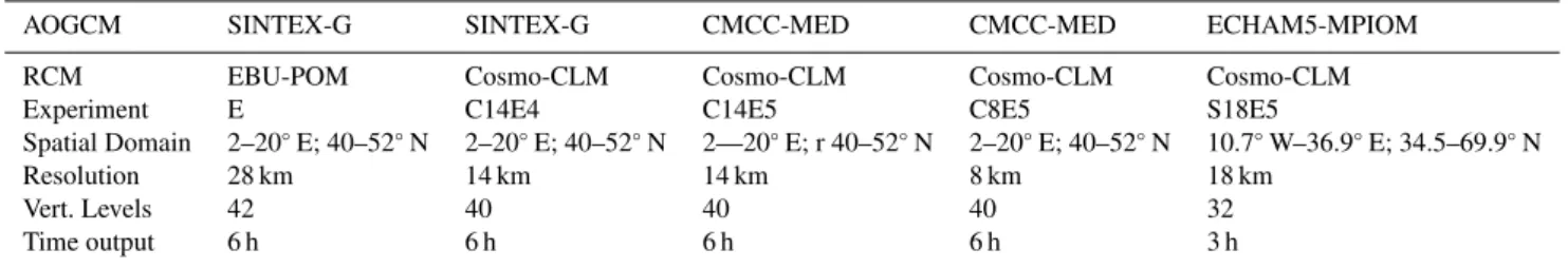
AOGCM SINTEX-G SINTEX-G CMCC-MED CMCC-MED ECHAM5-MPIOM
RCM EBU-POM Cosmo-CLM Cosmo-CLM Cosmo-CLM Cosmo-CLM
Experiment E C14E4 C14E5 C8E5 S18E5
Spatial Domain 2–20◦E; 40–52◦N 2–20◦E; 40–52◦N 2—20◦E; r 40–52◦N 2–20◦E; 40–52◦N 10.7◦W–36.9◦E; 34.5–69.9◦N
Resolution 28 km 14 km 14 km 8 km 18 km
Vert. Levels 42 40 40 40 32
Time output 6 h 6 h 6 h 6 h 3 h
there is only one attempt to verify the capability to reproduce wind fields and, therefore, storminess induced in the coastal zone (Woth et al., 2006). The wind driver, compared with other variables analyzed in climate change studies, such as temperature, has the peculiarity to be highly spatially vary-ing and strongly characterized on small scales. The chal-lenge is to quantify climatic effects due to wind on the local scale. The capability to reproduce storminess is fundamen-tal for local coasfundamen-tal management, in order to deal with the main threats of these areas, like coastal floodings and severe erosion events.
2 Methods
2.1 Climate models description and setup
Datasets from the different RCMs were analyzed comparing wind and atmospheric pressure fields both for the control pe-riod (1960–1990) and the IPCC A1B scenario (2070–2100). Regional models consider limited domains, therefore boundary conditions are obtained from global climate simu-lations. Results are provided for the control period (1960– 1990) and for the A1B IPCC scenario (2070–2100). The considered datasets are summarized in Table 1, defining the atmospheric-ocean global climate models (AOGCM) that provide initial and boundary conditions, besides time step, spatial domain and resolution of the RCMs.
The AOGCM SINTEX-G is a coupled atmosphere-ocean general circulation model, whose atmospheric component is ECHAM4 (Roeckner et al., 1996). The ocean model com-ponent is the reference version 8.2 of the Ocean Parallelise (OPA; Madec et al., 1999) with the ORCA2 configuration. The AOGCM CMCC-MED is formed by the atmospheric model ECHAM5 (Roeckner et al., 2003) and the global ocean component OPA in the ORCA2 configuration. In the Mediterranean region, CMCC-MED uses a high-resolution model of the Mediterranean Sea (NEMO-MFS, Oddo et al., 2009) able to resolve the small scale dynamics of the basin.
ECHAM4 has ∼120 km (T106) spatial resolution, 12 h time resolution and runs on 360 days yearly, while ECHAM5 spatial resolution is∼80 km (T159), 6 h time resolution and runs on 365 days yearly.
The coupled global model where the S18E5 RCM is nested to is ECHAM5-MPIOM (MPIOM is the ocean model of the Max Planck Inst. Germany).
The first RCM is EBU-POM (Eta Belgrade University – Princeton Ocean Model), a coupled regional climate model that is the combination of two limited area models one for the atmosphere and the other for the ocean (Djurdjevic and Rajkovic, 2008, 2010; Gualdi et al., 2008). The atmospheric component is the Eta/NCEP (National Centers for Environ-mental Prediction) limited area model, which is a hydrostatic primitive equation, grid-point model (Janjic, 1984; Mesinger et al., 1988).
The second RCM is COSMO-CLM (Rockel et al., 2008), the climate version of the COSMO model, which is the op-erational non-hydrostatic mesoscale weather forecast model developed by the German Weather Service (DWD).
EBU-POM (hereafter called dataset E) has initial and boundary conditions taken from SINTEX-G. Simulated years are of 360 days, as in the global model.
The COSMO-CLM model was used to generate four dif-ferent datasets. Three of them were produced at the Ital-ian Aerospace Research Centre (CIRA), one forced by the AOGCM SINTEX-G (C14E4), and two (C14E5 and C8E5) by the AOGCM CMCC-MED. The fourth (S18E5) was gen-erated at the DWD and forced by the AOGCM ECHAM5-MPIOM. The latter model implementation introduces a sub-stantial smoothing of the Caucasus Mountains orography to the constant height of 150 m, which is the mean height in the ECHAM5-MPIOM model for that region.
The meteorological fields from models are bilinearly in-terpolated on a finite element grid to extract wind and at-mospheric pressure time series in the meteorological stations presented in the next section.
2.2 Measurements
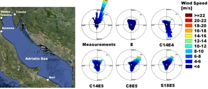
Figure 1.Location of wind stations (left panel). In the right panels, the wind direction distribution (direction of provenience) for E, C14E4, C14E5, C8E5, S18E5 and the measured datasets for the Trieste Station are shown for the reference period (1960–1990).
observational data sets are compared with the model simula-tions for the period 1960–1990, that we will refer to as the reference period. Data are provided every 3 h.
3 Results and discussion
3.1 Reference period
A preliminary analysis has been carried out to evaluate the ef-fects related to the increase in the spatial resolution of RCMs, and the influence of the boundary conditions obtained from the different global models in reproducing wind and atmo-spheric pressure statistics for the reference period.
The modeled and measured mean wind speed and atmo-spheric pressure values are compared for the selected stations (Fig. 1, left panel). The mean wind speed in Venice Tessera is better reproduced by dataset E than by the others, though underestimated (−11 %). On the other hand, the high res-olution COSMO-CLM datasets (C14E4, C8E5, S18E5) are not able to reproduce the wind speed statistics in the north-western Adriatic. In particular, they appear to overestimate the wind speed by about 40 %. Interestingly, these models appear to perform better when compared with the other sta-tions (e.g., Ravenna and Bari). This aspect can be explained observing that these latter stations are less characterized by specific wind regimes, also due to the lack of orographic ef-fects. Therefore the models encounter less criticities linked with spatial resolution. Considering the two datasets C14E5 and C8E5, both laterally forced by ECHAM5 global cli-mate model but running with different spatial resolutions, the lower resolution (C14E5) seems to be in better agree-ment with observations, especially in terms of mean wind speed. The C14E5 results appear to be remarkably good for
the Ravenna station case, where the C8E5 dataset exhibits an overestimation of the wind speed of about 29 %. This suggests that a simple increase of the resolution does not automatically improve the results, at least in terms of mean wind field. Resolution, in any case, plays an important role in defining the correct wind regimes and, particularly in Trieste, the wind directions are fairly matched by C8E5 than C14E5 (Fig. 1, right panel) . On the other hand, resolution is not the only changing aspect between the different datasets, since different setups are used for the COSMO-CLM simulations performed at the CIRA Institute (C14E4, C14E5, C8E5) and for the one provided by the World Data Center for Climate (S18E5). In the latter case, a smoothing of the Balkan orog-raphy was performed to avoid numerical errors, even if this has led to a less realistic representation of the mountains in the region. However, despite the approximation, the model appears to perform better than the others in reproducing kata-batic winds as bora in the Adriatic Sea area. A comparison with the Trieste station, in fact, indicates that S18E5 pro-vides better results both in terms of extreme events (−0.7 % compared to higher underestimation obtained with the other models) and in the wind direction (Fig. 1, right panel). Gen-erally, the majority of models miss the dominant NNE wind direction, probably due to the need of increased resolution and a proper dealing of orography reproduction to simulate this wind regime.
230 D. Bellafiore et al.: Evaluating meteorological climate model inputs
Table 2. Differences between A1B scenario (2070–2100) and reference period (1960–1990)−100 (A1B−reference)/reference−for mean and 99th percentile values of atmospheric pressure (left panel) and wind speed (right panel).
Mean Atmospheric Pressure [%] Mean Wind Speed [%]
Stations E C14E4 C14E5 C8E5 S18E5 E C14E4 C14E5 C8E5 S18E5
VeT 0.00 0.02 0.06 0.06 0.23 −7.91 −6.26 −4.32 −5.31 −4.68 Ts 0.01 0.03 0.07 0.06 0.24 −5.33 −6.71 −0.52 −4.49 −4.57 Ra 0.01 0.03 0.07 0.06 0.24 −5.52 −5.01 −0.43 −4.00 −3.19 Ba 0.01 0.03 0.07 0.06 0.24 −5.24 −7.65 −0.91 −4.19 −5.08
Atmospheric Pressure 1st percentile [%] Wind Speed 99th percentile [%]
Stations E C14E4 C14E5 C8E5 S18E5 E C14E4 C14E5 C8E5 S18E5
VeT 0.07 0.11 0.16 0.16 0.30 −5.01 −3.93 −4.43 −4.55 −0.11
Ts 0.11 0.06 0.07 0.02 0.27 −9.26 −6.07 −2.69 −3.65 −2.18 Ra 0.11 0.05 0.07 0.03 0.29 −9.69 −4.89 −1.83 −3.97 −3.41 Ba 0.11 0.06 0.07 0.03 0.27 −9.70 −6.09 −2.64 −1.74 −1.64
The computation of extremes (99th percentiles for wind speed and 1st percentile for atmospheric pressure outputs), allows the evaluation of the model performance under ex-treme wind events. The best performances for atmospheric pressure are given by the high resolution models downscaled from ECHAM5 (C14E5, C8E5, overestimation∼+0.5 % as an average). Wind speed extremes are better reproduced by C14E5 (underestimation ∼+5 % as an average). This would suggest an influence of AOGCM, where the ECHAM5 that seems to have more realistic characteristics compared to ECHAM4 performs better (increased resolution, different se-tups, etc.). On the other hand, the reduced Balkan orography introduced in the S18E5 can explain the underestimation of 99th percentile values of wind speed in the North Adriatic stations by this dataset.
3.2 A1B scenario comparison
The study of meteorological outputs for each model allows the definition of variations in the future scenarios. Analyz-ing the mean wind speed variations in the future A1B IPCC scenario, compared with the reference period, it is evident that the majority of models simulate a general decrease in the four coastal stations, higher for models downscaled from ECHAM4 (E and C14E4 dataset, Table 2). Considering the mean atmospheric pressure variations, the strongest increase is registered by the S18E5 (see again Table 2). A strong decrease in the wind extreme values is depicted by the E and C14E4 datasets (∼−9 % and∼−6 %, Table 2), while the other datasets register smaller decreases. However all sta-tions identify the same tendency. On the other hand, the anal-ysis of the 1st percentile for the atmospheric pressure shows a slight increase in the extreme low pressure values, ten-dency confirmed by all models. Performing a Kolmogorov-Smirnov hypothesis test, for each station on the control pe-riod and A1B scenario wind and atmospheric pressure time
series, where p-values are almost 0 everywhere, what arises is that differences in mean and distribution between them are significant.
4 Conclusions
The outcomes of this preliminary work on the Adriatic Sea highlight uncertainties intrinsic in the dynamical downscaling approach from GCM simulations to spatial scales suitable to study climate change impacts on coastal dynamics at the local scale. Despite the limitation and the still preliminary phase of the work, we think this analysis has pointed out the main problems in bridging the gap between the coarse information provided by the climate simulations and the detailed information required to investigate the climate change impacts and risks at the local level: increased resolution may not improve the models’ reproduction of certain variables (i.e. atmospheric pressure) and the global model choice and setup could impact models’ outputs. The different skills shown by the models in reproducing wind and atmospheric pressure fields suggest that ensemble of simulations would probably provide more robust climatic forcings for coastal hydrodynamic modeling implementa-tions.
Acknowledgements. The support of the European Commission
through FP7.2009-1, Contract 244104-THESEUS (“Innovative technologies for safer European coasts in a changing climate”) is gratefully acknowledged. The authors want to thank the World Data Center for Climate for the provision of the S18E5 dataset. Thanks also to B. Rajkovic for producing the E dataset and E. Scoccimarro for the help in handling the E dataset.
Edited by: W. May
The publication of this article is sponsored by the Swiss Academy of Sciences.
References
Cavaleri, L., Bertotti, L., Buizza, R., Buzzi, A., Masato, V., Umgiesser, G., and Zampieri, M.: Predictability of extreme meteo-oceanographic events in the Adriatic Sea, Q. J. Roy. Me-teor. Soc., 136, 400–413, 2010.
Djurdjevic, V. and Rajkovic, B.: Verification of a cou-pled atmosphere-ocean model using satellite observations over the Adriatic Sea, Ann. Geophys., 26, 1935–1954, doi:10.5194/angeo-26-1935-2008, 2008.
Djurdjevic, V. and Rajkovic, B.: Development of the EBU-POM coupled regional climate model and results from climate change experiments, in: Advances in Environmental Modeling and Mea-surements, edited by: Mihajlovic, T. D. and Lalic, B., Nova Pub-lishers, 2010.
Giorgi, F., Bi, X., and Pal, J. S.: Mean. interannual variability and trends in a regional climate change experiment over Europe, Clim. Dynam., 22, 733–756, doi:10.1007/s00382-004-0409-x, 2004.
Gualdi, S., Rajkovic, B., Djudjevic, V., Castellari, S., Scocci-marro, E., Navarra, A., and Dadic, M.: Simulation of climate change in the mediterranean area, Web, Final Scientific, http:
//www.earth-prints.org/bitstream/2122/4675/1/SINTA FInal% 20Science%20Report%20 October%202008.pdf, 2008. IPCC: Climate Change 2007, Synthesis Report, Technical report,
IPCC-Intergovernamental Panel for Climate Change, 2007. Janjic, Z.: Non-linear advection schemes and energy cascade on
semi staggered grids, Mon. Weather Rev., 112, 1234–1245, 1984.
Madec, G., Delecluse, P., Imbard, M., and Levy, C.: OPA 8.1 Ocean General Circulation Model reference manual, Internal Rep. 11, Inst. Pierre-Simon Laplace, Paris, France, 1999.
Mesinger, F., Janjic, Z., Nicovic, S., Gavrilov, D., and Daven, D.: The step mountain coordinate: model description and perfor-mance for cases of alpine lee cyclogenesis and for a case of an Appalachian redevelopment, Mon. Weather Rev., 116, 1493– 1518, 1988.
Oddo, P., Adani, M., Pinardi, N., Fratianni, C., Tonani, M., and Pet-tenuzzo, D.: A nested Atlantic-Mediterranean Sea general circu-lation model for operational forecasting, Ocean Sci., 5, 461–473, doi:10.5194/os-5-461-2009, 2009.
Rockel, B., Will, A., and Hense, A.: The regional Climate Model COSMO-CLM (CCLM), Meteorol. Z., 17(4), 347–348, 2008. Roeckner, E., Arpe, K., Bengtsson, L., Christoph, M., Claussen,
M., D¨umenil, L., Esch, M., Giorgetta, M., Schlese, U., and Schulzweida U.: The atmospheric general circulation model ECHAM-4: Model description and simulation of present-day cli-mate, Max Planck Institut fur Meteorologie, report 218, 90 pp., 1996.
Roeckner, E., B¨auml, G., Bonaventura, L., Brokopf, R., Esch, M., Giorgetta, M., Hagemann, S., Kirchner, I., Kornblueh, L., Manzini, E., Rhodin, A., Schlese, U., Schulzweida, U., and Tompkins, A.: The atmospheric general circulation model ECHAM 5, Max-Planck-Institut fuer Meteorologie, report 349, Hamburg, 140 pp., ISSN 0937-1060, 2003.
Woth, K., Weisse, R., and Von Storch, H.: Climate change and North Sea storm surge extremes: an ensemble study of storm surge extremes expected in a changed climate projected by four different regional climate models, Ocean Dynam., 56, 3–15, doi:10.1007/s10236-005-0024-3, 2006.