Model of optical response of marine aerosols to Forbush decreases

(1)

ACPD

9, 22833–22863, 2009

Model of optical response of marine aerosols to Forbush

decreases

T. Bondo et al.

Title Page

Abstract Introduction

Conclusions References

Tables Figures

◭ ◮

Back Close

Full Screen / Esc

Printer-friendly Version

Interactive Discussion

Atmos. Chem. Phys. Discuss., 9, 22833–22863, 2009 www.atmos-chem-phys-discuss.net/9/22833/2009/ © Author(s) 2009. This work is distributed under the Creative Commons Attribution 3.0 License.

Atmospheric Chemistry and Physics Discussions

This discussion paper is/has been under review for the journalAtmospheric Chemistry

and Physics (ACP). Please refer to the corresponding final paper inACPif available.

Model of optical response of marine

aerosols to Forbush decreases

T. Bondo, M. B. Enghoff, and H. Svensmark

National Space Institute, Technical University of Denmark, Copenhagen, Denmark

Received: 18 August 2009 – Accepted: 1 October 2009 – Published: 27 October 2009

Correspondence to: T. Bondo ([email protected])

(2)

ACPD

9, 22833–22863, 2009

decreases

T. Bondo et al.

Title Page

Tables Figures

◭ ◮

Back Close

Full Screen / Esc

Abstract

In order to elucidate the effect of galactic cosmic rays on cloud formation, we

investi-gate the optical response of marine aerosols to Forbush decreases – abrupt decreases in galactic cosmic rays – by means of modeling. We vary the nucleation rate of new aerosols, in a sectional coagulation and condensation model, according to changes in

5

ionization by the Forbush decrease. From the resulting size distribution we then cal-culate the aerosol optical thickness and Angstrom exponent, for the wavelength pairs 350, 450 nm and 550, 900 nm. For the shorter wavelength pair we observe a change

in Angstrom exponent, following the Forbush Decrease, of−6 to+3% in the cases with

atmospherically realistic output parameters. For some parameters we also observe

10

a delay in the change of Angstrom exponent, compared to the maximum of the

For-bush decrease, which is caused by different sensitivities of the probing wavelengths to

changes in aerosol number concentration and size. For the long wavelengths these changes are generally smaller. The types and magnitude of change is investigated for a suite of nucleation rates, condensable gas production rates, and aerosol loss rates.

15

Furthermore we compare the model output with observations of 5 of the largest For-bush decreases after year 2000. For the 350, 450 nm pair we use AERONET data and find a comparable change in signal while the Angstrom Exponent is lower in the model than in the data, due to AERONET being mainly sampled over land. For 550, 900 nm we compare with both AERONET and MODIS and find little to no response in

20

both model and observations. In summary our study shows that the optical properties of aerosols show a distinct response to Forbush Decreases, assuming that the nucle-ation of fresh aerosols is driven by ions. Shorter wavelengths seem more favorable for

observing these effects and great care should be taken when analyzing observations,

in order to avoid the signal being drowned out by noise.

(3)

ACPD

9, 22833–22863, 2009

decreases

T. Bondo et al.

Title Page

Tables Figures

◭ ◮

Back Close

Full Screen / Esc

1 Introduction

A Forbush Decrease (FD) is a sudden drop in the amount of galactic cosmic rays observed on Earth, due to large Coronal Mass Ejections from the sun (Forbush, 1937; Cane, 2000). The largest of these events cause up to 10–25% changes in the cosmic ray count rate but occur rarely – only about once a year – and typically last from a few

5

days to about a week. A correlation between galactic cosmic rays (controlled by solar activity) and cloud cover has been shown (Marsh and Svensmark, 2003; Harrison and Stephenson, 2006). If this correlation is due to a physical mechanism a response in cloud cover could be expected during or after a Forbush decrease. An investigation of a connection between clouds and cosmic rays on a FD time scale would also be able to

10

narrow down the number of potential explanations for the cloud – cosmic ray connection as no solar parameters (such as total solar irradiance) correlate well with FD Neutron

Monitor counts during the span of a Forbush decrease. FD effects in cloud data have

been investigated previously (Pudovkin and Veretenenko, 1995; Kniveton, 2004; Todd and Kniveton, 2004; Harrison and Stephenson, 2006; Kristj ´ansson et al., 2008; Sloan

15

and Wolfendale, 2008; Svensmark et al., 2009) but no definitive conclusion has been reached. Pudovkin and Veretenenko (1995) investigated 65 Forbush decreases from 1969 to 1986 over four latitudinal bands in Russia and found a significant response in

cloud cover in the 60–64◦ band. Todd and Kniveton (2004) found a decrease in high

cloud cover over Antarctica, using ISCCP D1 data from 1983 to 2000. They conclude

20

that their result could just as well be due to the uncertainties in polar cloud retrieval as

it could be a real signal. Correlations at 20–30◦N and 10–20◦S also appear when the

effects of rainfall are removed (Kniveton, 2004). In Harrison and Stephenson (2006),

ground level observations of the diffuse fraction of light due to scattering by particles

are found to be affected by Forbush decreases in the period 1968 to 1994. In Tinsley

25

(4)

ACPD

9, 22833–22863, 2009

decreases

T. Bondo et al.

Title Page

Tables Figures

◭ ◮

Back Close

Full Screen / Esc

ocean regions. Little significant response in cloud parameters was found even though the correlations improved somewhat by focusing on the six strongest events. Sloan and Wolfendale (2008) found no significant response either. This is in contrast to results from Svensmark et al. (2009) where an epoch analysis of three independent data sets was used to show a decrease in liquid water clouds about 10 days after a FD. These

5

results are explained as a decrease in nucleation mode aerosols growing to affect CCN

and cloud cover over a time period similar to the 10 day lag.

Another approach to this issue is to calculate whether it would be plausible to ex-pect a signal at all. Clouds are formed on aerosols and it has been indicated by theory (Arnold, 1980; Laakso et al., 2002; Lovejoy et al., 2004; Yu, 2006),

observa-10

tions (Eichkorn et al., 2002; Lee et al., 2003; Hirsikko et al., 2007; Laakso et al., 2007;

Kulmala et al., 2007) and experiments (Kim et al., 1997; Enghoffet al., 2008; Winkler

et al., 2008) that ions, formed by cosmic rays, can enhance the formation of these par-ticles. Therefore it can be expected that if a signal in cloud cover, following a Forbush decrease, is to be found, there should also be a signal in the aerosols.

15

Motivated by the findings in Svensmark et al. (2009) we try to model how such a response would appear in the aerosol optical properties under the assumption that the cluster formation has been modified by the ionization change during the FD. Two pa-rameters are used to describe the optical properties of aerosol populations: Aerosol Optical Thickness (AOT) and the Angstrom exponent (AE). The AOT is being

mea-20

sured routinely throughout the atmosphere by photometers such as it is being done by AERONET (Holben et al., 1998) – a network of aerosol observations covering most of Earth. It is a measure for how much light penetrates the atmosphere at a given wavelength, such that a higher AOT means that less light gets through. Both particle

number concentration and radius affects the AOT thus changes in AOT can be

inter-25

preted in various ways. The AE (Schuster et al., 2006) is the slope of the line in a

log (AOT) vs log (λ) plot, whereλis the wavelength. Since the AOT at a givenλis more

sensitive to particles that are close toλin size the AE holds information about the size

(5)

ACPD

9, 22833–22863, 2009

decreases

T. Bondo et al.

Title Page

Tables Figures

◭ ◮

Back Close

Full Screen / Esc

is the existing population of primary aerosols, from pollution, dust storms, sea spray etc. These large particles, which are produced regardless of cosmic rays, is a major sink to freshly nucleated particles (Pierce and Adams, 2007) and can potentially drown out any signal in the aerosol distribution from Forbush decreases. Two recent model

papers arrive at di_fferent conclusions on the probability of formation of CCN from

ultra-5

fine condensation nuclei (Kuang et al., 2009; Pierce and Adams, 2009) which will affect

the signal following a FD. This underlines the relevance of further studies on aerosol growth.

We use a basic nucleation and growth model, sensitive to the cosmic ray flux, to simulate the evolution of a particle distribution in marine conditions, during a Forbush

10

event. In order to calculate the optical properties of the particle distribution the growth model is coupled to a Mie Scattering program: Miex (Wolf, 2004). The sea salt op-tical properties are derived from the opop-tical properties program OPAC (Hess et al., 1998). Finally we compare the modeling results with measurements from AERONET and MODIS (Platnick et al., 2003).

15

2 Theoretical model

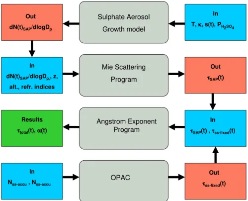
We are interested in determining the changes in the optical properties of a cloud-free marine environment consisting of sulphur gases and sea salt during a Forbush decrease. The theoretical approach is based on 4 steps as illustrated in Fig. 1 and outlined below.

20

– Aerosol growth model: neutral sulphuric acid aerosol growth is simulated in a

marine environment where the cluster production is modulated during a FD. In this part three parameters are varied: the gas phase sulphuric acid production rate, the particle loss rate, and the production rate of stable sulphuric acid clusters.

– Miex part: the particle distribution as a function of time is input to a Mie Scattering

25

(6)

ACPD

9, 22833–22863, 2009

decreases

T. Bondo et al.

Title Page

Tables Figures

◭ ◮

Back Close

Full Screen / Esc

the extinction coefficients and optical depths.

– OPAC part: simultaneously, an optical properties program (OPAC) is used to

cal-culate the optical depth of a fixed sea salt distribution representative for the marine troposphere.

– Optical properties: finally, the total optical depth and Angstrom exponent is

cal-5

culated as a function of time for the combined sea salt distribution and sulphuric acid particles.

2.1 The aerosol growth model

The numerical model is based on the general dynamic equation (GDE) which is a

par-tial differential equation for aerosol particle growth (Seinfeld and Pandis, 2006). A

sec-10

tional method is used to solve the GDE to determine the number distributionn, where

bins of variable sizes represent different sizes of the molecular clusters expressed as

the number of sulphuric acid molecules in the cluster. The sizes of these bins can be chosen arbitrarily but can limit the integration accuracy. In this work the initial clusters are sampled with each bin representing the addition of one sulphuric acid molecule

15

up to 70 molecules (approx. 3.5 nm) followed by a slowly increasing bin size to around 450 molecules and then the bin size is increased with a factor of 1.1 per bin.

The model includes the production and loss of particles by condensation of sulphuric acid gas onto particles and the coagulation of the individual particle clusters but

evap-oration is not considered. The condensation coefficients k_ic are found according to

20

Laakso et al. (2002) with a value of the mass accommodation coefficient of 1

(Laak-sonen et al., 2005). The mean free path used to determine k_ic is found from

Lehti-nen and Kulmala (2002). The cluster diameter as a function of bin size must also be found. This is nontrivial since the mole fraction of sulphuric acid will change with cluster growth. Here it is assumed that an initial sulphuric acid particle is wet and Seinfeld and

25

Pandis (2006, Chap. 10) is used to determine the cluster diameter and mole fraction

(7)

ACPD

9, 22833–22863, 2009

decreases

T. Bondo et al.

Title Page

Tables Figures

◭ ◮

Back Close

Full Screen / Esc

determined from Laakso et al. (2002). These coefficients can be used for all Knudsen

numbers and hence in all growth regimes from diameters of a few angstroms to sizes

up to >1 microns. The model does not go into the chemistry of the nucleation but

assumes that nucleated particles are placed into a predetermined bin at a given rate. This represents stable particle formation by nucleation. The particles are assumed to

5

be 5 molecules big and are thus placed in bin 5 with a cluster formation rates. The

model is described in more detail in Enghoffet al. (2008).

The rate of change of the sulphuric acid concentration is solved by the following equation :

dH2SO4

d t =PH2SO4−[H2SO4]

X

i

ni·kc_i (1)

10

Here, the first term,PH₂SO₄, is the production of gaseous sulphuric acid and the second

term the gas losses to the aerosols by condensation. In Enghoff et al. (2008) the

aerosol growth within a small chamber with wall losses was modeled. In the present setup there are no wall losses. Instead losses to primary particles are included in the condensation equations. The losses are discussed in Sect. 3.

15

2.2 Miex part

Miex is a Mie Scattering program originally developed to model interstellar dust scatter-ing (Wolf, 2004). However, the code works equally well on an ensemble of aerosol par-ticles over a large wavelength range providing that the size distribution of the aerosols and their refractive index is known. We have modified the code to calculate the

ex-20

tinction coefficient σext from an ensemble of wet sulphuric acid particles (SAP) with

relative humidity 0.5 and with a size distribution given by the aerosol growth model. The database of index of refraction for sulphuric acid particles as a function of wave-length is given by Hess et al. (1998).

Assuming that the concentration of sulphuric acid particles is exponentially decaying

25

(8)

ACPD

9, 22833–22863, 2009

decreases

T. Bondo et al.

Title Page

Tables Figures

◭ ◮

Back Close

Full Screen / Esc

wavelengthλcan now be calculated from the extinction coefficient:

τSAP(λ)=σext(λ)NSAP

Z10

0

exp−Zh dh, (2)

whereZ is the scale height and NSAP is the concentration of sulphuric acid particles

calculated by the aerosol model.

2.3 OPAC part

5

OPAC is software tool designed to calculate optical properties for various atmospheric scenarios including changing cloud cover and aerosol distributions (Hess et al., 1998). The sizes and width of aerosol distributions are changed according to their log-normal

distributions. Here, the program is used to calculate extinction coe_fficients and optical

thicknessesτSS for a clean atmosphere with only a marine boundary layer of sea salt

10

particles. The sea salt distribution remains constant throughout each individual run and only serves as a background. The distribution of sea salt particles has both a coarse and accumulation mode given by:

d N(r)

dr =

N

√

2πrlogσln 10 exp

−0.5(logr −logrmod

logσ )

2

, (3)

where σ(coarse/accu) = [2.03/2.03] and rmod(coarse/accu) =[1.75/0.209] µm and

15

Ncoarse/accu=[3.2×10−3,20] cm−3, respectively. These two modes are assumed to

be generated by a wind speed of 8.9 m/s (Hess et al., 1998). As will be described later the contribution from sea salt is varied by systematically changing the concentration of the accumulation and coarse mode.

2.4 Optical properties

20

The time dependent optical thickness for the sulphuric acid particles at different

(9)

ACPD

9, 22833–22863, 2009

decreases

T. Bondo et al.

Title Page

Tables Figures

◭ ◮

Back Close

Full Screen / Esc

between two wavelengths is calculated as the slope of log(τ) vs. log log(λ) for the two

wavelengths:

α(λ1, λ2, t)=−log

τ(λ1, t)

τ(λ2, t)

logλ1

λ2

, (4)

where τ(λ, t)=τSAP(t)+τSS. In this study we focus on the wavelengths λ=350 and

450 nm. These wavelengths detect CCN size particles and can be compared to the

5

angstrom exponents as measured by AERONET (Holben et al., 1998). Furthermore the wavelength pair 550 and 900 nm is used to compare with observations from MODIS (Platnick et al., 2003).

3 Sensitivity study

To establish a steady state of background sulphuric acid particles, initially, the sulphuric

10

acid model is run for a month for various constant cluster formation rates (s),

con-stant sulphuric acid production rates (PH₂SO₄), and half lives (κ) of nucleated particles

against primary particles. These runs provide steady state solutions for the aerosol

dis-tribution in a parameter space containing values ofs=[0.0001, 0.0005, 0.001, 0.005,

0.01] cm−3s−1,PH₂SO₄=[1×10 3

,5_×103,1_×104,2_×104] cm−3s−1, andκ=[0.5, 1, 1.5, 2,

15

1000] days. The production values of sulphuric acid were chosen such that the

sul-phuric acid gas concentration reached peak values of about 1×107cm−3comparable

to the values of Kazil et al. (2006) and Weber et al. (2001). Note that this may be at the

high end of the sulphuric acid concentration range. The stable cluster productionsis

more uncertain. The span of values (two orders of magnitude) represents this

uncer-20

tainty and is within the range mentioned in Pierce and Adams (2007) and Weber et al. (2001).

In order to estimate the losses of sulphuric acid particles to sea salt and other pri-mary particles the time scale for coagulation losses to the sea salt distribution de-scribed in Sect. 2.3 was initially estimated. This was done by running the aerosol

(10)

ACPD

9, 22833–22863, 2009

decreases

T. Bondo et al.

Title Page

Tables Figures

◭ ◮

Back Close

Full Screen / Esc

growth program with an initial distribution of ultra fine particles and the sea salt distri-bution described in Sect. 2.3. Omitting condensation, thus only including coagulation, the half time for the losses of the ultrafine particles was estimated to be of the order of half a day. This run represents full mixing between sea salt and sulphuric acid particles and is therefore the upper limit for the coagulation loss of nucleation mode particles

5

to sea salt particles. Under these assumption a range of realistic half-time losses of

κ=0.5, 1, 1.5, 2 days was set and the loss constant for the program determined as

κpar=ln(2)/(κ×60). A value ofκ=1000 days was also considered as the extreme case

where no losses to primary particles are expected. The downside of this approach is that the loss rates has no dependency on particle size.

10

An additional loss process for particles is rain. On smaller scales rain is a discrete and abrupt process that basically cleans out an area for particles. Since we consider a sort of average over the ocean we have chosen to incorporate losses to rain into our

general loss term κpar. General lifetimes for fine particles is days to weeks (Seinfeld

and Pandis, 2006, p. 383) which fits well with our choice of loss rates

15

The 1 month initialization runs provide the starting point for a new run where the

cluster production rate, s, is modulated by a Forbush decrease. Att=0 the Forbush

decrease is turned on and the aerosol growth is changed over a period of 36 days with a FD minimum after 15 days. The Forbush decrease profile change in ionization

dQ(t) is created by a mean of five major Forbush decreases (31 October 2003, 13

20

September 2005, 13 June 1991, 19 January 2005, 15 March 1989) from the Climax Neutron monitor including 15 days before and 20 days after the minimum. This gives a

profile,F(t), with a 15% FD decrease minimum (the dotted line in Fig. 2). To create the

corresponding relative change in ionizationdQ(t) it is assumed that a major Forbush

decrease is on the same scale as variations in ionization over the solar cycle, i.e.≈10%

25

(Usoskin et al., 2004) andF(t) is scaled such that the base level is at zero and the

minimum is at 10%:

d Q(t)(t)=(1.+0.1_· F(t)−F(0)

(11)

ACPD

9, 22833–22863, 2009

decreases

T. Bondo et al.

Title Page

Tables Figures

◭ ◮

Back Close

Full Screen / Esc

The aerosol model produces stable clusters at a given unit size. Assuming some

form of ion induced nucleation takes place, the production rate,s, must depend on the

ionization,Q. Note that we do not consider the specific mechanism of hows depends

on Q but only look at the functional form. This makes the study independent of the

exact underlying nucleation mechanism.

5

Three simple schemes are then possible:

– Square root dependency (standard case)

– Linear Dependency

– Additional nucleation mechanisms occuring simultaneously

3.1 Square root dependency

10

In the standard casesis proportional to the ion concentration,I, which in a steady state

situation is proportional to the square root ofQ, due to the following relation:

d I

d t =Q−αI

2

(6)

Nucleation experiments by (Svensmark et al., 2007) have also hinted at a square root dependency and for the main part of the paper we will assume this to be the case,

15

such that whenQis varied throughout a Forbush decrease,swill followdQlike:

s(t)=s₀qd Q(t) (7)

3.2 Linear dependency

In the case that larger aerosols are present an additional loss term to account for loss of

ions by attachment to these aerosols is added to Eq. (6):₋βIN. If this is the dominating

20

(12)

ACPD

9, 22833–22863, 2009

decreases

T. Bondo et al.

Title Page

Tables Figures

◭ ◮

Back Close

Full Screen / Esc

To account for this scenario, or an alternate nucleation mechanism, the detailed case

shown in Fig. 2 was also run with a direct correlation betweensanddQ:s(t)₌s0d Q(t).

Here it is assumed that the stable clusters are directly produced before neutralization by recombination happens.

3.3 Additional nucleation mechanisms occuring simultaneously

5

Only sulphuric acid ion induced nucleation is simulated in this study. To investigate how other nucleation mechanisms occuring at the same time influence the results,

a third nucleation scheme is examined in whichs(t)=0.5×s0

p

d Q(t)+0.5×s0. In this

case the last term is not affected by the ionization and thus simulate that additional

nucleation mechanisms (such as homogeneous or ternary nucleation) may happen

10

simultaneously.

These alternate schemes allows us to see how the magnitude of change in AE due to the Forbush decrease changes with varying nucleation. If more elaborate schemes

for nucleation of stable clusters are taken into accounts(Q) becomes more complex

(Lovejoy et al., 2004; Modgil et al., 2005). For this study the simple relations listed

15

above will su_ffice and the results are described in Sect. 7.

4 Output of model from a single run

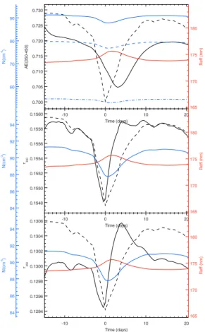
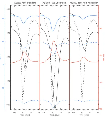
In Fig. 2 the upper plot is the output from a single run with κ=1.5 days,

PH₂SO₄=20 000 cm−

3

s−1,s=0.001 cm−3s−1and shows the Angstrom exponent (black

line) as a function of the 36 days representing the FD (black dashed). The effective

20

radius (red) as well as the number of H2SO4particles: Ntotal(blue solid),N>3 nm (blue

dashed) andN>100 nm (blue point-dashed) is also shown. The two lower plots gives

the optical depths atλ=350 and 450 nm used to calculate the upper plot.

For this choice of parameters it is observed how the Angstrom exponent decreases

by_≈2% to a minimum approximately 3 days after the FD minimum. The explanation

(13)

ACPD

9, 22833–22863, 2009

decreases

T. Bondo et al.

Title Page

Tables Figures

◭ ◮

Back Close

Full Screen / Esc

is that at the onset of the FD the cluster production,s, and hence the number of small

particles decreases. Since the loss rate remains constant this causes the total

par-ticle number to decrease and a subsequent minimum inτ350 is observed around the

time of the FD minimum. A couple of days after the FD minimum the optical depth for

λ=350 nm returns to its initial value. Note that this happens several days before the

5

particle number returns to its original value. The reason being that as the number of particles go down, the remaining ones increase in size, due to reduced competition for the sulphuric acid. As the particle radius increases, so does the optical thickness. The

same pattern is observed forλ=450 nm, however the optical depth increases above its

original value, before it relaxes back. This is due to a higher sensitivity to the particle

10

radius, since this wavelength is further away from the e_ffective radius of the particle

population (174 nm). The difference in behaviour for the optical thickness at the two

wavelengths show the complex dependence of the AOT on particle number and ra-dius. Furthermore this is the reason for the observed lag of 3 days in the dip of the AE compared to the dip in the FD. An obvious interpretation of this lag, if seen in

observa-15

tional data, would be to attribute it to the time it takes from the decrease in production of small particles to propagate up to sizes detectable at the employed wavelengths. Our analysis, however, shows that this is not the only possible explanation, but that the increase in radius of the remaining population must also be considered.

5 Output of model from parameter space

20

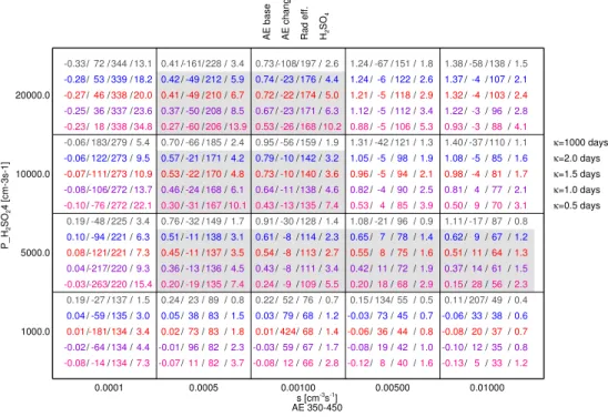
In Fig. 3 the whole parameter space is explored. Each box represents a value ofsand

PH₂SO₄. In each box the colors represent the loss values ofκ=0.5,1,1.5,2,1000 days

increasing from a value of 0.5 days (bottom) to 1000 days (top). For each loss value the first number gives the base level of the Angstrom exponent defined as the mean

of the first 10 days of Angstrom exponent output (t=−15 to−5 in Fig. 3). The second

25

number is then the per mille deviation of the largest extremum of day₋5–20 from the

(14)

ACPD

9, 22833–22863, 2009

decreases

T. Bondo et al.

Title Page

Tables Figures

◭ ◮

Back Close

Full Screen / Esc

following numbers are the mean of the 10 first days of the effective radius in nm and

sulphuric acid concentration in cm−3(divided by 107), respectively.

Three types of responses are behind the different percentage responses. The

stan-dard case is the one outlined in Sect. 4 where a small dip appears in the Angstrom exponent. However, in a few cases the choice of input parameters gives a peak in the

5

Angstrom exponent indicating that a decrease in small particle population may also

lead to increases in AE. This happens when the effective radius gets below a certain

point around 80 nm (depending somewhat onsandPH₂SO₄), far away from the probing

wavelengths of 350 and 450 nm. A switch in sensitivity then seems to happen causing

the low wavelength to be more sensitive to the change in effective radius than the high

10

wavelength, as opposed to what was seen in the single run of Sect. 4. Since the AOT at 350 nm then increases the most as the radius of the particle population grows, this causes an increase in the AE. The third response is the case where no mixing occurs

(κ=1000 days). Here very large changes in the AE is typically observed. These rather

large percentage changes are more a result of an unstable initial precondition run than

15

a real decrease in Angstrom exponent caused by the modulation of cluster production. When there is no loss for the particles, steady state is never reached and therefore

the effective radius continues to grow, causing a decrease of the AE, throughout these

runs. Since the AE is then much lower after the FD, simply because of this overall

growth of the population, artificially high changes appear. The runs withκ=1000 days

20

should generally be regarded with care.

For a constant loss rate and cluster production an increase in PH₂SO₄ in general

leads to higher Angstrom exponent base level. This is explained by the larger increase in available condensable gas enabling better growth of the smaller particles. This will cause the optical depth to increase for 350 nm and hence the Angstrom exponent to

in-25

crease. Note also that the effective radius increases withPH₂SO₄, in all cases. However,

if the effective radius gets too high then an increase inPH₂SO₄can cause a decrease in

AE level since the sensitivity of the AOT at 450 starts to increase. Similarly, for a

(15)

ACPD

9, 22833–22863, 2009

decreases

T. Bondo et al.

Title Page

Tables Figures

◭ ◮

Back Close

Full Screen / Esc

exponent base level. This is natural since higher half lives results in fewer small parti-cles being removed.

And again, for a constant loss rate and sulphuric acid production an increase ins in

general leads to higher Angstrom exponent base level. This is explained by an increase in the number concentration of smaller particle, causing the AOT at 350 nm to increase

5

at a higher rate than at 450 nm. Additionally a highs leads to a decrease in effective

radius, due to an increased competition for the sulphuric acid. In a few cases this

actu-ally causes the AE to decrease assincreases (for instance forPH₂SO₄=1000.0 cm−

3

s−1

ands going from 0.00500 to 0.01000 cm−3s−1.

As can be observed the baseline values vary from small negative numbers to a

10

maximum around 1.4 in Angstrom exponent. In Sano (2004) the average Angstrom exponent over the ocean is about 0.5. In Kazil et al. (2006) and Weber et al. (2001) the sulphuric acid concentration over the oceans was found based on both modelling and measurements. Here values of sulphuric acid concentration in the lower troposphere

over the ocean was about 107cm−3. If these values are compared with our results this

15

can be used to restrict the solution space of sulphuric acid production and cluster

pro-duction to the region 0.0005 cm−3s−1_≤s _≤0.001 cm−3s−1 andP_H

2SO4≥5000 cm

−3

s−1

and the region 0.005 cm−3s−1_≤s_≤0.01 cm−3s−1withPH₂SO₄=5000 cm−

3

s−1. This

re-gion is shaded in grey in the figure and indicates the most probable optical response in the marine troposphere to Forbush decreases under the assumption of a square root

20

dependency of the cluster formation rate to the ion production. As can be observed the expected average change in percentage of the Angstrom exponent is of the order

of−6 to 3% in the shaded region, compared to the initial 10% modulation in ionization.

The AE change is a function of the relative change in the two optical depths. These in turn depend strongly on particle size and number. Ignoring negative AE base levels and

25

those very close to 0 there does seem to be some trends in the AE change. When the

effective radius increase so does the AE change (for constant half-lifes). This is seen

clearly, for instance, forPH₂SO₄going from 5000 cm−

3

s−1to 20 000 cm−3s−1, for all

(16)

ACPD

9, 22833–22863, 2009

decreases

T. Bondo et al.

Title Page

Tables Figures

◭ ◮

Back Close

Full Screen / Esc

switches from negative to positive. An example of this is forPH₂SO₄=5000 cm−

3

s−1and

s going from 0.001 to 0.005 cm−3s−1. These results indicate that wavelengths close to

the effective radius of the particle population are best suited for making observations

of the response in AE to Forbush decreases.

Finally, a similar analysis was performed for the wavelength pair of 550–900 nm. The

5

reason for selecting this wavelength pair is that the MODIS instrument (Platnick et al., 2003) as well as AERONET measures these or similar wavelength pairs. However, this wavelength pair probes sizes of the particle distribution where almost no particles remain. Therefore smaller decreases or increases (of the order of maximum 1%) in the Angstrom exponent are observed. This will be elaborated on in Sect. 8 where the

10

model results are compared with observations.

6 Modifying the sea salt distribution

The sea salt modes used in this study are described in Sect. 2.3. In this section we examine the sensitivity of our results to changes in these modes.

Natural sea salt can have a wide range of sizes (Pierce and Adams, 2006), from a

15

few nano meter (Clarke et al., 2006) and up to micrometers (O’Dowd et al., 1999). Due to limitations in the available data for refractive indices we have limited our sensitivity study to variations in the two modes provided by OPAC. Firstly a run, based on the case in Fig. 2, was made where all sea salt was removed, to gauge the overall contribution of the sea salt to the optical parameters. The AE increased from 0.72 to 1.14 which

20

is well in line with the understanding that smaller particles yield higher AE. The optical thicknesses at 350 nm and 450 nm dropped by 0.045 and 0.046, respectively. The base values were 0.156 and 0.130, meaning that the sea salt contributes 29% to the optical thickness at 350 nm and 36% at 450 nm.

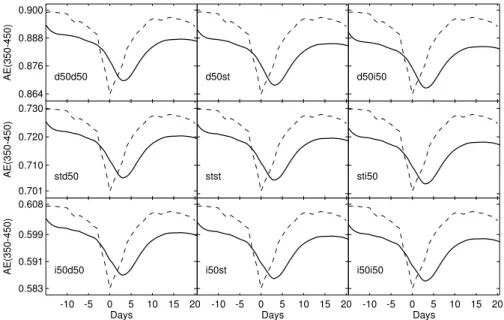
Figure 4 shows the output of 9 different runs, again based on the case in Fig. 2,

25

(17)

ACPD

9, 22833–22863, 2009

decreases

T. Bondo et al.

Title Page

Tables Figures

◭ ◮

Back Close

Full Screen / Esc

have been run with its standard value(st)provided by OPAC, a 50% decrease (d50),

and a 50% increase (i50), producing the 9 plots shown in the figure, such that d50i50 means that the accumulation mode has been decreased by 50% and the coarse mode increased similarly. The strongest response in the AE comes from changes in the ac-cumulation mode, which is to be expected since the median size of this mode (209 nm)

5

is much closer to the wavelengths used to find the AE (350 nm and 450 nm) compared

with the coarse mode (1.75µm). Changing the accumulation mode of sea salt by 50%

in either direction shifts the baseline of the AE by about 20%. Similar changes in the coarse mode only yields very small changes in the AE.

Interestingly the dip in AE due to the Forbush decrease seems to be more or less

10

undisturbed by the changes in sea salt, changing from 2.2% in the d50d50 case to 2.3% for i50i50. For the run with no sea salt the dip is also 2.2%. To investigate this further a run was made where the amount of sea salt was increased to an amount corresponding

to a high wind speed of 18 m2. This was done using the empirical law found by Mulcahy

et al. (2008), stating that the marine aerosol optical thickness scales with the square of

15

the windspeed. The AE thus decreased to 0.28 and the dip increased to 2.7%. These runs show that the amount of sea salt mostly serves as a sort of baseline change to the

optical thickness and thus AE, whereas the dip in the AE is not affected greatly. The

caveat here is that a change in sea salt would normally be accompanied by a change

in loss rate for the nucleated particles, which is not modeled here. Instead e_ffects of

20

changing loss rates are looked at separately in Sect. 5.

7 Modifying cluster formation rate

The responses shown in the previous section are dependent on how ionization influ-ences cluster formation. Based on results from Svensmark et al. (2007) a square root dependency of the cluster formation rate was assumed (see Sect. 3). This however is

25

(18)

ACPD

9, 22833–22863, 2009

decreases

T. Bondo et al.

Title Page

Tables Figures

◭ ◮

Back Close

Full Screen / Esc

sections.

Figure 5 shows the result from the single run (see Sect. 4) with the two alternate nucleation schemes as presented in Sect. 3. The left plot is identical to upper plot in Fig. 2. In the middle plot a linear dependency of the cluster formation rate to the ion-ization is examined. Here it can be seen that removing the square root dependency

5

increases the dip in Angstrom exponent by about 50% due to the larger variations in cluster formation rate. In the right plot the cluster formation is again assumed to have a square root dependency and additionally 50% of the perturbation by the FD is now removed by adding a constant term to the time varying cluster production. Here the

re-sponse goes down with about 50%. This means that the effect of Forbush decreases is

10

dependent on both how ionization affect nucleation as well as the ratio of effectiveness

of the different competing nucleation mechanisms in the marine troposphere.

8 Comparison with observations

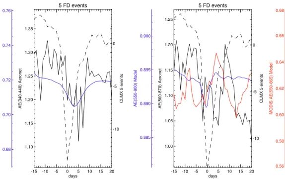
Svensmark et al. (2009) made an epoch analysis of AERONET data from 5 major FD events. Angstrom exponent data (340–440 nm) from approximately 40 stations

15

(stations with more than 20 measurements a day) were superposed and averaged over the 5 events (31 October 2003, 13 September 2005, 19 January 2005, 16 July 2000, 12 April 2001). In this section we compare those results with the model runs. Additionally we investigate the wavelength pair 550, 900 nm which can be compared with both AERONET and MODIS data.

20

The left of Fig. 6 shows a comparison of Angstrom exponents for the short wave-length pair from the model (350, 450 nm) and from the average of the 5 FDs from AERONET (340, 440 nm). The right of Fig. 6 shows the wavelength pairs AERONET (500, 870 nm), MODIS (550, 865 nm), and Model (550, 900 nm). The dashed line is the average of the FD signal over the events listed above. First, it is observed that the

25

(19)

ACPD

9, 22833–22863, 2009

decreases

T. Bondo et al.

Title Page

Tables Figures

◭ ◮

Back Close

Full Screen / Esc

due to aerosols from e.g. pollution, dust, and biomass burnings.1

The left figure shows a slight significant signal for the short wavelength pair for AERONET where a decrease in the Angstrom exponent is observed a couple of days after the FD minimum for the 5 events. However, for the longer wavelength pairs in the right figure both for MODIS and AERONET no significant signal seem to be present.

5

Since we are comparing an ocean based model with land based observations no di-rect comparison can be made but we can however point to some trends. There is a systematic decrease of a factor of approximately 2–4 in signal for going from the small wavelength pair to the larger in our model. Assuming that the weak signal observed in Svensmark et al. (2009) is real then the signal from the long wavelength pairs could

10

be lowered into the climatic noise of the Angstrom exponent observations. If a linear

dependency of the cluster formation rate is assumed this e_ffect would even be more

pronounced (see Sect. 7). This seems to be confirmed by the left of Fig. 6 although more observations would be needed to examine this in more detail. Therefore if an ion induced mechanism is working as in our model, it is expected that observations based

15

on the shorter wavelength pair would be the most favourable for seeing the FD effect.

9 Summary

Under the assumption that ion induced nucleation play a role in the marine tropo-sphere, a simple aerosol growth model in combination with a Mie scattering code and an optical properties program was used to model Angstrom exponents over the

tro-20

pospheric ocean for two wavelength pairs (350, 450 nm and 550, 900 nm) during a Forbush decrease by modulating the nucleation rate over time by the ionization profile from the Forbush decrease. The marine environment was modeled by a fixed-in-time

1

(20)

ACPD

9, 22833–22863, 2009

decreases

T. Bondo et al.

Title Page

Tables Figures

◭ ◮

Back Close

Full Screen / Esc

bimodal sea salt distribution and a variable sulphuric acid aerosol distribution. A large parameter space was explored by altering nucleation mode cluster production rates, sulphuric acid production, loss rates, as well as exploring alternative nucleation mech-anism. Distinct but highly varying responses in the optical properties were found by changing the initial parameter settings. For the short wavelength pair (350, 450 nm)

5

changes in the Angstrom exponent of about−6 to 3% was found for realistic settings

of the Angstrom exponent base level values and sulphuric acid concentration as com-pared to the marine troposphere. For the longer wavelength pair (550, 900 nm) the changes were generally a factor of 2–4 lower. This seems to match with observations from AERONET and MODIS were an epoch analysis of 5 major FD event reveal a slight

10

significant signal in the wavelength pair (340, 440 nm) and not in the longer wavelength pair (550, 900 nm).

The study encourages more global observations of Angstrom exponents at smaller wavelength pairs and improving the signal to noise ratio further. This may help to improve the understanding of the importance of ion induced nucleation and of how

15

secondary aerosol distributions affect the marine optical properties. Future work

re-lated to the model should focus on implementing a dynamic sea salt distribution and investigating other nucleation schemes and growth rates further.

References

Arnold, F.: Multi-ion complexes in the stratosphere – Implications for trace gases and aerosol,

20

Nature, 284, 610–611, 1980. 22836

Cane, H.: Coronal mass ejections and forbush decreases, Space Sci. Rev., 93, 55–77, 2000. 22835

Clarke, A., Owens, S., and Zhou, J.: An ultrafine sea-salt flux from breaking waves: Implications for cloud condensation nuclei in the remote marine atmosphere, J. Geophys. Res.-Atmos.,

25

111, doi:10.1029/2005JD006565, 2006. 22848

(21)

ACPD

9, 22833–22863, 2009

decreases

T. Bondo et al.

Title Page

Tables Figures

◭ ◮

Back Close

Full Screen / Esc

aerosol-formation: First observational evidence from aircraft-based ion mass spectrometer measurements in the upper troposphere, Geophys. Res. Lett., 29, 43–1, 2002. 22836

Enghoff, M. B., Pedersen, J. O. P., Bondo, T., Johnson, M. S., Paling, S., and Svensmark, H.:

Evidence for the Role of Ions in Aerosol Nucleation, J. Phys. Chem. A, 112, 10305–10309, doi:10.1021/jp806852d, 2008. 22836, 22839

5

Forbush, S. E.: On the Effects in Cosmic-Ray Intensity Observed During the Recent Magnetic

Storm, Physical Review, 51, 1108–1109, doi:10.1103/PhysRev.51.1108.3, 1937. 22835

Harrison, R. G. and Stephenson, D. B.: Empirical evidence for a nonlinear effect of galactic

cosmic rays on clouds, Proceedings of the Royal Society A, 462, 1221–1233, 2006. 22835 Hess, M., Koepke, P., and Schult, I.: Optical Properties of Aerosols and Clouds: The Software

10

Package OPAC., B. Am. Meteorol. Soc., 79, 831–844, doi:10.1175/1520-0477(1998)079, 1998. 22837, 22839, 22840

Hirsikko, A., Yli-Juuti, T., Neiminen, T., Vartiainen, E., Laakso, L., Hussein, T., and Kulmala, M.: Indoor and outdoor air ions and aerosol particles in the urban atmosphere of Helsinki: characteristics, sources and formation, Boreal Environ. Res., 12, 295–310, 2007. 22836

15

Holben, B., Eck, T., Slutsker, I., Tanr ´e, D., Buis, J., Setzer, A., Vermote, E., Reagan, J., Kauf-man, Y., Nakajima, T., Lavenu, F., Jankowiak, I. and Smirnov, A.: AERONET – A federated instrument network and data archive for aerosol characterization, Rem. Sens. Environ, 66, 1–16, 1998. 22836, 22841, 22857

Kazil, J., Lovejoy, E. R., Barth, M. C., and O’Brien, K.: Aerosol nucleation over oceans and the

20

role of galactic cosmic rays, Atmos. Chem. Phys., 6, 4905–4924, 2006, http://www.atmos-chem-phys.net/6/4905/2006/. 22841, 22847

Kim, T. O., Adachi, M., Okuyama, K., and Seinfeld, J. H.: Experimental Measurement of

Com-petitive Ion-Induced and Binary Homogeneous Nucelation in SO₂/H₂O/N₂Mixtures, Aerosol

Sci. Tech., 26, 527–543, 1997. 22836

25

Kniveton, D. R.: Precipitation, cloud cover and Forbush decreases in galactic cosmic rays, J. Atmos. Terr. Phys., 66, 1135–1142, 2004. 22835

Kristj ´ansson, J. E., Stjern, C. W., Stordal, F., Fjraa, A. M., Myhre, G., and J ´onasson, K.: Cosmic rays, cloud condensation nuclei and clouds a reassessment using MODIS data, Atmos. Chem. Phys., 8, 7373–7387, 2008,

30

http://www.atmos-chem-phys.net/8/7373/2008/. 22835

(22)

ACPD

9, 22833–22863, 2009

decreases

T. Bondo et al.

Title Page

Tables Figures

◭ ◮

Back Close

Full Screen / Esc

doi:10.1029/2009GL037584, 2009. 22837

Kulmala, M., Riipinen, I., Sipil ä, M., Manninen, H. E., Pet äj ä, T., Junninen, H., Dal Maso, M., Mordas, G., Mirme, A., Vana, M., Hirsikko, A., Laakso, L., Harrison, R. M., Hanson, I., Leung, C., Lehtinen, K. E. J., and Kerminen, V.-M.: Toward Direct Measurement of Atmospheric Nucleation, Science, 318, 89–92, doi:10.1126/science.1144124, 2007. 22836

5

Laakso, L., M ¨akel ¨a, J. M., Pirjola, L., and Kulmala, M.: Model studies on ion-induced nucleation in the atmosphere, J. Geophys. Res. Atmos., 107, 4427–4445, doi:10.1029/2002JD002140, 2002. 22836, 22838, 22839

Laakso, L., Gagn é, S., Pet äj ä, T., Hirsikko, A., Aalto, P. P., Kulmala, M., and Kerminen, V.-M.: Detecting charging state of ultra-fine particles: instrumental development and ambient

10

measurements, Atmospheric Chemistry and Physics, 7, 1333–1345, 2007. 22836

Laaksonen, A., Vesala, T., Kulmala, M., Winkler, P. M., and Wagner, P. E.: Commentary on

cloud modelling and the mass accommodation coe_fficient of water, Atmos. Chem. Phys., 5,

461–464, 2005,

http://www.atmos-chem-phys.net/5/461/2005/. 22838

15

Lee, S.-H., Reeves, J. M., Wilson, J. C., Hunton, D. E., Viggiano, A. A., Miller, T. M., Ballenthin, J. O., and Lait, L. R.: Particle Formation by Ion Nucleation in the Upper Troposphere and Lower Stratosphere, Science, 301, 1886–1889, doi:10.1126/science.1087236, 2003. 22836 Lehtinen, K. E. J. and Kulmala, M.: A model for particle formation and growth in the atmosphere

with molecular resolution in size, Atmos. Chem. Phys. Discuss., 2, 1791–1807, 2002,

20

http://www.atmos-chem-phys-discuss.net/2/1791/2002/. 22838

Lovejoy, E. R., Curtius, J., and Froyd, K. D.: Atmospheric ion-induced nucleation of sulfuric acid and water, J. Geophys. Res. Atmos., 109, 1–11, doi:10.1029/2003JD004460, 2004. 22836, 22844

Marsh, N. and Svensmark, H.: Galactic cosmic ray and El Ni ˜no-Southern Oscillation trends in

25

International Satellite Cloud Climatology Project D2 low-cloud properties, J. Geophys. Res. Atmos., 108, 4195–4205, doi:10.1029/2001JD001264, 2003. 22835

Modgil, M., Kumar, S., Tripathi, S., and Lovejoy, E.: A parameterization of ion-induced nucle-ation of sulphuric acid and water for atmospheric conditions, J. Geophys. Res. Atmos., 110, 19, doi:10.1029/2004JD005475, 2005. 22844

30

(23)

ACPD

9, 22833–22863, 2009

decreases

T. Bondo et al.

Title Page

Tables Figures

◭ ◮

Back Close

Full Screen / Esc

O’Dowd, C., McFiggans, G., Creasey, D. J., Pirjola, L., Hoell, C., Smith, M. H., Allan, B. J., Plane, J. M. C., Heard, D. E., Lee, J. D., Pilling, M. J., and Kulmala, M.: On the photochemical production of new particles in the coastal boundary layer, Geophys. Res. Lett., 26, 1707– 1710, doi:10.1029/1999GL900335, 1999. 22848

Pierce, J. and Adams, P.: Global evaluation of CCN formation by direct emission of

5

sea salt and growth of ultrafine sea salt, J. Geophys. Res. Atmos., 111, D06203, doi:10.1029/2005JD006186, 2006. 22848

Pierce, J. R. and Adams, P. J.: Efficiency of cloud condensation nuclei formation from ultrafine

particles, Atmos. Chem. Phys., 7, 1367–1379, 2007,

http://www.atmos-chem-phys.net/7/1367/2007/. 22837, 22841

10

Pierce, J. R. and Adams, P. J.: Can cosmic rays affect cloud condensation nuclei by altering

new particle formation rates?, online available at: http://dx.doi.org/10.1029/2009GL037946

Geophys. Res. Lett., 36, L09820₊, doi:10.1029/2009GL037946, 2009. 22837

Platnick, S., King, M. D., Ackerman, S. A., Menzel, W. P., Baum, B. A., Riedi, J. C., and Frey, R. A.: The MODIS cloud products: algorithms and examples from terra, IEEE Transactions

15

on Geoscience and Remote Sensing, 41, 459–473, doi:10.1109/TGRS.2002.808301, 2003. 22837, 22841, 22848

Pudovkin, M. I. and Veretenenko, S. V.: Cloudiness decreases associated with Forbush de-creases of galactic cosmic rays., J. Atmos. Terr. Phy., 57, 1349–1355, 1995. 22835

Sano, I.: Optical thickness and Angstrom exponent of aerosols over the land and ocean from

20

space-borne polarimetric data, Adv. Space Res., 34, 833–837, 2004. 22847

Schuster, G. L., Dubovik, O., and Holben, B. N.: Angstrom exponent and bimodal aerosol size distributions, J. Geophys. Res. Atmos., 111, 14 pp., doi:10.1029/2005JD006328, 2006. 22836

Seinfeld, J. and Pandis, S.: Atmospheric Chemsitry and Physics : From Air Pollution to Climate

25

Change, Wiley, 2 edn., 2006. 22838, 22842

Sloan, T. and Wolfendale, A. W.: Testing the proposed causal link between cosmic rays and cloud cover, Environ. Res.Lett., 3, p. 024001, doi:10.1088/1748-9326/3/2/024001, 2008. 22835, 22836

Svensmark, H., Pedersen, J. O. P., Marsh, N. D., Enghoff, M. B., and Uggerhøj, U. I.:

Exper-30

imental evidence for the role of ions in particle nucleation under atmospheric conditions, P. Roy. Soc. A, 463, 385–396, doi:10.1098/rspa.2006.1773, 2007. 22843, 22849

(24)

ACPD

9, 22833–22863, 2009

decreases

T. Bondo et al.

Title Page

Tables Figures

◭ ◮

Back Close

Full Screen / Esc

aerosols and clouds, online available at: http://dx.doi.org/10.1029/2009GL038429 Geophys.

Res. Lett., 36, L15101+, doi:10.1029/2009GL038429, , 2009. 22835, 22836, 22850, 22851

Tinsley, B. A.: The global atmospheric electric circuit and its effects on cloud microphysics,

Rep. Prog. Phys., 71, p. 066801, doi:10.1088/0034-4885/71/6/066801, 2008. 22835

Todd, M. C. and Kniveton, D. R.: Short-term variability in satellite-derived cloud cover and

5

galactic cosmic rays: an update, J. Atmos. Terr. Phys., 66, 1205–1211, 2004. 22835

Usoskin, I. G., Gladysheva, O. G., and Kovaltsov, G. A.: Cosmic ray-induced ionization in the atmosphere: spatial and temporal changes, J. Atmos. Sol.-Terr. Phys., 66, 1791–1796, doi:10.1016/j.jastp.2004.07.037, 2004. 22842

Weber, R. J., Chen, G., Davis, D. D., Mauldin III, R. L., Tanner, D. J., Eisele, F. L., Clarke,

10

A. D., Thornton, D. C., and Bandy, A. R.: Measurements of enhanced H₂SO₄ and 3–4 nm

particles near a frontal cloud during the First Aerosol Characterization Experiment (ACE 1), J. Geophys. Res., 106, 24107–24117, doi:10.1029/2000JD000109, 2001. 22841, 22847 Winkler, P. M., Steiner, G., Vrtala, A., Vehkamaki, H., Noppel, M., Lehtinen, K. E. J.,

Reis-chl, G. P., Wagner, P. E., and Kulmala, M.: Heterogeneous nucleation experiments

bridg-15

ing the scale from molecular ion clusters to nanoparticles, Science, 319, 1374–1377, doi:10.1126/science.1149034, 2008. 22836

Wolf, S.: Mie Scattering by Ensembles of Particles with Very Large Size Parameters, Comput. Phys. Commun., 162, 113–123, 2004. 22837, 22839

Yu, F.: From molecular clusters to nanoparticles: second-generation ion-mediated nucleation

20

(25)

ACPD

9, 22833–22863, 2009

decreases

T. Bondo et al.

Title Page

Tables Figures

◭ ◮

Back Close

Full Screen / Esc

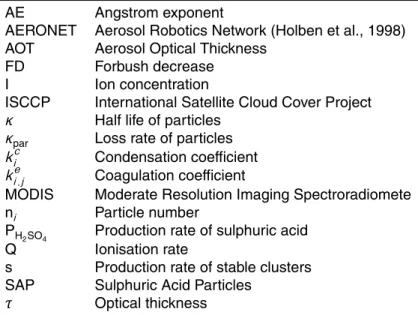
Table 1.List of abbreviations.

AE Angstrom exponent

AERONET Aerosol Robotics Network (Holben et al., 1998)

AOT Aerosol Optical Thickness

FD Forbush decrease

I Ion concentration

ISCCP International Satellite Cloud Cover Project

κ Half life of particles

κ_par Loss rate of particles

k_ic Condensation coefficient

k_{i ,j}e Coagulation coefficient

MODIS Moderate Resolution Imaging Spectroradiomete

n_i Particle number

P_H

2SO4 Production rate of sulphuric acid

Q Ionisation rate

s Production rate of stable clusters

SAP Sulphuric Acid Particles

(26)

ACPD

9, 22833–22863, 2009

decreases

T. Bondo et al.

Title Page

Tables Figures

◭ ◮

Back Close

Full Screen / Esc

Sulphate Aerosol

Growth model

Mie Scattering

Program

Angstrom Exponent Program

OPAC

In

T,N, s(t), P_H2SO4

In

N_ss-accu, N_ss-accu Out

dN(t)_SAP/dlogD_p

Out

WSAPt

Out

Wss-fixed(t)

Results

W_total(t),Dt

In

dN(t)_SAP/dlogD_p,, z,

alt., refr. indices

In

WSAPt,Wss-fixed(t)

(27)

ACPD

9, 22833–22863, 2009

decreases

T. Bondo et al.

Title Page

Tables Figures

◭ ◮

Back Close

Full Screen / Esc

Fig. 2. The upper plot is model output from a single run withκ=1.5 days,p=20000 cm−3s−1, s=0.001 cm−3

s−1and shows the Angstrom exponent (black line) over 36 days for the FD (black

dashed). The effective radius (red) and the number of H₂SO₄ particles: N_total (blue solid),

N>3 nm (blue dashed) and N>100 nm (blue point-dashed) are also shown. The two lower

(28)

ACPD

9, 22833–22863, 2009

decreases

T. Bondo et al.

Title Page Abstract Introduction Conclusions References Tables Figures ◭ ◮ ◭ ◮ Back Close

Full Screen / Esc

Interactive Discussion AE 350-450

0.0001 0.0005 0.00100 0.00500 0.01000 s [cm-3

s-1 ] 1000.0 5000.0 10000.0 20000.0 P_H 2 SO 2 4 [cm-3s-1]

-0.08/ -14/134/ 7.3 -0.02/ -64/134/ 4.4 0.01/-181/134/ 3.4

0.04/ -59/135/ 3.0

0.19/ -27/137/ 1.5

-0.07/ 11/ 82/ 3.7 -0.01/ 96/ 82/ 2.3 0.02/ 73/ 83/ 1.8

0.05/ 38/ 83/ 1.5

0.24/ 23/ 89/ 0.8

-0.08/ 12/ 66/ 2.8 -0.03/ 59/ 67/ 1.7 0.01/ 424/ 68/ 1.4

0.03/ 79/ 68/ 1.2

0.22/ 52/ 76/ 0.7

-0.12/ 8/ 40/ 1.6 -0.08/ 19/ 42/ 1.0 -0.06/ 36/ 44/ 0.8

-0.03/ 73/ 45/ 0.7

0.15/ 134/ 55/ 0.5

-0.13/ 5/ 33/ 1.2 -0.10/ 12/ 35/ 0.8 -0.08/ 20/ 37/ 0.7

-0.06/ 33/ 38/ 0.6

0.11/ 207/ 49/ 0.4

-0.03/-263/220/15.4 0.04/-217/220/ 9.3 0.08/-121/221/ 7.3

0.10/ -94/221/ 6.3

0.19/ -48/225/ 3.4

0.20/ -19/135/ 7.4 0.36/ -13/136/ 4.5 0.45/ -11/137/ 3.5

0.51/ -11/138/ 3.1

0.76/ -32/149/ 1.7

0.24/ -9/109/ 5.5 0.43/ -8/111/ 3.4 0.54/ -8/113/ 2.7

0.61/ -8/114/ 2.3

0.91/ -30/128/ 1.4

0.20/ 18/ 68/ 2.9 0.42/ 11/ 72/ 1.9 0.55/ 8/ 75/ 1.6

0.65/ 7/ 78/ 1.4

1.08/ -21/ 96/ 0.9

0.15/ 28/ 56/ 2.3 0.37/ 14/ 61/ 1.5 0.51/ 11/ 64/ 1.3

0.62/ 9/ 67/ 1.2

1.11/ -17/ 87/ 0.8

-0.10/ -76/272/22.1 -0.08/-106/272/13.7 -0.07/-111/273/10.9

-0.06/ 122/273/ 9.5

-0.06/ 183/279/ 5.4

0.30/ -31/167/10.1 0.46/ -24/168/ 6.1 0.53/ -22/170/ 4.8

0.57/ -21/171/ 4.2

0.70/ -66/185/ 2.4

0.43/ -13/135/ 7.4 0.64/ -11/138/ 4.6 0.73/ -10/140/ 3.6

0.79/ -10/142/ 3.2

0.95/ -56/159/ 1.9

0.53/ 4/ 85/ 3.9 0.82/ -4/ 90/ 2.5 0.96/ -5/ 94/ 2.1

1.05/ -5/ 98/ 1.9

1.31/ -42/121/ 1.3

0.50/ 9/ 70/ 3.1 0.81/ 4/ 77/ 2.1 0.98/ -4/ 81/ 1.7

1.08/ -5/ 85/ 1.6

1.40/ -37/110/ 1.1

-0.23/ 18/338/34.8 -0.25/ 36/337/23.6 -0.27/ 46/338/20.0

-0.28/ 53/339/18.2

-0.33/ 72/344/13.1

0.27/ -60/206/13.9 0.37/ -50/208/ 8.5 0.41/ -49/210/ 6.7

0.42/ -49/212/ 5.9

0.41/-161/228/ 3.4

0.53/ -26/168/10.2 0.67/ -23/171/ 6.3 0.72/ -22/174/ 5.0

0.74/ -23/176/ 4.4

0.73/-108/197/ 2.6

0.88/ -5/106/ 5.3 1.12/ -5/112/ 3.4 1.21/ -5/118/ 2.9

1.24/ -6/122/ 2.6

1.24/ -67/151/ 1.8

0.93/ -3/ 88/ 4.1 1.22/ -3/ 96/ 2.8 1.32/ -4/103/ 2.4

1.37/ -4/107/ 2.1

1.38/ -58/138/ 1.5

AE base AE change Rad eff. H2

SO

4

κ=1000 days

κ=2.0 days

κ=1.5 days

κ=1.0 days

κ=0.5 days

Fig. 3.Model overview of the sensitivity study of various optical parameters and sulphuric acid concentrations as function of loss rates, sulphuric acid production rates and cluster production

rates as described in Sect. 5. Each box represents a value ofsandPH2SO4. In each box the

colors represent the loss values ofκ=0.5,1,1.5,2,1000 days increasing from a value of 0.5

days (bottom) to 1000 days (top). For each loss value the first number gives the base level of the Angstrom exponent defined as the mean of the first 10 days of Angstrom exponent output

(t=−15 to₋5 days). The second number is the per mille deviation of the largest extremum of

days₋5 to 20 from the base level. Positive numbers mean an increase in AE and vice versa.

The two following numbers are the mean of the 10 first days of the effective radius in nm and

sulphuric acid concentration in cm−3

(29)

ACPD

9, 22833–22863, 2009

decreases

T. Bondo et al.

Title Page

Tables Figures

◭ ◮

Back Close

Full Screen / Esc

Interactive Discussion 0.864

0.876 0.888 0.900

AE(350-450) d50d50 d50st d50i50

0.701 0.710 0.720 0.730

AE(350-450) std50 stst sti50

-10 -5 0 5 10 15 20 Days

0.583 0.591 0.599 0.608

AE(350-450) i50d50

-10 -5 0 5 10 15 20 Days

i50st

-10 -5 0 5 10 15 20 Days

i50i50

Fig. 4. Variations of the sea salt distribution. This figure shows the output of 9 runs, based on

the run described in Sect. 4, but with different levels of sea salt. d50 refers to a 50% decrease

in a mode, st to the standard value, and i50 to a 50% increase. The accumulation mode is

(30)

ACPD

9, 22833–22863, 2009

decreases

T. Bondo et al.

Title Page

Tables Figures

◭ ◮

Back Close

Full Screen / Esc

(31)

ACPD

9, 22833–22863, 2009

decreases

T. Bondo et al.

Title Page

Tables Figures

◭ ◮

Back Close

Full Screen / Esc

Interactive Discussion 5 FD events

-15 -10 -5 0 5 10 15 20 days

1.10 1.15 1.20 1.25 1.30 1.35

AE(340-440) Aeronet

0.68 0.70 0.72 0.74 0.76

AE(350-450) Model

-10 -5 0

CLMX 5 events

5 FD events

-15 -10 -5 0 5 10 15 20 days

1.00 1.05 1.10 1.15 1.20 1.25

AE(500-870) Aeronet

0.885 0.890 0.895 0.900

AE(550-900) Model

0.56 0.58 0.60 0.62 0.64 0.66 0.68

MODIS AE(550-865) Model

-10 -5 0

CLMX 5 events