GMDD
8, 3861–3904, 2015CMAQ aerosol size distributions
C. G. Nolte et al.
Title Page
Abstract Introduction
Conclusions References
Tables Figures
◭ ◮
◭ ◮
Back Close
Full Screen / Esc
Printer-friendly Version Interactive Discussion
Discussion
P
a
per
|
Discussion
P
a
per
|
Discussion
P
a
per
|
Discussion
P
a
per
|
Geosci. Model Dev. Discuss., 8, 3861–3904, 2015 www.geosci-model-dev-discuss.net/8/3861/2015/ doi:10.5194/gmdd-8-3861-2015
© Author(s) 2015. CC Attribution 3.0 License.
This discussion paper is/has been under review for the journal Geoscientific Model Development (GMD). Please refer to the corresponding final paper in GMD if available.
Evaluation of the Community Multiscale
Air Quality (CMAQ) model v5.0 against
size-resolved measurements of inorganic
particle composition across sites
in North America
C. G. Nolte1, K. W. Appel1, J. T. Kelly2, P. V. Bhave3, K. M. Fahey1, J. L. Collett Jr.4, L. Zhang5, and J. O. Young1
1
Atmospheric Modeling and Analysis Division, National Exposure Research Laboratory, Office of Research and Development, US Environmental Protection Agency,
Research Triangle Park, North Carolina, USA
2
Air Quality Assessment Division, Office of Air Quality Planning and Standards, US Environmental Protection Agency, Research Triangle Park, North Carolina, USA
3
International Centre for Integrated Mountain Development, Kathmandu, Khumaltar, Lalitpur, Nepal
4
Department of Atmospheric Science, Colorado State University, Fort Collins, Colorado, USA
5
GMDD
8, 3861–3904, 2015CMAQ aerosol size distributions
C. G. Nolte et al.
Title Page
Abstract Introduction
Conclusions References
Tables Figures
◭ ◮
◭ ◮
Back Close
Full Screen / Esc
Printer-friendly Version Interactive Discussion
Discussion
P
a
per
|
Discussion
P
a
per
|
Discussion
P
a
per
|
Discussion
P
a
per
|
Received: 18 April 2015 – Accepted: 29 April 2015 – Published: 19 May 2015 Correspondence to: C. G. Nolte ([email protected])
GMDD
8, 3861–3904, 2015CMAQ aerosol size distributions
C. G. Nolte et al.
Title Page
Abstract Introduction
Conclusions References
Tables Figures
◭ ◮
◭ ◮
Back Close
Full Screen / Esc
Printer-friendly Version Interactive Discussion
Discussion
P
a
per
|
Discussion
P
a
per
|
Discussion
P
a
per
|
Discussion
P
a
per
|
Abstract
This work evaluates particle size-composition distributions simulated by the Commu-nity Multiscale Air Quality (CMAQ) model using Micro-Orifice Uniform Deposit Impactor (MOUDI) measurements at 18 sites across North America. Size-resolved measure-ments of particulate SO24−, NO−3, NH+4, Na+, Cl−, Mg2+, Ca2+ and K+ are compared to 5
CMAQ model output for discrete sampling periods between 2002 and 2005. The ob-servation sites were predominantly in remote areas (e.g. National Parks) in the United States and Canada, and measurements were typically made for a period of roughly one month. For SO24−and NH+4, model performance was consistent across the US and Canadian sites, with the model slightly overestimating the peak particle diameter and 10
underestimating the peak particle concentration compared to the observations. Na+ and Mg2+size distributions were generally well represented at coastal sites, indicating reasonable simulation of emissions from sea spray. CMAQ is able to simulate the dis-placement of Cl−in aged sea spray aerosol, though the extent of Cl−depletion relative to Na+ is often underpredicted. The model performance for NO−3 exhibited much more 15
site-to-site variability than that of SO24−and NH+4, with the model ranging from an under-estimation to overunder-estimation of both the peak diameter and peak particle concentration across the sites. Computing PM2.5from the modeled size distribution parameters rather
than by summing the masses in the Aitken and accumulation modes resulted in diff er-ences in daily averages of up to 1 µg m−3
(10 %), while the difference in seasonal and 20
GMDD
8, 3861–3904, 2015CMAQ aerosol size distributions
C. G. Nolte et al.
Title Page
Abstract Introduction
Conclusions References
Tables Figures
◭ ◮
◭ ◮
Back Close
Full Screen / Esc
Printer-friendly Version Interactive Discussion
Discussion
P
a
per
|
Discussion
P
a
per
|
Discussion
P
a
per
|
Discussion
P
a
per
|
1 Introduction
A detailed understanding of the size, chemical composition, and atmospheric concen-tration of particulate matter (PM) is needed to assess its effects on human health, visibility, ecosystems, and climate. Assessments of these various PM effects are typi-cally done with mathematical models, and our confidence in the models is established 5
through rigorous evaluation against ambient measurements. The mass concentration, size distribution, and bulk chemical composition of atmospheric PM are most often measured separately, and models are typically evaluated against these independent measures (e.g., Simon et al., 2012). However, it is well established that the PM compo-sition varies considerably with particle size, and these size-resolved chemical charac-10
teristics govern the optical and radiative properties of PM. Because the aerodynamic behavior of PM is also a strong function of particle size, the size distributions of diff er-ent chemical componer-ents also influence the human health and environmer-ental effects of PM by affecting where particles deposit in the respiratory tract (Asgharian et al., 2001) or whether they are transported to sensitive ecosystems (Scheffe et al., 2014). 15
Inertial cascade impactors are the most robust devices for collecting size-resolved ambient particles and analyzing their chemical composition (e.g., Marple et al., 1991). Because operating a cascade impactor is labor-intensive and costly, their use has been restricted historically to field studies at individual locations or multi-site cam-paigns within small geographic regions (e.g., Herner et al., 2005). Previously, size-20
composition distributions simulated by the Community Multiscale Air Quality (CMAQ) model were evaluated against Micro-Orifice Uniform Deposit Impactor (MOUDI) mea-surements of inorganic particle components at three coastal urban sites in Tampa, Florida during May 2002 using CMAQ’s standard modal aerosol formulation (Kelly et al., 2010) and a sectional formulation (Nolte et al., 2008). Kelly et al. (2011) evalu-25
GMDD
8, 3861–3904, 2015CMAQ aerosol size distributions
C. G. Nolte et al.
Title Page
Abstract Introduction
Conclusions References
Tables Figures
◭ ◮
◭ ◮
Back Close
Full Screen / Esc
Printer-friendly Version Interactive Discussion
Discussion
P
a
per
|
Discussion
P
a
per
|
Discussion
P
a
per
|
Discussion
P
a
per
|
of total particle volume distributions in Atlanta, and Elleman and Covert (2010) eval-uated predictions of total particle mass in two sub-micron size ranges in the Pacific Northwest. These studies indicate that CMAQ often overpredicts the peak diameter of PM mass-size distributions and the widths of the lognormal particle modes. Kelly et al. (2011) reported that in some urban areas (e.g., Fresno, California) CMAQ adequately 5
predicted the observed peak diameter for inorganic components but overpredicted the peak diameter of the organic and elemental carbon distributions. Overpredictions of particle diameter were found to lead to underpredictions of the PM mass in the sub-2.5 µm size range (PM2.5).
The scarcity of impactor data has prevented any model evaluation of size-10
composition distributions across a continental-scale domain. Such an evaluation would enhance our confidence in models for assessing the human health and ecosystem effects of PM. From 2001–2005, a pair of field campaigns was conducted on a large geographic scale to yield size-segregated impactor measurements of the inorganic PM composition at 14 rural sites across the United States and Canada (Zhang et al., 2008; 15
Lee et al., 2008a). In this paper, we evaluate size-composition distributions modeled by CMAQ against impactor measurements collected during these two campaigns, as well as urban-scale campaigns conducted in Pittsburgh and Tampa. We identify the regions and seasons where model performance is best as well as those where fur-ther model development is needed. Some implications on future evaluations of CMAQ 20
output against routine measurements of PM2.5composition are also discussed.
2 Data
2.1 CMAQ simulations
The measurements used in this study were taken during discrete sampling periods spread across the years 2001–2005; therefore several years of CMAQ model simula-25
GMDD
8, 3861–3904, 2015CMAQ aerosol size distributions
C. G. Nolte et al.
Title Page
Abstract Introduction
Conclusions References
Tables Figures
◭ ◮
◭ ◮
Back Close
Full Screen / Esc
Printer-friendly Version Interactive Discussion
Discussion
P
a
per
|
Discussion
P
a
per
|
Discussion
P
a
per
|
Discussion
P
a
per
|
of CMAQ simulations were conducted, covering the period 2002–2005. The CMAQ model configuration was the same for all simulations, with the only differences being in the year-specific emission and meteorological input data. The simulations utilized CMAQ version 5.0.1, which includes updates to the treatment of anthropogenic fugitive dust and windblown dust (Appel et al., 2013), as well as NH3bi-directional surface
ex-5
change (Bash et al., 2013). The simulations were performed for a domain covering the contiguous United States and southern Canada utilizing 12 km by 12 km horizontal grid spacing and 35 vertical layers, with the top of the lowest model layer at approximately 20 m. Lateral boundary conditions (BCs) for the CMAQ simulations were obtained from monthly median concentrations from a GEOS-Chem (Bey et al., 2001) model simu-10
lation of the year 2005 (the same BCs were used for all four years) using the proce-dure described by Henderson et al. (2014). Other model options employed include the AERO6 aerosol module, the Carbon Bond chemical mechanism that includes toluene and chlorine chemistry (CB05TUCL; Sarwar et al., 2011), and online computation of photolysis rates.
15
Meteorological data were provided from Weather Research and Forecast (WRFv3.3; Skamarock and Klemp, 2008) model version 3.3 simulations of 2002–2005. The WRF model simulations were performed using 35 vertical layers extending up to 50 hPa, the Pleim-Xiu land-surface model (PX-LSM; Pleim and Xiu, 1995), the ACM2 planetary boundary layer (PBL) scheme (Pleim, 2007a, b), the Kain-Fritsch cumulus parame-20
terization scheme (Kain, 2004), the Morrison microphysics scheme (Morrison et al., 2009) and four-dimensional data assimilation with no nudging in the PBL. Version 4.0 of the Meteorology Chemistry Interface Processor (MCIPv4.0; Otte and Pleim, 2010) was used to prepare WRF outputs for CMAQ using the same 35-layer vertical structure as in WRF.
25
GMDD
8, 3861–3904, 2015CMAQ aerosol size distributions
C. G. Nolte et al.
Title Page
Abstract Introduction
Conclusions References
Tables Figures
◭ ◮
◭ ◮
Back Close
Full Screen / Esc
Printer-friendly Version Interactive Discussion
Discussion
P
a
per
|
Discussion
P
a
per
|
Discussion
P
a
per
|
Discussion
P
a
per
|
2002) and the 2005 NEI for 2005. Continuous emission monitoring (CEM) data were used for the electric generating units sector. Wildfire emissions were based on daily fire detections from the Hazard Mapping System and the Sonoma Technology SMART-FIRE system (Raffuse et al., 2009).
Hourly mobile emissions were created using year-specific traffic and meteorologi-5
cal data in version 2010b of the Motor Vehicle Emission Simulator (MOVESv2010b; http://www.epa.gov/otaq/models/moves). PM2.5emissions of eight trace metals, includ-ing Mg2+, Ca2+, and K+, were speciated using the profiles in Reffet al. (2009). Other model configuration options affecting emissions include online emissions of accumula-tion and coarse mode Na+, Cl−, SO2−
4 , Mg
2+, Ca2+, and K+from sea spray (Kelly et al.,
10
2010), online NO emissions using lightning flash counts from the National Lightning Detection Network (NLDN; Allen et al., 2012); BELD3 land-use for gridded fractional crop distributions; version 3.1.4 of the Biogenic Emissions Inventory System (BEIS v3.1.4; Vukovich and Pierce, 2002) for online biogenic emissions; the 2001 version of the National Land Characterization Database (NLCD) for land-use data; and NH3
15
emissions from fertilizer based on an Environmental Policy Integrated Climate (EPIC; Cooter et al., 2012) simulation using 2002 fertilizer sales data.
2.2 MOUDI measurements
The MOUDI measurements used in this study are from four distinct datasets, with one dataset consisting of observations from wilderness sites located in several Canadian 20
provinces (Zhang et al., 2008), another set consisting of sites primarily located in US National Parks (Malm et al., 2005; Lee et al., 2008a), a smaller dataset from sites available during the Bay Region Atmospheric Chemistry (BRACE) study in Tampa, Florida (Evans et al., 2004), and finally a dataset collected during the Pittsburgh Air Quality Study (Cabada et al., 2004). Data are available from 18 distinct sites covering 25
GMDD
8, 3861–3904, 2015CMAQ aerosol size distributions
C. G. Nolte et al.
Title Page
Abstract Introduction
Conclusions References
Tables Figures
◭ ◮
◭ ◮
Back Close
Full Screen / Esc
Printer-friendly Version Interactive Discussion
Discussion
P
a
per
|
Discussion
P
a
per
|
Discussion
P
a
per
|
Discussion
P
a
per
|
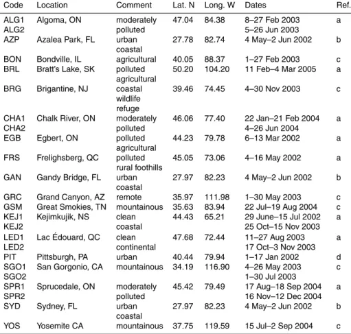
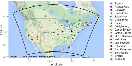
distributions for multiple locations across the US and Canada and under diverse me-teorological conditions. A brief description of the MOUDI data is provided below and a summary of the site locations and observation dates is provided in Table 1, with locations illustrated in Fig. 1.
Aerosol ion (SO24−, NO−3, NH+4, Cl−, Na+, Mg2+, Ca2+and K+) size distributions were 5
measured at eight Canadian sites (i.e. ALG, BRL, CHA, EGB, FRS, KEJ, LED and SPR) (Zhang et al., 2008). The number of samples and the sample duration varied among monitors, with 7 being the fewest and 24 being the most samples taken during any one observation period, while the shortest sample duration was 6 h and the longest 152 h. Standard ion chromatography was used for analyses of all filters after extraction 10
in deionized water. Additional details regarding these measurements can be found in Zhang et al. (2008).
Size distributions of the same particle ions were collected at the BON, SGO, GRC, GSM, YOS and BRG sites in the US. To ensure adequate mass collection at these rural locations, samples were typically collected over a 48 h period, with the exception 15
of Yosemite NP which used 24 h sampling periods. A total of seven study periods are available from these sites in 2002–2004, with one study period in 2002 from mid-July through mid-August (YOS), five study periods in 2003 occurring in February (BON), April (SGO1), May (GRC), July (SGO2) and November (BRG), and one study period in 2004 from mid-July through mid-August (GSM). Additional details regarding these data 20
can be found in Lee et al. (2008a).
Aerosol ion size distributions in three urban locations were collected during the BRACE study in Florida in 2002 at the AZP, GAN and SYD sites and in PIT in Jan-uary 2002 (Table 1). Similar to the other two datasets described above, the BRACE data were collected using MOUDI samplers with 8 or 10 fractionation stages, an inlet 25
height of 2 m, and a flow rate of 30 L min−1for sample durations of approximately 23 h.
GMDD
8, 3861–3904, 2015CMAQ aerosol size distributions
C. G. Nolte et al.
Title Page
Abstract Introduction
Conclusions References
Tables Figures
◭ ◮
◭ ◮
Back Close
Full Screen / Esc
Printer-friendly Version Interactive Discussion
Discussion
P
a
per
|
Discussion
P
a
per
|
Discussion
P
a
per
|
Discussion
P
a
per
|
regarding the BRACE data can be found in Evans et al. (2004) and Nolte et al. (2008), while additional details on the Pittsburgh data can be found in Cabada et al. (2004) and Stanier et al. (2004).
2.3 Data pairing and analysis
The particle size distribution data consist of multiple measurements taken over a period 5
of several weeks. Since the analysis is focused on broad persistent features rather than day-to-day variability, the data here are averaged into a single observed and modeled size distribution for each ion for each campaign listed in Table 1, where the model out-put is averaged over the days and times corresponding to each sampling period. The CMAQ aerosol model uses three lognormal modes (Aitken, accumulation, and coarse) 10
to represent particle size distributions (Binkowski and Roselle, 2003), whereas the ob-servations are separated into discrete size bins. To facilitate comparison between the model and the observations, the three modes in the model are summed to produce a single smooth curve. For each modej, mass concentrationsMj =P
i
Mi j are obtained
from the CMAQ hourly average concentration (ACONC) files, where Mi j is the mass 15
of constituenti in mode j. Modal parameters Dg,j, σg,j, and M3,j are taken from the aerosol diagnostic (AERODIAM) files, whereDg,j is the geometric number mean diam-eter of modej,σg,j is the geometric standard deviation of modej, andM3,j is the third moment of modej. Particle densitiesρj (g cm−3) are calculated as
ρj =10
−12
M3,j 6
πMj. (1)
20
The geometric volume mean diametersDgv are calculated from the number mean di-ameters using the Hatch–Choate relation
Dgv,j =Dg,jp
GMDD
8, 3861–3904, 2015CMAQ aerosol size distributions
C. G. Nolte et al.
Title Page
Abstract Introduction
Conclusions References
Tables Figures
◭ ◮
◭ ◮
Back Close
Full Screen / Esc
Printer-friendly Version Interactive Discussion
Discussion
P
a
per
|
Discussion
P
a
per
|
Discussion
P
a
per
|
Discussion
P
a
per
|
where the multiplication by pρ
j puts the expression in terms of the particle
aerody-namic diameter for consistency with the measurements. The size distribution at each hourtis then computed as
dM
d lnDp(Dp,t)=
3 X
j=1
Mj
√
2πlnσg,j
exp−(lnDp−lnDgv,j)
2
2ln2σg,j (3)
The above equation is discretized by lnDp, and the discretized values are computed 5
for each hour before finally computing the temporally averaged size distribution. For Aitken and accumulation mode species, the inputs to Eq. (3) are obtained di-rectly from CMAQ outputs, but didi-rectly emitted coarse mode species require special processing. In CMAQ v5.0, accumulation mode emissions from sea spray are chem-ically speciated into Na+, Cl−, SO2−
4 , Mg 2+
, Ca2+, and K+ components, but coarse 10
mode sea spray cations are lumped into a single species, ASEACAT, for computational efficiency during advection. Concentrations of individual chemical components in the coarse mode are computed from ASEACAT, soil dust (ASOIL), and coarse primary emissions (ACORS):
ANAK=0.8373·ASEACAT+0.0626·ASOIL+0.0023·ACORS (4)
15
AMGK=0.0997·ASEACAT+0.0032·ACORS (5)
AKK=0.0310·ASEACAT+0.0242·ASOIL+0.0176·ACORS (6)
ACAK=0.0320·ASEACAT+0.0838·ASOIL+0.0562·ACORS (7)
In Equations (4)–(7), ANAK, AMGK, AKK, and ACAK are coarse mode Na+, Mg2+, K+, and Ca2+, respectively, and the coefficients are relative abundances in seawater 20
GMDD
8, 3861–3904, 2015CMAQ aerosol size distributions
C. G. Nolte et al.
Title Page
Abstract Introduction
Conclusions References
Tables Figures
◭ ◮
◭ ◮
Back Close
Full Screen / Esc
Printer-friendly Version Interactive Discussion
Discussion
P
a
per
|
Discussion
P
a
per
|
Discussion
P
a
per
|
Discussion
P
a
per
|
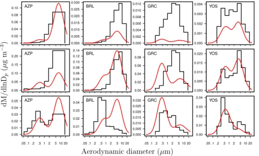
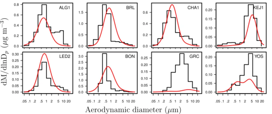
3 Evaluation of size distributions
In this section CMAQ modeled size-composition distributions are compared to the MOUDI measurements. For brevity, a few representative sites and time periods are presented for each ion. Plots of the average modeled and measured size distributions for all 24 campaigns listed in Table 1 are available in the Supplement for each of the 5
inorganic ions analyzed.
3.1 SO2−
4 and NH
+
4
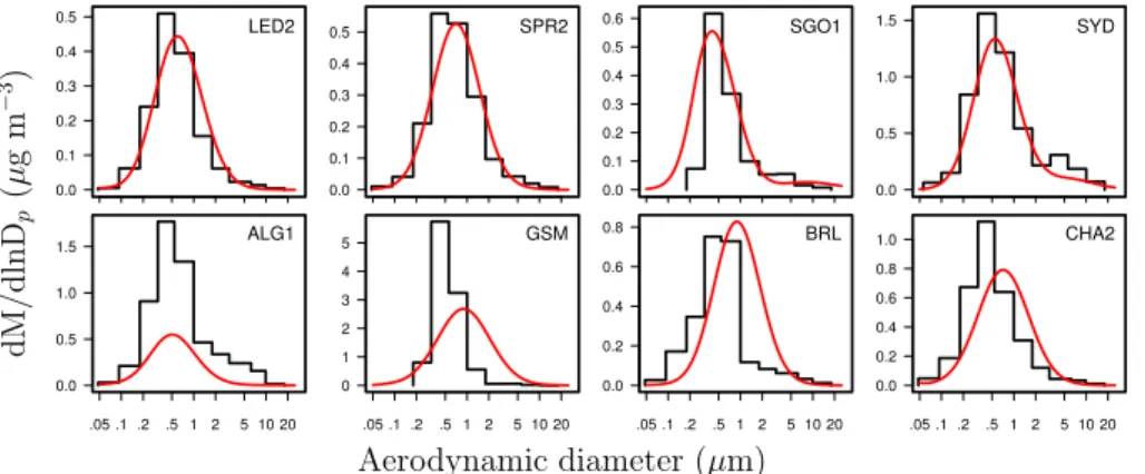
Modeled and observed SO24− size distributions at each site and averaged over each sampling campaign are shown in Supplement Fig. S1. The model generally captures the variability in the SO2−
4 size distribution across different sites and different seasons.
10
As shown in Fig. 2, the model accurately reproduces the observed SO2−
4 size
distribu-tion at many sites, including LED2, SPR2, SGO1, and SYD. However, the model fails to capture the accumulation mode peak observed in many of the campaigns (e.g., ALG1 and GSM), and often the modeled peak diameter is shifted to larger sizes (e.g., BRL and CHA2) than indicated by the measurements.
15
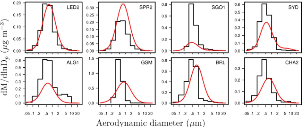
The model performance for particle NH+4 (Fig. 3 and Supplement Fig. S2) generally follows that of SO2−
4 , with the model tending to underestimate the accumulation mode
peak concentration and overestimating the aerodynamic diameter where the peak oc-curs. Modeled and observed NH+4 size distributions are generally in good agreement at those sites where SO24−performance is best (i.e., LED2, SPR2, and SYD), though there 20
is a large NH+4 underprediction at SGO1 in contrast to good SO24− performance there. This behavior is consistent with recent studies that have reported that NH3 emissions
in southern California’s South Coast Air Basin are underestimated in the NEI (Nowak et al., 2012; Kelly et al., 2014). Similarly to the performance for SO24−, the model largely underestimates the NH+4 accumulation mode peak and overestimates the diameter at 25
GMDD
8, 3861–3904, 2015CMAQ aerosol size distributions
C. G. Nolte et al.
Title Page
Abstract Introduction
Conclusions References
Tables Figures
◭ ◮
◭ ◮
Back Close
Full Screen / Esc
Printer-friendly Version Interactive Discussion
Discussion
P
a
per
|
Discussion
P
a
per
|
Discussion
P
a
per
|
Discussion
P
a
per
|
3.2 Na+
and Cl−
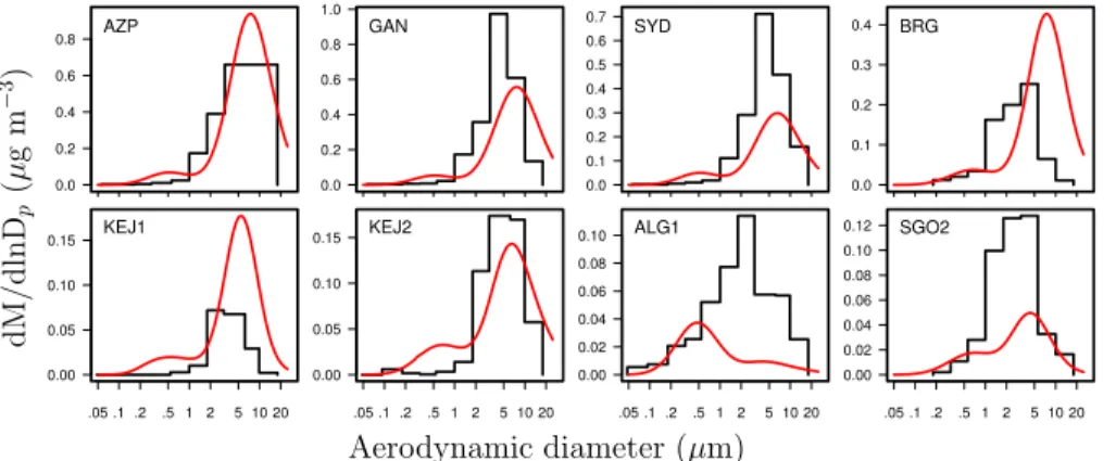
Sea spray is the principal source of Na+ and, at most locations, the dominant source of Cl− as well. Average modeled and observed Na+ size distributions are plotted for the coastal and near-coastal sites in Fig. 4. Cl−size distributions generally follow those
for Na+ and accordingly they are not further discussed here, though Na+and Cl− plots 5
across all the campaigns are presented in Supplement Figs. S3 and S4. CMAQ gen-erally captures the Na+ size distributions and elevated concentrations at the coastal sites, i.e., the BRACE sites (AZP, GAN, and SYD), as well as BRG and KEJ. At most of the other sites, Na+concentrations are very low; often concentrations at these sites are near the detection limit, and confidence in the measurements is relatively low (Zhang 10
et al., 2008). CMAQ correctly simulates that Na+ concentrations are low at these low-concentration sites, though size distributions do not agree very well with measurements (Supplement Fig. S3). The ALG site near Lake Superior is not impacted by sea spray; the relatively high Na+ concentrations in ALG1 are due to the application of salt to roads to prevent ice formation during the winter (Zhang et al., 2008). As this Canadian 15
road salt is not in the US NEI, it is not surprising that the model is unable to capture this peak. SGO is in a mountainous wilderness area about 100 km from the Pacific Ocean. Because simulating winds over mountainous terrain is challenging, particularly with 12 km grid cells, CMAQ’s relatively poor performance for Na+ at SGO2 is likely attributable to errors in transport to the SGO site.
20
The concentration of Cl−in fresh sea spray aerosol is proportional to its abundance in seawater. While Na+ and other sea salt cations are chemically inert, under certain conditions Cl− in aged sea spray particles can be displaced by condensed gas-phase
acids, such as HNO3. The percentage of chloride depleted can be defined as (Yao and
Zhang, 2012) 25
Cl−
depletion(%)=
α[Na+]−[Cl−]
GMDD
8, 3861–3904, 2015CMAQ aerosol size distributions
C. G. Nolte et al.
Title Page
Abstract Introduction
Conclusions References
Tables Figures
◭ ◮
◭ ◮
Back Close
Full Screen / Esc
Printer-friendly Version Interactive Discussion
Discussion
P
a
per
|
Discussion
P
a
per
|
Discussion
P
a
per
|
Discussion
P
a
per
|
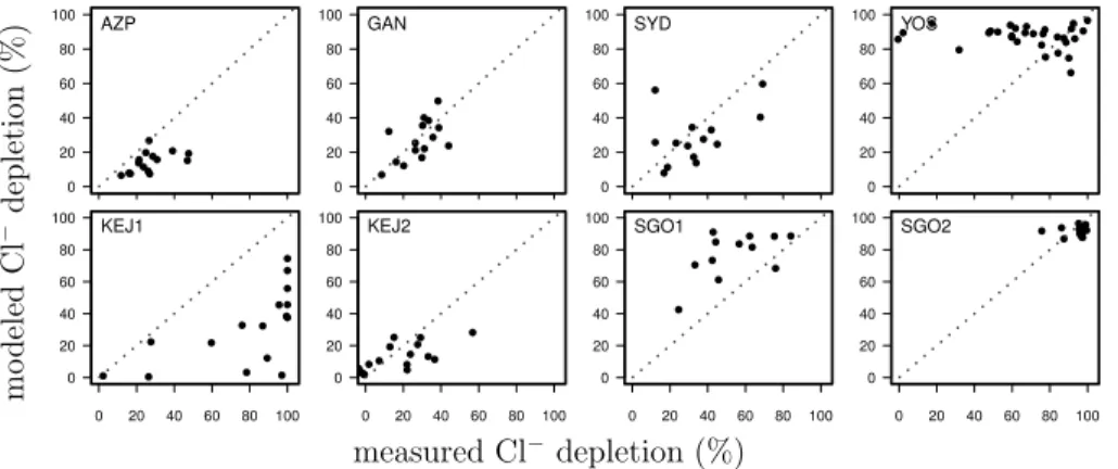
where [Na+] and [Cl−] are molar equivalent concentrations andα is the ratio of the rel-ative molar abundance of Cl− to Na+ in seawater, equal to 1.164 in CMAQ. The mod-eled percentages of chloride depletion are compared to the individual measurements at near-coastal sites in Fig. 5. Consistent with previous results of Kelly et al. (2010), the model frequently underestimates the moderate (25–50 %) levels of chloride depletion 5
seen at the BRACE sites (AZP, GAN, and SYD), which are within 20 km or less from Tampa Bay. The negative bias in the amount of chloride depletion is slightly greater at BRG (not shown). For the rural coastal KEJ site in Nova Scotia, the model slightly underestimates the chloride depletion during the fall campaign (KEJ2), but severely un-derestimates the frequently near-total depletion observed during the summer (KEJ1) 10
(Yao and Zhang, 2012). For the springtime campaign SGO1, the modeled Cl− de-pletion is overestimated. There are significant contributions of sodium from the primary species ASOIL and ACORS for SGO1, which could be contributing to an overprediction of Na+and hence an overprediction of Cl−depletion. For the summer SGO2 campaign, the model correctly simulates chloride depletions approaching 100 %, while at YOS the 15
modeled degree of chloride depletion is sometimes greater than observed. Highly time-resolved measurements were made using a Particle-Into-Liquid Sampler (PILS) at the same locations and times as the MOUDI measurements that are the focus of this study (Lee et al., 2008b). The PILS measurements show that NO−3 peaks coincide with Cl− dropping below detection limits at YOS and SGO2, providing strong evidence of chlo-20
ride displacement from condensation of HNO3. The PILS data further demonstrate that aerosol concentrations varied substantially on much shorter timescales than could be captured by the integrated MOUDI measurements, which partially accounts for the scatter in Fig. 5.
3.3 Mg2+
, Ca2+
and K+
25
GMDD
8, 3861–3904, 2015CMAQ aerosol size distributions
C. G. Nolte et al.
Title Page
Abstract Introduction
Conclusions References
Tables Figures
◭ ◮
◭ ◮
Back Close
Full Screen / Esc
Printer-friendly Version Interactive Discussion
Discussion
P
a
per
|
Discussion
P
a
per
|
Discussion
P
a
per
|
Discussion
P
a
per
|
GAN, SYD, BRG, KEJ1, KEJ2, ALG1, and SGO2 (Supplement Fig. S6), the observed and modeled Mg2+ size distributions have the same relationship to each other as the corresponding Na+ size distributions at those sites. At BRL, GRC, and YOS, Mg2+ is likely to have a crustal rather than oceanic origin. At these western sites, Mg2+is under-predicted (Fig. 6), consistent with findings of Appel et al. (2013). Unlike the behavior for 5
Mg2+, modeled Ca2+is notably underpredicted at coastal sites (Fig. 6 and Supplement Fig. S7). This suggests that there is a source of Ca2+ at those sites not captured by the model. On the other hand, modeled Ca2+ is higher than modeled Mg2+ at BRL, GRC, and YOS, in better agreement with observations, indicating that the coarse mode Ca2+ at those sites is due to contributions from anthropogenic fugitive dust or soils rather 10
than sea spray. The chemical speciation of windblown dust and directly emitted coarse PM is derived from four California desert soil profiles in SPECIATE. Because these profiles did not report Mg, these sources do not contribute to Mg2+ concentrations modeled by CMAQ. The relatively good model performance for Ca2+and underpredic-tion of Mg2+ at these sites suggest that the Mg2+ speciation factors for primary coarse 15
PM and windblown dust should be revisited.
Model performance for K+is notably better than for Ca2+, with the model reasonably capturing the observed pattern at most sites (Fig. 6 and Supplement Fig. S7). K+ is known to be emitted from biomass burning in addition to the sea spray and dust sources that also impact Ca2+. The impact of the combustion source of K+ is evident in the 20
smaller peak diameters for the K+than the Mg2+and Ca2+ observed distributions. The model simulates a bimodal distribution at GRC where the observed distribution was a broad single mode, and the coarse mode is underpredicted at YOS. Overall however, the model does well in simulating the observed K+ particle distribution at the majority of the Canadian and US sites.
25
3.4 NO−
3
Aerosol NO−3 is formed almost entirely from condensation of gas-phase HNO3on
thermo-GMDD
8, 3861–3904, 2015CMAQ aerosol size distributions
C. G. Nolte et al.
Title Page
Abstract Introduction
Conclusions References
Tables Figures
◭ ◮
◭ ◮
Back Close
Full Screen / Esc
Printer-friendly Version Interactive Discussion
Discussion
P
a
per
|
Discussion
P
a
per
|
Discussion
P
a
per
|
Discussion
P
a
per
|
dynamically driven, and is a strong function of inorganic particle composition as well as temperature and relative humidity. As a result, the NO−3 size distribution depends on the distribution of other ions, especially SO24−and NH+4, making it particularly challeng-ing to model accurately (Fig. 7 and Supplement Fig. S8). Model performance for NO−3 is generally good at ALG1, CHA1, and KEJ1, though the coarse mode is somewhat 5
underpredicted at these sites, while the accumulation mode is slightly overpredicted at LED2. Despite the greater surface area of the fine modes, NO−3 often resides in the coarse mode when the fine modes are too acidic from condensation of H2SO4, which has lower vapor pressure than HNO3under ambient conditions. At BRL and BON, the
modeled size distribution is broader and shifted slightly to larger particles than mea-10
sured by the MOUDI. At SGO1 and YOS, particle NO−3 is significantly underestimated. These errors in modeled NO−3 concentrations can be attributed to underestimated lev-els of accumulation-mode NH+4 at SGO1 and underestimated coarse-mode Na+at YOS (cf. Fig. 7 and Supplement Fig. S3).
4 Modeled PM2.5 15
In the US as well as many other countries, air quality regulations for particulate matter are based on the total mass of particles with aerodynamic diameters less than 2.5 µm (PM2.5). Most CMAQ model evaluations, however (e.g., Appel et al., 2008), have used the sum of PM in the Aitken (i) and accumulation (j) modes (i.e. PMi j), to represent
PM2.5. As noted by Jiang et al. (2006), PMi j and PM2.5are conceptually distinct
quan-20
tities that sometimes differ significantly. Since the release of CMAQ v4.5 in 2005, addi-tional variables are output to an opaddi-tional diagnostic file (i.e., AERODIAM) that facilitate a more rigorous calculation of modeled PM2.5based on the simulated size distribution.
GMDD
8, 3861–3904, 2015CMAQ aerosol size distributions
C. G. Nolte et al.
Title Page
Abstract Introduction
Conclusions References
Tables Figures
◭ ◮
◭ ◮
Back Close
Full Screen / Esc
Printer-friendly Version Interactive Discussion
Discussion
P
a
per
|
Discussion
P
a
per
|
Discussion
P
a
per
|
Discussion
P
a
per
|
we compare modeled PM2.5 to the traditional PMi j calculations and to observed total
PM2.5from the IMPROVE, CSN and AQS networks for 2002.
The mass-weighted fractions of the accumulation mode and coarse mode in the PM2.5 size range averaged over the summer and winter seasons are shown in Fig. 8.
Although during the winter the vast majority of the accumulation mode is smaller than 5
2.5 µm, during the summer up to 10–12 % of the accumulation mode is greater than 2.5 µm in size. The smaller fraction of the accumulation mode in the PM2.5 size range
in the eastern US is attributable to larger amounts of aerosol water, both because of higher humidities and higher concentrations of hygroscopic SO24−. The fractional con-tribution of the coarse mode to PM2.5 is fairly uniform, ranging from 10–15 %, though
10
there are a few areas where the contribution exceeds 20 %. Modeled PM2.5 is 0.3– 1.2 µg m−3 lower than PMi j across a large portion of the eastern US during the
sum-mer (Fig. 9), primarily due to the greater contributions of SO24−, NO−3, NH+4 and EC to PMi j than PM2.5 concentrations. In the western US, PM2.5 values are sporadically higher (primarily in Texas, New Mexico, Arizona and southern California) due almost 15
exclusively to the greater contributions of soil (i.e. Al, Si, Ca, Fe and Ti) to PM2.5than
PMi j that result from the tail of the coarse mode overlapping the PM2.5size range. The relative differences are 4–12 % in the eastern US during summer and 4–20 % in the western US (Supplement Fig. S9).
Histograms of the difference in CMAQ daily mean aerosol concentrations (modeled 20
PM2.5 − modeled PMi j) at IMPROVE, CSN and AQS-FRM sites for 2002 are also
shown in Fig. 9. The distribution of mean differences is predominantly negative, par-ticularly during summer and fall (not shown), indicating that PMi j is generally greater than PM2.5. For all seasons, the differences in PM2.5 and PMi j typically fall between
±1 µg m−3.
25
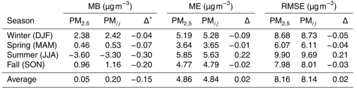
The mean bias (MB), mean error (ME) and root mean square error (RMSE) as com-puted against the IMPROVE, CSN and AQS-FRM observations using modeled PM2.5
GMDD
8, 3861–3904, 2015CMAQ aerosol size distributions
C. G. Nolte et al.
Title Page
Abstract Introduction
Conclusions References
Tables Figures
◭ ◮
◭ ◮
Back Close
Full Screen / Esc
Printer-friendly Version Interactive Discussion
Discussion
P
a
per
|
Discussion
P
a
per
|
Discussion
P
a
per
|
Discussion
P
a
per
|
winter, spring, and fall, average PM2.5 is 0.04–0.20 µg m− 3
less than PMi j. Since the
model is generally positively biased with respect to observations during those sea-sons, using PM2.5rather than PMi j results in slightly improved performance statistics. The difference between PM2.5 and PMi j is larger (more negative) during the summer,
and since the model is generally negatively biased then, the MB, ME, and RMSE are 5
all slightly worse for PM2.5 than for PMi j. The differences during the summer are still small, however, averaging 0.30 µg m−3for MB, 0.22 µg m−3for ME, and 0.21 µg m−3for RMSE. Overall, the aggregated model performance using modeled PM2.5 and PMi j
is nearly the same, with the average difference (PM2.5−PMi j) in MB, ME and RMSE across all seasons of−0.15, 0.02 and 0.02 µg m−3, respectively. Therefore, while the 10
difference between PM2.5and PMi j values for any particular observation site and time may be important, the difference in model performance between the two values is rela-tively small on average. The difference in the two methods for estimating PM2.5is likely
to be even smaller when the models are applied in a relative sense for a regulatory context (Baker and Foley, 2011).
15
In the version of CMAQ (v4.3) used by Jiang et al. (2006), there was very little mass in the coarse mode, and this mode was modeled as being chemically inert. Thus, PMi j was always greater than PM2.5in that version. Because the model was generally positively biased with respect to measurements, using the size distribution to compute PM2.5improved model performance statistics. There have been several updates to the
20
CMAQ aerosol model since the version used by Jiang et al. (2006). For this discussion, the most significant of these are the reduction of overestimated unspeciated PM2.5(i.e.,
PMOTHER; Appel et al., 2008, 2013; Foley et al., 2010), and the treatment of gas-particle nitrate mass transfer to and from coarse mode gas-particles (Kelly et al., 2010). As a result, the consequence of estimating PM2.5concentrations by using the modeled
25
GMDD
8, 3861–3904, 2015CMAQ aerosol size distributions
C. G. Nolte et al.
Title Page
Abstract Introduction
Conclusions References
Tables Figures
◭ ◮
◭ ◮
Back Close
Full Screen / Esc
Printer-friendly Version Interactive Discussion
Discussion
P
a
per
|
Discussion
P
a
per
|
Discussion
P
a
per
|
Discussion
P
a
per
|
5 Model sensitivities
Four additional simulations are conducted to assess the sensitivity of modeled size distributions to changes in the aerosol model. The “BASE” model configuration used for the sensitivity runs contains various updates from CMAQ v5.0.1, but overall results of the BASE simulation used for these sensitivity studies are very similar to those pre-5
sented in Sect. 3. The three sensitivity studies include an adjustment to the apportion-ment of PM emissions between modes and the impleapportion-mentation of a new gravitational settling scheme, two changes that are planned to be included in CMAQ v5.1 (scheduled for release in fall 2015). In addition, a third simulation is performed where the allowable particle mode widths (i.e. geometric standard deviations) in the model are constrained 10
to a relatively narrow range. The details of each sensitivity analysis are described in the following three sub-sections. The sensitivity tests are each performed for May 2002 and compared to data from the three BRACE sites in Tampa during that month.
5.1 PM emissions adjustment
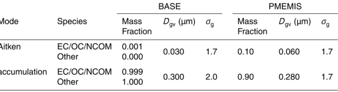
Currently (i.e., in CMAQ v5.0.2), primary anthropogenic emissions of PM2.5
elemen-15
tal carbon (EC), organic carbon (OC), and non-carbonaceous organic matter (NCOM) are mostly (99.9 %) assigned to CMAQ’s accumulation mode, with the remaining 0.1 % assigned to the Aitken mode. Primary anthropogenic emissions of other species (i.e., sulfate, nitrate, chloride, ammonium, sodium, water, and “other”) are 100 % assigned to the accumulation mode. As noted by Elleman and Covert (2010), these modal mass 20
fractions are based on historical measurements that underestimated ultrafine parti-cles. In an effort to improve simulation of aerosol number size distributions, Elleman and Covert (2010) updated particulate emissions size distributions based on a review of modern measurements in regions dominated by urban, power-plant, and marine sources at 4–15 km spatial scales. In the “PMEMIS” sensitivity test, the modal mass 25
emis-GMDD
8, 3861–3904, 2015CMAQ aerosol size distributions
C. G. Nolte et al.
Title Page
Abstract Introduction
Conclusions References
Tables Figures
◭ ◮
◭ ◮
Back Close
Full Screen / Esc
Printer-friendly Version Interactive Discussion
Discussion
P
a
per
|
Discussion
P
a
per
|
Discussion
P
a
per
|
Discussion
P
a
per
|
sions. In addition, the modal parameters characterizing the emitted particles (i.e., ge-ometric mean volume diameter and standard deviation) were modified. The updated emission parameters and their base case values are listed in Table 3. Anthropogenic emissions of coarse PM, as well as sea spray and windblown dust, were unchanged.
The change in particle size distribution for SO24− and Na+ at the three BRACE sites 5
when implementing the PM emissions adjustment is shown in Fig. 10. Particle size distributions are narrower and shifted toward smaller sizes in the PMEMIS simulation compared to the BASE simulation, in better agreement with the observations. This model change affects only the fine mode peak (e.g. SO24−) and does not impact the coarse mode peak (e.g. Na+). Overall, changing the input PM emissions distribution 10
improves CMAQ estimated inorganic particle size distributions compared to the obser-vations.
5.2 Constrained mode widths
CMAQ uses three lognormal modes to model the aerosol size distribution, where each mode is characterized by three parameters: particle number, geometric mean diameter, 15
and geometric standard deviation (Binkowski and Roselle, 2003). Though the mode standard deviations (widths) are calculated as prognostic variables within the aerosol code, they are constrained between the values 1.05 and 2.50. Furthermore, due to numerical instabilities the coarse mode width is not allowed to vary during condensation and evaporation (Kelly et al., 2010). CMAQ mode widths often reach the allowed upper 20
bound, which reduces confidence that they are being simulated accurately. Several other state-of-the-science modal aerosol models use fixed mode widths, e.g., COSMO-ART (Vogel et al., 2009) and MESSy/MADE3 (Kaiser et al., 2014), though other models also allow mode widths to vary (e.g., RAQM2/MADMS; Kajino et al., 2012). To explore how using fixed mode widths might affect CMAQ simulated size distributions, a model 25
GMDD
8, 3861–3904, 2015CMAQ aerosol size distributions
C. G. Nolte et al.
Title Page
Abstract Introduction
Conclusions References
Tables Figures
◭ ◮
◭ ◮
Back Close
Full Screen / Esc
Printer-friendly Version Interactive Discussion
Discussion
P
a
per
|
Discussion
P
a
per
|
Discussion
P
a
per
|
Discussion
P
a
per
|
were constrained between 1.6 and 1.8, while the coarse mode standard deviation was constrained between 2.1 and 2.3.
The difference in particle size distribution between the PMEMIS simulation and the CONSIG simulation is also shown in Fig. 10. Similar to the PMEMIS sensitivity, con-straining the mode widths tends to produce an accumulation mode peak that is nar-5
rower and shifted to smaller sizes than the PMEMIS simulation, resulting in a better comparison against the observations. For the coarse mode however, constraining the mode widths results in a wider and lower peak than the PMEMIS simulations, which does not compare as well to the observations. Of course, the impact on model per-formance is directly dependent on the values chosen to constrain the particle mode 10
widths, and alternative constraints could potentially improve performance for the coarse mode. These results do suggest, however, that the modeled size distribution is sensi-tive to the treatment of the mode widths, and that improvements in the algorithm that computes them would be beneficial.
5.3 Gravitational settling 15
Although the CMAQ aerosol module simulates gravitational settling for particles in the lowest model layer in computing their dry deposition velocities (Binkowski and Roselle, 2003), a potential limitation of the approach is the absence of gravitational settling for particles above layer 1. As a result, coarse particles emitted or convectively mixed above the first model layer can artificially remain aloft and be transported downwind 20
farther than is realistic. As part of the development for CMAQ v5.1, a gravitational settling scheme has been implemented in which settling velocities are calculated for accumulation and coarse mode aerosol zeroth, second, and third moments in each grid cell. The method is a Stokes law approach using the same equations used in computing aerosol deposition velocities to the surface in layer 1 (see Eq. A31–A32 in 25
GMDD
8, 3861–3904, 2015CMAQ aerosol size distributions
C. G. Nolte et al.
Title Page
Abstract Introduction
Conclusions References
Tables Figures
◭ ◮
◭ ◮
Back Close
Full Screen / Esc
Printer-friendly Version Interactive Discussion
Discussion
P
a
per
|
Discussion
P
a
per
|
Discussion
P
a
per
|
Discussion
P
a
per
|
The difference in average Na+ size distributions simulated with and without gravita-tional settling is shown in Fig. 11. Because the impact of gravitagravita-tional settling is signif-icant only for larger particles, there is no discernible effect on the fine-mode range of the aerosol size distribution when gravitational settling is included. However, there is a substantial increase in the coarse-mode size range. The coarse mode peak is higher 5
at the coastal BRACE sites in the GRAV simulation due to particles settling from upper model layers into the lowest model layer, increasing the overall surface layer concen-tration. The impact of gravitational settling is much less significant for inland locations that are not as impacted by sea spray. Including the effects of gravitational settling has only a very minor impact on modeled PM2.5mass.
10
6 Summary and conclusions Size resolved particle ion SO2−
4 , NO−3, NH
+
4, Cl−, Na
+, Mg2+, Ca2+ and K+
measure-ments for sites located throughout the United States and Canada in 2002–2005 were compared to CMAQv5.0.1 model output to assess the ability of the model to repro-duce the observed particle mass size distribution. A total of 24 different measurement 15
campaigns (some sites measured in two different seasons) were available across the four years. The model was generally able to reproduce the observed SO24− and NH+4 distributions at most of the sites, but tended to overestimate the peak diameter and un-derestimate the peak particle concentration. NH+4 was substantially underestimated at the SGO site, likely due to underestimated NH3emissions in California’s South Coast
20
Air Basin.
CMAQ was generally able to capture the size distribution and higher concentrations of Na+and Cl−at coastal and near-coastal sites. The model also reasonably captures Mg2+ concentrations and size distributions for those sites where Mg2+ originates from sea spray (e.g., the three BRACE sites in Florida), but underpredicts at sites influenced 25
GMDD
8, 3861–3904, 2015CMAQ aerosol size distributions
C. G. Nolte et al.
Title Page
Abstract Introduction
Conclusions References
Tables Figures
◭ ◮
◭ ◮
Back Close
Full Screen / Esc
Printer-friendly Version Interactive Discussion
Discussion
P
a
per
|
Discussion
P
a
per
|
Discussion
P
a
per
|
Discussion
P
a
per
|
performance than for Mg2+ at some inland sites, which may be attributable to errors in speciation profiles for various source categories, including windblown and anthro-pogenic fugitive dust. K+, which has contributions from residential wood combustion and wildfires as well as sea spray, exhibits somewhat better model performance than Ca2+. Model performance for NO−3 was mixed, with good performance at some sites 5
(e.g., BRL, CHA1, KEJ1, and LED2), overpredicted concentrations in the accumulation mode size range at some sites (e.g., BRG, FRS, and SPR2), and substantially un-derestimated accumulation mode NO−3 at SGO1 and underestimated coarse particle concentrations at other sites (e.g., GRC, GSM, and YOS).
An examination of the difference in model performance between calculating PM2.5
10
mass from the modeled size distribution or by summing the masses in the Aitken and accumulation modes (PMi j) shows that using the size distribution parameters results in values which on average are smaller by 0.3–1.2 µg m−3. On a daily basis, the difference between PM2.5 and PMi j is usually less than 1 µg m−
3
, regardless of season or year. The largest differences between PM2.5 and PMi j occur in the eastern US during the 15
summer. Concentrations of SO24− are much higher in the eastern US than in the west. Higher humidities in the eastern US, together with the high hygroscopicity of SO24−, lead to growth of the accumulation mode beyond the 2.5 µm size range.
For operational model evaluation, the difference in aggregated model performance between the two methods in comparison to observations is generally very small. Re-20
gional scale assessments based on determination of relative response factors (RRFs), such as development of State Implementation Plans, would likely be unaffected by the choice of using PM2.5 or PMi j. For studies that involve absolute contributions of
PM, particularly at the fine scale, the difference between PM2.5 and PMi j may
war-rant further consideration. The dataset used here, consisting of observations at mostly 25
emis-GMDD
8, 3861–3904, 2015CMAQ aerosol size distributions
C. G. Nolte et al.
Title Page
Abstract Introduction
Conclusions References
Tables Figures
◭ ◮
◭ ◮
Back Close
Full Screen / Esc
Printer-friendly Version Interactive Discussion
Discussion
P
a
per
|
Discussion
P
a
per
|
Discussion
P
a
per
|
Discussion
P
a
per
|
sions, PMi j may be preferable to ensure consistency with emission inventories, as the PM2.5 approach would immediately apportion some fraction of primary emissions to
being outside the 2.5 µm size range. In remote or western regions, however, where PM is highly aged or dust is a main contributor, PM2.5 may be preferable to account for growth outside the 2.5 µm size range or the sub-2.5 µm shoulder of the coarse mode. 5
Two updates to the aerosol model that are scheduled for the next release of CMAQ were evaluated. Increasing the fraction of primary PM emissions apportioned to the Aitken mode from 0.1 to 10 % and modifying the geometric mean diameter and stan-dard deviation of the emitted particles, as recommended by Elleman and Covert (2010), caused the peak diameter of the accumulation mode to decrease, in better agree-10
ment with the observations. Implementing gravitational settling for the accumulation and coarse modes for layers above the lowest model layer led to an increase in coarse mode Na+ from sea spray near the coast. Finally, an experiment in which the mode standard deviations were constrained to a relatively narrow range led to further reduc-tion of accumulareduc-tion mode peak diameters. Given the sensitivity of the size distribureduc-tion 15
to the treatment of mode standard deviations, future work should focus on determining the best approach for representing these variables in the model.
It is important to note that this evaluation of the CMAQ modeled aerosol size distri-butions has focused on the mass size distribution and has considered only inorganic species. As understanding of the health impacts associated with particular PM com-20
ponents and size ranges develops (e.g., Delfino et al., 2011), evaluating predictions of carbonaceous and ultrafine particle size distributions in urban environments could be valuable to support health and exposure applications. Similarly, as the state of the science evolves toward more frequent use of the two-way coupled WRF-CMAQ model (Wong et al., 2012) to capture the influence of air pollution on atmospheric dynamics, 25
GMDD
8, 3861–3904, 2015CMAQ aerosol size distributions
C. G. Nolte et al.
Title Page
Abstract Introduction
Conclusions References
Tables Figures
◭ ◮
◭ ◮
Back Close
Full Screen / Esc
Printer-friendly Version Interactive Discussion
Discussion
P
a
per
|
Discussion
P
a
per
|
Discussion
P
a
per
|
Discussion
P
a
per
|
Code availability
CMAQ model documentation and released versions of the source code are available at www.cmaq-model.org. The updates described here, as well as model postprocessing scripts, are available upon request.
The Supplement related to this article is available online at 5
doi:10.5194/gmdd-8-3861-2015-supplement.
Acknowledgements. We thank Taehyoung Lee (Colorado State University), Noreen Poor (Uni-versity of South Florida), and Charles Stanier (Uni(Uni-versity of Iowa) for providing MOUDI mea-surements that helped make this analysis possible. Brett Gantt and Rohit Mathur (US EPA) provided constructive comments in reviewing this manuscript. We thank Heather Simon and
10
George Pouliot (US EPA) for their assistance with PM profiles in the SPECIATE database. The United States Environmental Protection Agency through its Office of Research and De-velopment supported the research described here. It has been subjected to Agency review and approved for publication. The views and interpretations in this publication are those of the authors and are not necessarily attributable to their organizations.
15
References
Allen, D. J., Pickering, K. E., Pinder, R. W., Henderson, B. H., Appel, K. W., and Prados, A.: Im-pact of lightning-NO on eastern United States photochemistry during the summer of 2006 as determined using the CMAQ model, Atmos. Chem. Phys., 12, 1737–1758, doi:10.5194/acp-12-1737-2012, 2012. 3867
20
GMDD
8, 3861–3904, 2015CMAQ aerosol size distributions
C. G. Nolte et al.
Title Page
Abstract Introduction
Conclusions References
Tables Figures
◭ ◮
◭ ◮
Back Close
Full Screen / Esc
Printer-friendly Version Interactive Discussion
Discussion
P
a
per
|
Discussion
P
a
per
|
Discussion
P
a
per
|
Discussion
P
a
per
|
Appel, K. W., Pouliot, G. A., Simon, H., Sarwar, G., Pye, H. O. T., Napelenok, S. L., Akhtar, F., and Roselle, S. J.: Evaluation of dust and trace metal estimates from the Com-munity Multiscale Air Quality (CMAQ) model version 5.0, Geosci. Model Dev., 6, 883–899, doi:10.5194/gmd-6-883-2013, 2013. 3866, 3874, 3877
Asgharian, B., Hofmann, W., and Bergmann, R.: Particle deposition in a multiple-path model of
5
the human lung, Aerosol Sci. Tech., 34, 332–339, 2001. 3864
Baker, K. R. and Foley, K. M.: A nonlinear regression model estimating single source con-centrations of primary and secondarily formed PM2.5, Atmos. Environ., 45, 3758–3767, doi:10.1016/j.atmosenv.2011.03.074, 2011. 3877
Bash, J. O., Cooter, E. J., Dennis, R. L., Walker, J. T., and Pleim, J. E.: Evaluation of a regional
10
air-quality model with bidirectional NH3exchange coupled to an agroecosystem model, Bio-geosciences, 10, 1635–1645, doi:10.5194/bg-10-1635-2013, 2013. 3866
Bey, I., Jacob, D. J., Yantosca, R. M., Logan, J. A., Field, B. D., Fiore, A. M., Li, Q., Liu, H. Y., Mickley, L. J., and Schulz, M. G.: Global modeling of tropospheric chemistry with assimi-lated meteorology: model description and evaluation, J. Geophys. Res., 106, 23073–23095,
15
doi:10.1029/2001JD000807, 2001. 3866
Binkowski, F. S. and Roselle, S. J.: Models-3 Community Multiscale Air Quality (CMAQ) model aerosol component. 1. Model description, J. Geophys. Res., 108, 4183–4201, 2003. 3869, 3879, 3880
Binkowski, F. S. and Shankar, U.: The Regional Particulate Matter Model 1. Model description
20
and preliminary results, J. Geophys. Res., 100, 26191–26209, 1995. 3880
Cabada, J. C., Rees, S., Takahama, S., Khlystov, A., Pandis, S. N., Davidson, C. I., and Robinson, A. L.: Mass size distributions and size resolved chemical composition of fine particulate matter at the Pittsburgh supersite, Atmos. Environ., 38, 3127–3141, doi:10.1016/j.atmosenv.2004.03.004, 2004. 3867, 3869, 3891
25
Cooter, E. J., Bash, J. O., Benson, V., and Ran, L.: Linking agricultural crop management and air quality models for regional to national-scale nitrogen assessments, Biogeosciences, 9, 4023–4035, doi:10.5194/bg-9-4023-2012, 2012. 3867
Delfino, R. J., Staimer, N., and Vaziri, N. D.: Air pollution and circulating biomarkers of oxidative stress, Air Qual. Atmos. Health, 4, 37–52, doi:10.1007/s11869-010-0095-2, 2011. 3883
30
distri-GMDD
8, 3861–3904, 2015CMAQ aerosol size distributions
C. G. Nolte et al.
Title Page
Abstract Introduction
Conclusions References
Tables Figures
◭ ◮
◭ ◮
Back Close
Full Screen / Esc
Printer-friendly Version Interactive Discussion
Discussion
P
a
per
|
Discussion
P
a
per
|
Discussion
P
a
per
|
Discussion
P
a
per
|
bution of particles emitted into a mesoscale model, J. Geophys. Res., 115, D03204, doi:10.1029/2009JD012401, 2010. 3865, 3878, 3883
Evans, M. C., Campbell, S. W., Bhethanabotla, V., and Poor, N. D.: Effect of sea salt and calcium carbonate interactions with nitric acid on the direct dry deposition of nitrogen to Tampa Bay, Florida, Atmos. Environ., 38, 4847–4858, 2004. 3867, 3869, 3891
5
Foley, K. M., Roselle, S. J., Appel, K. W., Bhave, P. V., Pleim, J. E., Otte, T. L., Mathur, R., Sar-war, G., Young, J. O., Gilliam, R. C., Nolte, C. G., Kelly, J. T., Gilliland, A. B., and Bash, J. O.: Incremental testing of the Community Multiscale Air Quality (CMAQ) modeling system ver-sion 4.7, Geosci. Model Dev., 3, 205–226, doi:10.5194/gmd-3-205-2010, 2010. 3875, 3877 Henderson, B. H., Akhtar, F., Pye, H. O. T., Napelenok, S. L., and Hutzell, W. T.: A database
10
and tool for boundary conditions for regional air quality modeling: description and evaluation, Geosci. Model Dev., 7, 339–360, doi:10.5194/gmd-7-339-2014, 2014. 3866
Herner, J. D., Aw, J., Gao, O., Chang, D. P., and Kleeman, M. J.: Size and com-position distribution of airborne particulate mattern in northern California: I – Par-ticulate mass, carbon, and water-soluble ions, J. Air Waste Manage., 55, 30–51,
15
doi:10.1080/10473289.2005.10464600, 2005. 3864
Houyoux, M. R., Vukovich, J. M., Coats Jr., C. J., Wheeler, N. J. M., and Kasibhatla, P. S.: Emission inventory development and processing for the Seasonal Model for Regional Air Quality (SMRAQ) project, J. Geophys. Res., 105, 9079–9090, 2000. 3866
Jiang, W., Smyth, S., Giroux, É., Roth, H., and Yin, D.: Differences between CMAQ fine mode
20
particle and PM2.5 concentrations and their impact on model performance evaluation in the lower Fraser Valley, Atmos. Environ., 40, 4973–4985, doi:10.1016/j.atmosenv.2005.10.069, 2006. 3875, 3877
Kain, J. S.: The Kain–Fritsch convective parameterization: an update, J. Appl. Meteorol., 43, 170–181, doi:10.1175/1520-0450(2004)043<0170:TKCPAU>2.0.CO;2, 2004. 3866
25
Kaiser, J. C., Hendricks, J., Righi, M., Riemer, N., Zaveri, R. A., Metzger, S., and Aquila, V.: The MESSy aerosol submodel MADE3 (v2.0b): description and a box model test, Geosci. Model Dev., 7, 1137–1157, doi:10.5194/gmd-7-1137-2014, 2014. 3879
Kajino, M., Inomata, Y., Sato, K., Ueda, H., Han, Z., An, J., Katata, G., Deushi, M., Maki, T., Oshima, N., Kurokawa, J., Ohara, T., Takami, A., and Hatakeyama, S.: Development of
30
GMDD
8, 3861–3904, 2015CMAQ aerosol size distributions
C. G. Nolte et al.
Title Page
Abstract Introduction
Conclusions References
Tables Figures
◭ ◮
◭ ◮
Back Close
Full Screen / Esc
Printer-friendly Version Interactive Discussion
Discussion
P
a
per
|
Discussion
P
a
per
|
Discussion
P
a
per
|
Discussion
P
a
per
|
Kelly, J. T., Bhave, P. V., Nolte, C. G., Shankar, U., and Foley, K. M.: Simulating emission and chemical evolution of coarse sea-salt particles in the Community Multiscale Air Qual-ity (CMAQ) model, Geosci. Model Dev., 3, 257–273, doi:10.5194/gmd-3-257-2010, 2010. 3864, 3867, 3873, 3877, 3879
Kelly, J. T., Avise, J., Cai, C., and Kaduwela, A. P.: Simulating particle size distributions
5
over California and impact on lung deposition fraction, Aerosol Sci. Tech., 45, 148–162, doi:10.1080/02786826.2010.528078, 2011. 3864, 3865
Kelly, J. T., Baker, K. R., Nowak, J. B., Murphy, J. G., Markovic, M. Z., VandenBoer, T. C., Ellis, R. A., Neuman, J. A., Weber, R. J., Roberts, J. M., Veres, P. R., de Gouw, J. A., Beaver, M. R., Newman, S., and Misenis, C.: Fine-scale simulation of ammonium and nitrate
10
over the South Coast Air Basin and San Joaquin Valley of California during CalNex-2010, J. Geophys. Res., 119, 3600–3614, doi:10.1002/2013JD021290, 2014. 3871
Lee, T., Yu, X.-Y., Ayres, B., Kreidenweis, S. M., Malm, W. C., and Collett Jr., J. L.: Observations of fine and coarse particle nitrate at several rural locations in the United States, Atmos. Environ., 42, 2720–2732, doi:10.1016/j.atmosenv.2007.05.016, 2008a. 3865, 3867, 3868,
15
3891
Lee, T., Yu, X.-Y., Kreidenweis, S. M., Malm, W. C., and Collett Jr., J. L.: Semi-continuous mea-surement of PM2.5ionic composition at several rural locations in the United States, Atmos. Environ., 42, 6655–6669, doi:10.1016/j.atmosenv.2008.04.023, 2008b. 3873
Malm, W. C., Day, D. E., Carrico, C., Kreidenweis, S. M., Collett Jr., J. L., McMeeking, G.,
20
Lee, T., Carillo, J., and Schichtel, B.: Intercomparison and closure calculations using mea-surements of aerosol species and optical properties during the Yosemite Aerosol Character-ization Study, J. Geophys. Res., 110, D14302, doi:10.1029/2004JD005494, 2005. 3867 Marple, V. A., Rubow, K. L., and Behm, S. M.: A Microorifice Uniform Deposit
Im-pactor (MOUDI): description, calibration, and use, Aerosol Sci. Tech., 14, 434–446,
25
doi:10.1080/02786829108959504, 1991. 3864
Morrison, H., Thompson, G., and Tatarskii, V.: Impact of cloud microphysics on the develop-ment of trailing stratiform precipitation in a simulated squall line: comparison of one- and two-moment schemes, Mon. Weather Rev., 137, 991–1007, doi:10.1175/2008MWR2556.1, 2009. 3866
30
GMDD
8, 3861–3904, 2015CMAQ aerosol size distributions
C. G. Nolte et al.
Title Page
Abstract Introduction
Conclusions References
Tables Figures
◭ ◮
◭ ◮
Back Close
Full Screen / Esc
Printer-friendly Version Interactive Discussion
Discussion
P
a
per
|
Discussion
P
a
per
|
Discussion
P
a
per
|
Discussion
P
a
per
|
a coastal urban site, Atmos. Environ., 42, 3179–3191, doi:10.1016/j.atmosenv.2007.12.059, 2008. 3864, 3869
Nowak, J. B., Neuman, J. A., Bahreini, R., Middlebrook, A. M., Holloway, J. S., McKeen, S. A., Parrish, D. D., Ryerson, T. B., and Trainer, M.: Ammonia sources in the California South Coast Air Basin and their impact on ammonium nitrate formation, Geophys. Res. Lett., 39,
5
L07804, doi:10.1029/2012GL051197, 2012. 3871
Otte, T. L. and Pleim, J. E.: The Meteorology-Chemistry Interface Processor (MCIP) for the CMAQ modeling system: updates through MCIPv3.4.1, Geosci. Model Dev., 3, 243–256, doi:10.5194/gmd-3-243-2010, 2010. 3866
Pleim, J. E.: A combined local and non-local closure model for the atmospheric
bound-10
ary layer. Part 1: Model description and testing, J. Appl. Meteorol. Clim., 46, 1383–1395, doi:10.1175/JAM2539.1, 2007a. 3866
Pleim, J. E.: A combined local and non-local closure model for the atmospheric boundary layer. Part 2: Application and evaluation in a mesoscale model, J. Appl. Meteorol. Clim., 46, 1396– 1409, doi:10.1175/JAM2534.1, 2007b. 3866
15
Pleim, J. E. and Xiu, A.: Development and testing of a surface flux and planetary boundary model for application in mesoscale models, J. Appl. Meteorol., 34, 16–32, doi:10.1175/1520-0450-34.1.16, 1995. 3866
Raffuse, S. M., Pryden, D. A., Sullivan, D. C., Larkin, N. K., Strand, T., and Solomon, R.: SMARTFIRE algorithm description, Sonoma Technol., Inc., Petaluma, Calif., available
20
at: http://firesmoke.ca/smartfire/pdfs/SMARTFIRE_Algorithm_Description_Final.pdf (last ac-cess: 12 May 2015), 2009. 3867
Reff, A., Bhave, P. V., Simon, H., Pace, T. G., Pouliot, G. A., Mobley, J. D., and Houyoux, M.: Emissions inventory of PM2.5trace elements across the United States, Environ. Sci. Technol., 43, 5790–5796, doi:10.1021/es802930x, 2009. 3867
25
Sarwar, G., Appel, K. W., Carlton, A. G., Mathur, R., Schere, K., Zhang, R., and Majeed, M. A.: Impact of a new condensed toluene mechanism on air quality model predictions in the US, Geosci. Model Dev., 4, 183–193, doi:10.5194/gmd-4-183-2011, 2011. 3866
Scheffe, R. D., Lynch, J. A., Reff, A., Kelly, J. T., Hubbell, B., Greaver, T. L., and Smith, J. T.: The Aquatic Acidification Index: a new regulatory metric linking atmospheric and
biogeochemi-30