www.atmos-chem-phys.net/12/2533/2012/ doi:10.5194/acp-12-2533-2012
© Author(s) 2012. CC Attribution 3.0 License.
Chemistry
and Physics
Comment on
“Tropospheric temperature response to stratospheric ozone
recovery in the 21st century” by Hu et al. (2011)
C. McLandress1, J. Perlwitz2, and T. G. Shepherd1
1Department of Physics, University of Toronto, Toronto, Ontario, Canada
2Cooperative Institute for Research in Environmental Sciences University of Colorado/NOAA Earth System Research
Laboratory, Physical Sciences Division, Boulder, CO, USA
Correspondence to:C. McLandress (charles@atmosp.physics.utoronto.ca)
Received: 1 November 2011 – Published in Atmos. Chem. Phys. Discuss.: 14 December 2011 Revised: 15 February 2012 – Accepted: 23 February 2012 – Published: 7 March 2012
Abstract. In a recent paper Hu et al. (2011) suggest that the recovery of stratospheric ozone during the first half of this century will significantly enhance free tropospheric and surface warming caused by the anthropogenic increase of greenhouse gases, with the effects being most pronounced in Northern Hemisphere middle and high latitudes. These sur-prising results are based on a multi-model analysis of CMIP3 model simulations with and without prescribed stratospheric ozone recovery. Hu et al. suggest that in order to properly quantify the tropospheric and surface temperature response to stratospheric ozone recovery, it is necessary to run coupled atmosphere-ocean climate models with stratospheric ozone chemistry. The results of such an experiment are presented here, using a state-of-the-art chemistry-climate model cou-pled to a three-dimensional ocean model. In contrast to Hu et al., we find a much smaller Northern Hemisphere tropo-spheric temperature response to ozone recovery, which is of opposite sign. We suggest that their result is an artifact of the incomplete removal of the large effect of greenhouse gas warming between the two different sets of models.
1 Introduction
Stratospheric ozone depletion has had a radiative effect on global mean surface climate, although the sign of the effect is uncertain due to the large compensation between the short-wave warming due to increased penetration of solar radia-tion and the long-wave cooling due to reduced downwelling infrared radiation from the colder stratosphere (Intergovern-mental Panel on Climate Change (IPCC), 2007; Chapter 10
of SPARC CCMVal, 2010). But all recent estimates (IPCC, 2007; SPARC CCMVal, 2010) are considerably smaller in magnitude than 0.1 W m−2, and thus represent a small num-ber compared to the total radiative forcing. On the other hand, the Antarctic ozone hole, which is a huge perturbation to the Southern Hemisphere (SH) stratosphere, has been the dominant driver of past changes in high-latitude SH tropo-spheric climate in summer (e.g. Arblaster and Meehl, 2006; Fogt et al., 2009), with ozone recovery expected to offset the effects of climate change over the next half-century (e.g. Son et al., 2010). While similar physics might be expected to be at work at high latitudes in the Northern Hemisphere (NH), no such effect has so far been detected there, partly because of the smaller magnitude of ozone depletion in the Arctic, and partly because of the larger impact of greenhouse warm-ing due to meltwarm-ing sea ice (see discussion in Chapter 4 of WMO, 2011).
2534 C. McLandress et al.: Comment on Hu et al. (2011)
mean change of ∼0.41 K over 50 yr (∼0.08 K decade−1).
They also find relatively large enhanced warming in the ex-tratropical and polar regions in summer and autumn in both hemispheres, as well as a significant warming at the surface with a global and annual mean change of∼0.16 K over 50 yr (∼0.03 K decade−1). In fact, the largest warming is found in the NH, which is very surprising given that the changes in stratospheric ozone are much larger in the SH. Further-more the NH high-latitude surface warming maximizes in late fall/early winter, which is also very surprising since the ozone increase maximizes in spring. H11 compare their GCM results to results from a radiative-convective model, and find that although the latter predicts increased warming as ozone levels recover, the tropospheric warming is weaker by a factor of four than that determined from the ensembles of GCMs. They attribute this warming difference to the sim-plicity of their radiative-convective model.
Another possible explanation for the apparently large im-pact of stratospheric ozone recovery on NH temperatures is that their multi-model approach is flawed. Attributing dif-ferences between the two sets of simulations to the effects of ozone recovery is questionable if the signal one is look-ing for is small. Since greenhouse warmlook-ing is expected to dominate the effects of ozone recovery in the NH, small dif-ferences in the tropospheric temperature trends between the two sets of models may simply be a reflection of differences in the GHG-induced warming, and have nothing to do with ozone recovery. Although H11 claim that the mean transient climate response (TCR) of the two sets of models is the same (1.7 K), we compute a difference of 0.22 K for the models used for the future changes, based on the incomplete infor-mation provided in Table 8.2 of IPCC (2007), with the mod-els with ozone recovery having the larger mean TCR. It is therefore plausible that a relatively small difference in the mean TCRs could account for the different rates of tropo-spheric warming in their two sets of model simulations. Fur-thermore, there were differences in the radiative forcings ap-plied to the two sets of models, notably with respect to tropo-spheric ozone where there is a close correspondence between whether or not models included stratospheric ozone recovery and tropospheric ozone changes. Since the projected increase of tropospheric ozone provides a significant GHG warming, especially in the NH, this could also contribute to the NH warming found by H11. Finally, the rate of Arctic warming, which is not encapsulated in a global metric like the TCR, differs from model to model because of different rates of Arc-tic sea ice loss. In fact, Crook and Forster (2011) show that GCMs with large Arctic amplification factors do not neces-sarily have large TCRs. Thus, even if the mean TCRs of the two sets of models were identical, the mean Arctic amplifi-cation factors will almost certainly differ. The enhanced sur-face warming in Arctic winter found by H11 for the models with imposed ozone recovery may therefore be a reflection of that.
In their Conclusion, H11 acknowledge the limitations in their approach and suggest that coupled atmosphere-ocean models including stratospheric ozone chemistry are needed to properly investigate the tropospheric and surface temper-ature responses to stratospheric ozone recovery, in order to avoid this “small difference of large terms” problem. Here, we describe results from such an exercise, using simulations from the Canadian Middle Atmosphere Model (CMAM). By comparing an ensemble of simulations with increasing GHG concentrations and time-varying ozone-depleting substances (ODSs) to an ensemble of simulations with only increasing GHG concentrations (i.e., ODS concentrations held fixed), using the same coupled model, we are able to assess the impact of ozone recovery on tropospheric temperatures in a self-consistent manner. Contrary to the results of H11, we find only a small NH tropospheric temperature response to ozone recovery, which is in fact opposite in sign to theirs.
The outline of our paper is as follows. In Sect. 2 we de-scribe CMAM and the simulations we use. In Sect. 3 we discuss our results. For easy comparison we present many of our results in a similar format to that used by H11. In Sect. 4 we discuss in greater depth the potential causes for the disagreement between our results and those of H11.
2 Description of model and simulations
CMAM is the upward extension of the Canadian Centre for Climate Modelling and Analysis (CCCma) third generation coupled GCM (CGCM3). The ocean component of CMAM is described in McLandress et al. (2010). The atmospheric component has 71 vertical levels, with a resolution that varies from several tens of meters in the lower troposphere to∼2.5 km in the mesosphere. A T31 spectral resolution is used in the horizontal, which corresponds to a grid spacing of∼6◦. Detailed descriptions of the stratospheric chemistry scheme and the atmospheric component of CMAM are provided in de Grandpr´e et al. (2000) and Scinocca et al. (2008), respec-tively.
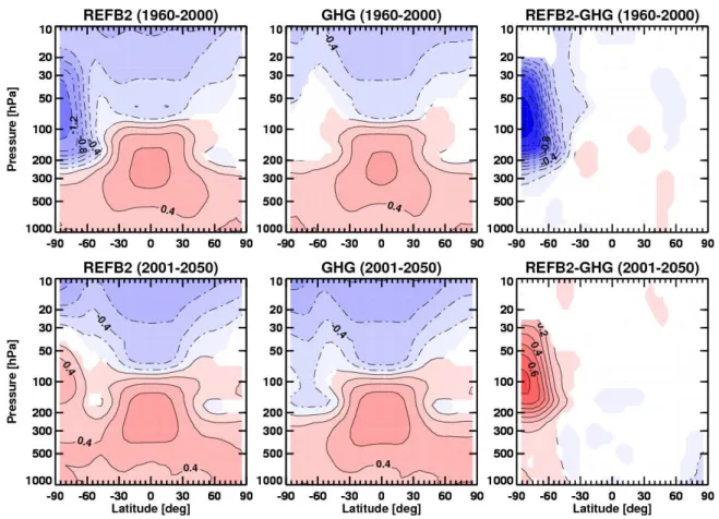
Fig. 1.Annual and zonal mean temperature trends for 1960–2000 (top) and 2001–2050 (bottom): REF-B2 (left), GHG (middle), and REF-B2 minus GHG (right). Contour intervals are 0.2 and 0.1 K decade−1in the two left columns and right columns, respectively, with red denoting positive values and blue negative. Only trends that are significant at the 95 % level are shown.
GHG simulations, as in Plummer et al. (2010). The simula-tions extend from 1960 to 2099, with each set of simulasimula-tions comprising an ensemble of three. Details of the spin-up pro-cedure are given in McLandress et al. (2010).
We present results both for the 1960–2000 (“ozone deple-tion” or “past”) period and the 2001–2050 (“ozone recovery” or “future”) period. Since the sign of the trends driven by changes in stratospheric ozone is expected to change from past to present (e.g., McLandress et al., 2010, 2011), com-paring these two periods helps in assessing the robustness of the results. Linear trends are computed from ensemble mean time series, and their statistical significance is com-puted using the standard t-test (i.e., assuming independent and Gaussian-distributed residuals). All figures show ensem-ble averages.
3 Results
3.1 Annual mean
2536 C. McLandress et al.: Comment on Hu et al. (2011)
Fig. 2.Annual mean temperature trends for 1960–2000 (top) and 2001-2050 (bottom): global average (left), Southern Hemisphere (middle) and Northern Hemisphere (right) for REF-B2 (black), GHG (blue) and REF-B2 minus GHG (red). Error bars denote the 95 % confidence levels of the trends. The insets in the two right panels show blow-ups of the REF-B2-minus-GHG trends in the troposphere.
A more compact way of presenting the annual mean tem-perature trends is by plotting latitudinal averages, as is done in Fig. 2. Shown here are global averages (left), SH average (middle) and NH average (right) for REF-B2 (black), GHG (blue) and REF-B2 minus GHG (red) for the past and future. The two left and bottom right panels are directly comparable to Figs. 2 and 4 of H11. The maximum impact of the ozone changes occurs at∼70 hPa, with the effect being much larger in the SH than in the NH, as expected. We also note that the magnitude of the trends in REF-B2 minus GHG is larger for the past than for the future because the ozone recovery pro-cess is not completed by 2050 (Plummer et al., 2010).
Closer inspection of the right panels of Fig. 2 reveals that below about 300 hPa the 95 % confidence error bars on the red curve do not cross the zero line (see insets), indicating that there is a statistically significant impact of both ozone depletion and ozone recovery on NH average tropospheric temperature. Interestingly, our model results suggest that NH ozone depletion has led to a small tropospheric warm-ing, which would be consistent with ozone depletion exert-ing a net positive radiative forcexert-ing (Chapter 10 of SPARC CCMVal, 2010). Our simulations also suggest that ozone
re-covery will lead to a small tropospheric cooling. However, the magnitude of both the past and future NH tropospheric temperature trends are small (∼0.02 K decade−1 in the up-per troposphere, i.e., about a factor of four smaller than the future warming found by H11).
3.2 Seasonal variation
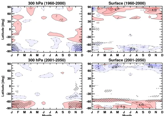
Fig. 3. Zonal mean temperature trend versus month and latitude for REF-B2 minus GHG for 1960–2000 (top) and 2001–2050 (bottom) at 300 hPa (left) and at the surface (right). Contour interval is 0.1 K decade−1, with red denoting positive values and blue negative. Trend magnitudes less than 0.05 K decade−1are not plotted. Cross hatching denotes regions where the 95 % significance level is exceeded.
H11 is absent in our results. Although there are patches of past warming and future cooling in the NH, which are con-sistent with the NH average results shown in Fig. 2, they are not statistically significant when considered regionally and seasonally.
H11 also found large enhanced surface warming in the Arctic during the period of ozone recovery, and suggested that the increasing ozone concentrations are somehow am-plifying the high-latitude response to global warming. The right panels of Fig. 3 show the zonal mean temperature trends at the surface. A comparison of the bottom right panel to Fig. 11 of H11 reveals major differences. H11 reported strong warming in the Arctic, especially in fall and win-ter, while CMAM shows cooling at these latitudes. The Arctic (average over 60–90◦N) surface temperature differ-ence trends averaged from September to January – the time period H11 found to exhibit the maximum warming – ex-hibit a weak but statistically significant cooling in the future (−0.136±0.130 K decade−1).
4 Conclusions
A self-consistent analysis of the possible impact of strato-spheric ozone recovery on tropostrato-spheric temperatures has been undertaken using a version of the Canadian Middle
At-mosphere Model (CMAM) that is coupled to an ocean model. Two sets of simulations are performed: one with time-varying concentrations of GHGs and ODSs, the other with time-varying GHGs and constant ODSs. Although our sim-ulations show the expected large differences in stratospheric temperature changes, we find only a small impact on tropo-spheric temperatures, consistent with the small estimated ra-diative forcing of stratospheric ozone changes (IPCC, 2007; SPARC CCMVal, 2010). Interestingly, the effect in the NH is such that ozone depletion leads to a tropospheric warm-ing, and ozone recovery to a tropospheric coolwarm-ing, which is consistent with ozone depletion representing a positive radia-tive forcing as has been suggested in recent studies (SPARC CCMVal, 2010). It could also represent a climate feedback.
Our results are in striking contrast to those of Hu et al. (2011), who suggest that ozone recovery will have a sub-stantial warming effect in the troposphere (a global and an-nual mean change of∼0.41 K over 50 yr (∼0.08 K decade−1)
2538 C. McLandress et al.: Comment on Hu et al. (2011)
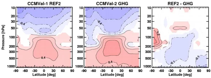
Fig. 4.Annual and zonal mean temperature trends for 2001–2050: CCMVal-1 REF2 (left), CCMVal-2 GHG (middle), and CCMVal-1 REF2 minus CCMVal-2 GHG (right). Contour intervals are 0.2 and 0.1 K decade−1in the two left panels and the right panel, respectively, with red denoting positive values and blue negative. Only trends that are significant at the 95 % level are shown.
(e.g., Son et al., 2010) and sensitivity studies using single models (McLandress et al., 2011; Polvani et al., 2011). The reason why this approach works in the summertime SH is be-cause the Antarctic ozone hole is such a large perturbation to the SH circulation. However, using such an approach in the NH, in particular the Arctic, as H11 do, is problematic since the stratospheric ozone changes in northern high latitudes are considerably weaker, and the GHG-induced warming (which needs to be removed in order to isolate the effects of ozone recovery) is larger.
We suggest that the enhanced tropospheric warming found by H11 results from the comparison of groups of models hav-ing different rates of GHG-induced warmhav-ing; specifically, that differencing the two groups of models does not remove the effect of GHG-induced warming as is needed in order to isolate the effects of ozone recovery. Important regions where such sensitivity to GHG changes becomes obvious are the upper tropical troposphere and the Arctic surface. The rate of upper tropical tropospheric warming is closely related to the rate of surface warming (Arblaster et al., 2011), which is closely linked to the climate sensitivity of the model. For the Arctic, surface warming is strongly determined by the rate of Arctic sea ice loss. Stroeve et al. (2007) showed that CMIP3 models exhibit a large range of declining sea ice ex-tent trends for the period 1953–2006. Thus, compositing two model sets with different sea ice loss rates will result in large apparent effects in Arctic surface temperatures. The season-ality of the Arctic warming determined by H11, with maxi-mum surface warming during late fall/early winter, is consis-tent with the seasonality expected from the impact of Arctic sea ice loss (Deser et al., 2010). This seasonality is not con-sistent with the effect of stratospheric ozone changes, which maximize in spring.
We provide here a simple yet illustrative example of why the method of H11 is inappropriate in the tropical and NH troposphere where the impact of ozone forcing is expected to be small relative to that of other processes. We do this by computing differences in two ensembles of simulations pro-duced using two different versions of CMAM. The first is the “REF2” simulation generated using the CCMVal-1 ver-sion of CMAM (Eyring et al., 2007). Like REF-B2, the REF2 ensemble of three simulations uses time-varying con-centrations of GHGs and ODSs, but unlike REF-B2 it em-ploys prescribed sea-surface temperatures and sea-ice dis-tributions generated using an earlier version of the CCCma coupled atmosphere-ocean model on which that version of CMAM was based. The second set is the GHG simulation using the CCMVal-2 version of CMAM, which has been dis-cussed above. Differencing the two ensemble means is thus analogous to H11 differencing the means of the two different sets of AR4 models with and without ozone recovery.
and 0.20 K decade−1, respectively. Thus, differencing the
two sets of simulations yields the cooling trends seen in the right panel of Fig. 4. The fact that H11 find enhanced warm-ing, while Fig. 4 shows coolwarm-ing, is immaterial since the mean rate of GHG-induced global warming in the CMIP3 models with ozone recovery may simply be larger than in those with-out.
A recent study by Prevedi and Polvani (2012) confirms our hypothesis. They examined the near surface temperature trends in CMIP3 model experiments in which CO2increased
by 1 % per year until doubling. When differencing the same two groups of models as H11, they found remarkably similar results to H11. Since the stratospheric ozone forcing in their two sets of models was identical, the temperature differences could only have arisen from the different responses to the GHG forcing.
In addition, Table 10.1 in IPCC (2007) shows that in most cases, the CMIP3 simulations that include stratospheric ozone recovery also include tropospheric ozone changes, and vice versa. Since the projected increase of tropospheric ozone provides a significant GHG warming, especially in the NH, this could also contribute to the differences found by H11. There were also differences in the groups of models considered by H11 in their treatment of other radiative forc-ing agents such as black carbon, indirect aerosol effect, etc., which further complicates the attribution of enhanced tropo-spheric warming in a specific CMIP3 model group to a single forcing factor like stratospheric ozone recovery.
Although our results are for only a single model (and so are subject to the potential weaknesses of that model), they clearly illustrate the pitfalls in analysing CMIP3 models with and without ozone recovery when trying to quantify the im-pacts of ozone recovery on tropospheric temperatures in the NH. A more definitive analysis would require a multi-model approach using coupled chemistry-climate models or IPCC-like models in which each model performs simulations with and without ozone recovery, and where the ocean and sea ice models coupled to the atmospheric model can respond.
Acknowledgements. The authors thank the three anonymous reviewers for their helpful comments. The CMAM simulations analysed here were produced by the C-SPARC project with funding from the Canadian Foundation for Climate and Atmospheric Sciences. Computing support and funding for CM was provided by Environment Canada. JP acknowledges support from the NASA Modeling and Analysis Program.
Edited by: M. Dameris
References
Arblaster, J. M. and Meehl, G. A.: Contributions of external forc-ings to southern annular mode trends, J. Climate, 19, 2896–2904, 2006.
Arblaster, J. M., Meehl, G. A., and Karoly, D. J.: Future cli-mate change in the Southern Hemisphere: Competing effects of ozone and greenhouse gases, Geophys. Res. Lett., 38, L02701, doi:10.1029/2010GL045384, 2011.
Crook, J. A. and Forster, P. M.: A balance between radia-tive forcing and climate feedback in the modeled 20th cen-tury temperature response, J. Geophys. Res., 116, D17108, doi:10.1029/2011JD015924, 2011.
Deser, C., Tomas, R., Alexander, M., and Lawrence, D.: The seasonal atmospheric response to projected Arctic sea ice loss in the late 21st century, J. Climate, 23, 333–351, 10.1175/2009JCLI3053.1, 2010.
Eyring, V., Waugh, D. W., Bodeker, G. E., Cordero, E., Akiyoshi, H., Austin, J., Beagley, S. R., Boville, B., Braesicke, P., Bruhl, C., Butchart, N., Chipperfield, M. P., Dameris, M., Deckert, R., Deushi, M., Frith, S. M., Garcia, R. R., Gettelman, A., Gior-getta, M., Kinnison, D. E., Mancini, E., Manzini, E., Marsh, D. R., Matthes, S., Nagashima, T., Newman, P. A., Nielsen, J. E., Pawson, S., Pitari, G., Plummer, D. A., Rozanov, E., Schraner, M., Scinocca, J. F., Semeniuk, K., Shibata, K., Steil, B., Sto-larski, R., Tian, W., and Yoshiki, M.: Multimodel projections of stratospheric ozone in the 21st century, J. Geophys. Res., 112, D16303, doi:10.1029/2006JD008332, 2007.
Fogt, R. L., Perlwitz, J., Monaghan, A. J., Bromwich, D. H., Jones, J. M., and Marshall, G. J.: Historical SAM Variability. Part II: Twentieth-Century Variability and Trends from Reconstructions, Observations, and the IPCC AR4 Models, J. Climate, 22, 5346– 5365, 2009.
de Grandpr´e, J., Beagley, S. R., Fomichev, V. I., Griffioen, E., Mc-Connell, J. C., Medvedev, A. S., and Shepherd, T. G.: Ozone cli-matology using interactive chemistry: Results from the Canadian middle atmosphere model, J. Geophys. Res., 105, 26475–26491, 2000.
Hu, Y., Xia, Y., and Fu, Q.: Tropospheric temperature response to stratospheric ozone recovery in the 21st century, Atmos. Chem. Phys., 11, 7687–7699, doi:10.5194/acp-11-7687-2011, 2011. Intergovernmental Panel on Climate Change (IPCC): Climate
Change 2001: The Scientific Basis: Contribution of Working Group I to the Third Assessment Report of the Intergovernmental Panel on Climate Change, edited by: Houghton, J. T., Ding, Y., Griggs, D. J., Noguer, M., van der Linden, P. J., Dai, X. Maskell, K., and Johnson, C. A., Cambridge University Press, New York, USA, 881 pp., 2001.
Intergovernmental Panel on Climate Change (IPCC): Climate Change 2007: The Physical Scientific Basis: Contribution of Working Group I to the Fourth Assessment Report of the Inter-governmental Panel on Climate Change, edited by: Solomon, S., Qin, D., Manning, M., Chen, Z., Marquis, M., Averyt, K. B., Tignor, M., and Miller, H. L., Cambridge University Press, New York, USA, 996 pp., 2007.
2540 C. McLandress et al.: Comment on Hu et al. (2011)
Sigmond, M., Jonsson, A. I., and Reader, M. C.: Separating the dynamical effects of climate change and ozone depletion: Part 2. Southern Hemisphere Troposphere, J. Climate, 23, 5002–5020, doi:10.1175/2010JCLI3586.1, 2011.
Perlwitz, J., Pawson, S., Fogt, R. L., Nielsen, J. E., and Neff, W. D.: Impact of stratospheric ozone hole recovery on Antarctic climate, Geophys. Res. Lett., 35, L08714, doi:10.1029/2008GL033317, 2008.
Plummer, D. A., Scinocca, J. F., Shepherd, T. G., Reader, M. C., and Jonsson, A. I.: Quantifying the contributions to stratospheric ozone changes from ozone depleting substances and greenhouse gases, Atmos. Chem. Phys., 10, 8803–8820, doi:10.5194/acp-10-8803-2010, 2010.
Polvani, L. M., Previdi, M., and Deser, C.: Large cancellation, due to ozone recovery, of future Southern Hemisphere atmo-spheric circulation trends, Geophys. Res. Lett., 38, L04707, doi:10.1029/2011GL046712, 2011.
Previdi, M. and Polvani, L. M.: Comment on “Tropospheric tem-perature response to stratospheric ozone recovery in the 21st cen-tury” by Hu et al. (2011), Atmos. Chem. Phys. Discuss., 12, 2853–2861, doi:10.5194/acpd-12-2853-2012, 2012.
Scinocca, J. F., McFarlane, N. A., Lazare, M., Li, J., and Plummer, D.: Technical Note: The CCCma third generation AGCM and its extension into the middle atmosphere, Atmos. Chem. Phys., 8, 7055–7074, doi:10.5194/acp-8-7055-2008, 2008.
Son, S.-W., Tandon, N. F., Polvani, L. M., and Waugh D. W.: Ozone hole and Southern Hemisphere climate change, Geophys. Res. Lett., 36, L15705, doi:10.1029/2009GL038671, 2009.
Son, S.-W., Gerber, E. P., Perlwitz, J., Polvani, L. M., Gillett, N. P., Seo, K.-H., Eyring, V., Shepherd, T. G., Waugh, D., Akiyoshi, H., Austin, J., Baumgaertner, A., Bekki, S., Braesicke, P., Bruhl, C., Butchart, N., Chipperfield, M. P., Cugnet, D., Dameris, M., Dhomse, S., Frith, S., Garny, H., Garcia, R., Hardiman, S, C., Jockel, P., Lamarque, J. F., Mancini, E., Marchand, M., Mi-chou, M., Nakamura, T., Morgenstern, O., Pitari, G., Plum-mer, D. A., Pyle, J., Rozanov, E., Scinocca, J. F., Shibata, K., Smale, D., Teyssedre, H., Tian, W., and Yamashita, Y.: Im-pact of stratospheric ozone on Southern Hemisphere circula-tion change: A multimodel assessment, J. Geophys. Res., 115, D00M07, doi:10.1029/2010JD014271, 2010.
SPARC CCMVal Report on the Evaluation of Chemistry-Climate Models, edited by: Erying, V., Shepherd, T. G., and Waugh, D. W., SPARC Report No. 5, WCRP-132, WMO/TD-No. 1526, http://www.atmosp.physics.utoronto.ca/SPARC, 2010.
Stroeve, J., Holland, M., Meier, W., Scambos, T., and Serreze, M.: Arctic sea ice decline: Faster than forecast, Geophys. Res. Lett., 34, L09501, doi:10.1029/2007GL029703, 2007.
WMO (World Meteorological Organization)/United Nations Envi-ronment Programme (UNEP), 2006: Scientific assessment of ozone depletion, Global Ozone Res. Monit. Proj. Rep., 50, WMO, Geneva, Switzerland, 2007.