Stratospheric ozone change and related climate impacts over 1850–2100 as modelled by the ACCMIP ensemble

(1)

ACPD

15, 25175–25229, 2015

Stratospheric ozone change and related climate impacts over

1850–2100

F. Iglesias-Suarez et al.

Title Page

Abstract Introduction

Conclusions References

Tables Figures

◭ ◮

Back Close

Full Screen / Esc

Printer-friendly Version

Interactive Discussion

Discussion

P

a

per

|

Discussion

P

a

per

|

Discussion

P

a

per

|

Discussion

P

a

per

|

Atmos. Chem. Phys. Discuss., 15, 25175–25229, 2015 www.atmos-chem-phys-discuss.net/15/25175/2015/ doi:10.5194/acpd-15-25175-2015

This discussion paper is/has been under review for the journal Atmospheric Chemistry and Physics (ACP). Please refer to the corresponding final paper in ACP if available.

Stratospheric ozone change and related

climate impacts over 1850–2100 as

modelled by the ACCMIP ensemble

F. Iglesias-Suarez, P. J. Young, and O. Wild

Lancaster Environment Centre, Lancaster University, Lancaster, UK

Received: 3 July 2015 – Accepted: 20 August 2015 – Published: 15 September 2015

Correspondence to: F. Iglesias-Suarez (n.iglesiassuarez@lancaster.ac.uk)

(2)

ACPD

15, 25175–25229, 2015

1850–2100

Title Page

Tables Figures

◭ ◮

Back Close

Full Screen / Esc

Discussion

P

a

per

|

Discussion

P

a

per

|

Discussion

P

a

per

|

Discussion

P

a

per

Abstract

Stratospheric ozone and associated climate impacts in the Atmospheric Chemistry and Climate Model Intercomparison Project (ACCMIP) simulations are evaluated in the recent past (1980–2000), and examined in the long-term (1850–2100) using the Rep-resentative Concentration Pathways low and high emission scenarios (RCP2.6 and

5

RCP8.5, respectively) for the period 2000–2100. ACCMIP multi-model mean total col-umn ozone (TCO) trends compare favourably, within uncertainty estimates, against observations. Particularly good agreement is seen in the Antarctic austral spring

(−11.9 % dec−1 compared to observed ∼ −13.8±11 % dec−1), although larger

devi-ations are found in the Arctic’s boreal spring (−2.1 % dec−1 compared to observed

10

∼ −5.3±3 % dec−1). The simulated ozone hole has cooled the lower stratosphere

dur-ing austral sprdur-ing in the last few decades (−2.2 K dec−1). This cooling results in

South-ern Hemisphere summertime tropospheric circulation changes captured by an increase

in the Southern Annular Mode (SAM) index (1.27 hPa dec−1). In the future, the interplay

between the ozone hole recovery and greenhouse gases (GHGs) concentrations may

15

result in the SAM index returning to pre-ozone hole levels or even with a more

posi-tive phase from around the second half of the century (−0.4 and 0.3 hPa dec−1for the

RCP2.6 and RCP8.5, respectively). By 2100, stratospheric ozone sensitivity to GHG concentrations is greatest in the Arctic and Northern Hemisphere midlatitudes (37.7

and 16.1 DU diﬀ_{erence between the RCP2.6 and RCP8.5, respectively), and smallest}

20

over the tropics and Antarctica continent (2.5 and 8.1 DU respectively). Future TCO changes in the tropics are mainly determined by the upper stratospheric ozone sensi-tivity to GHG concentrations, due to a large compensation between tropospheric and lower stratospheric column ozone changes in the two RCP scenarios. These results demonstrate how changes in stratospheric ozone are tightly linked to climate and show

25

(3)

ACPD

15, 25175–25229, 2015

1850–2100

Title Page

Tables Figures

◭ ◮

Back Close

Full Screen / Esc

Discussion

P

a

per

|

Discussion

P

a

per

|

Discussion

P

a

per

|

Discussion

P

a

per

|

1 Introduction

The Atmospheric Chemistry and Climate Model Intercomparison Project (ACCMIP) (Lamarque et al., 2013b) was designed to evaluate the long-term (1850–2100) atmo-spheric composition changes (e.g. ozone) to inform the Fifth Assessment Report of the Intergovernmental Panel on Climate Change (IPCC, 2013), supplementing phase

5

5 of the Coupled Model Intercomparison Project (CMIP5) (Taylor et al., 2012), where the focus was more on physical climate change. In addition, ACCMIP is the first model intercomparison project in which the majority of the models included chemi-cal schemes appropriate for stratospheric and tropospheric chemistry. Due to the ab-sorption of shortwave radiation, stratospheric ozone is important for determining the

10

stratospheric climate (e.g. Randel and Wu, 1999) and has a strong influence on tropo-spheric ozone through stratosphere-to-troposphere transport (e.g. Collins et al., 2003; Sudo et al., 2003; Zeng and Pyle, 2003; Hegglin and Shepherd, 2009). In addition,

changes in stratospheric ozone can aﬀ_{ect atmospheric circulation and climate,}

reach-ing to the lower troposphere in the case of the Antarctic ozone hole (e.g. Thompson

15

and Solomon, 2002; Gillett and Thompson, 2003). This study evaluates stratospheric ozone changes and associated climate impacts in the ACCMIP simulations, quantifying the evolution since the pre-industrial period through to the end of the 21st century.

Stratospheric ozone represents approximately 90 % of ozone in the atmosphere and absorbs much of the ultraviolet solar radiation harmful for the biosphere (e.g. WMO,

20

2014; UNEP, 2015). Anthropogenic emissions of ozone depleting substances (ODS) such as chlorofluorocarbons and other halogenated compounds containing chlorine and bromine have played a key role in depleting stratospheric ozone during the latter half of the 20th century (e.g. WMO, 2014). Although present globally averaged TCO

levels are only∼3.5 % lower than pre-1980 values, about half the TCO is depleted over

25

(4)

ACPD

15, 25175–25229, 2015

1850–2100

Title Page

Tables Figures

◭ ◮

Back Close

Full Screen / Esc

Discussion

P

a

per

|

Discussion

P

a

per

|

Discussion

P

a

per

|

Discussion

P

a

per

(e.g. WMO, 2007, 2014). As a result, stratospheric ozone is expected to recover and return to pre-industrial values during the 21st century (Austin and Wilson, 2006; Eyring et al., 2007, 2010a, 2013; Austin et al., 2010). Although anthropogenic ODS are the main cause of ozone depletion over the last decades, other species such as methane,

nitrous dioxide (N2O) and carbon dioxide (CO2) aﬀect stratospheric ozone chemistry

5

as well (Haigh and Pyle, 1982; Portmann et al., 2012; Revell et al., 2012; Reader et al., 2013; Dietmüller et al., 2014). Randeniya et al. (2002) argued that increasing concentrations of methane can amplify ozone production in the lower stratosphere via photochemical production, though increases of water vapour from methane oxidation

may have the opposite eﬀ_{ect (Dvortsov and Solomon, 2001). Nitrogen oxides (NO}_x₎

10

chemistry is important in the middle-upper stratosphere for ozone; thus, variations and

trends in the source gas (N2O) may have a substantial influence on ozone levels (e.g.

Ravishankara et al., 2009; Portmann et al., 2012; Revell et al., 2012).

As ODS levels slowly decrease, projected climate change will likely play a key role in stratospheric ozone evolution through its impacts on temperature and atmospheric

cir-15

culation (e.g. IPCC, 2013). The impact of climate change on ozone in the stratosphere further complicates the attribution of the recovery (e.g. Waugh et al., 2009a; Eyring

et al., 2010b) since increases in CO2 levels cool the stratosphere, slowing gas-phase

ozone loss processes (e.g. reduced NOx abundances; reduced HOx-catalysed ozone

loss) resulting in ozone increases, particularly in the middle-upper stratosphere and

20

high latitudes (e.g. Haigh and Pyle, 1982; Randeniya et al., 2002; Rosenfield et al., 2002; Jonsson et al., 2004). Further, an acceleration of the equator-to-pole Brewer– Dobson Circulation (BDC) has been predicted in many model studies under high GHG concentrations (e.g. Butchart et al., 2006, 2010; Garcia and Randel, 2008; Li et al., 2008; Shepherd, 2008), although its strength can only be inferred indirectly from

ob-25

(5)

ACPD

15, 25175–25229, 2015

1850–2100

Title Page

Tables Figures

◭ ◮

Back Close

Full Screen / Esc

Discussion

P

a

per

|

Discussion

P

a

per

|

Discussion

P

a

per

|

Discussion

P

a

per

|

2014). STE is a key transport process that links ozone in the stratosphere and the troposphere (e.g. Holton et al., 1995), characterised by downward flux of ozone-rich stratospheric air, mainly at mid-latitudes, and upward transport of ozone-poor tropo-spheric air in tropical regions. In contrast, ozone loss cycles could increase with higher

N2O and lower methane concentrations (Randeniya et al., 2002; Ravishankara et al.,

5

2009).

Traditionally, chemistry-climate models (CCMs) have been used to produce strato-spheric ozone projections into the past and the future (e.g. WMO, 2007, 2011, 2014), usually prescribing sea surface temperatures and sea-ice concentrations from obser-vations or climate simulations. Some coordinated climate model experiments, such

10

as the CMIP5 and the Chemistry–Climate Model Validation activities (CCMVal and CCMVal2) (Eyring et al., 2006, 2007, 2010a, 2013; Austin et al., 2010) have examined stratospheric ozone evolution. Recent past stratospheric columns ozone projections

(∼1960–2000), from the above coordinated climate model experiments, show

sub-stantial decreases driven mainly by anthropogenic emissions of ODS and agree well

15

with observations. However, future stratospheric ozone projections are influenced by both the slow decrease in ODS levels and the climate scenario chosen. To illustrate this, Eyring et al. (2013) used a subgroup of CMIP5 models with interactive chem-istry in the stratosphere and the troposphere to show gradual recovery of ozone lev-els during the next decades (as ODS abundances decrease in the stratosphere), and

20

global multi-model mean stratospheric column ozone “super-recovery” (higher levels than those projected in the pre-ozone depletion period) for the most pessimistic emis-sion scenario (RCP8.5) at the end of the 21st century. A main recommendation from the SPARC-CCMVal (2010) report is that CCMs should keep developing towards self-consistent stratosphere–troposphere chemistry, interactively coupled to the dynamics

25

and radiation (e.g. enabling chemistry-climate feedbacks).

Tropospheric ozone accounts for the remaining∼10 % atmospheric ozone, where it

is a GHG, a pollutant with significant negative eﬀ_{ects to vegetation and human health,}

(6)

atmo-ACPD

15, 25175–25229, 2015

1850–2100

Title Page

Tables Figures

◭ ◮

Back Close

Full Screen / Esc

Discussion

P

a

per

|

Discussion

P

a

per

|

Discussion

P

a

per

|

Discussion

P

a

per

sphere (e.g. Prather et al., 2001; Gregg et al., 2003; Jerrett et al., 2009). Its abundance in the troposphere is determined from the balance of STE and photochemistry produc-tion involving the oxidaproduc-tion of hydrocarbons and carbon monoxide (CO) in the presence

of NOx, vs. chemical destruction and deposition to the surface (e.g. Lelieveld and

Den-tener, 2000; Wild, 2007). These terms depend in turn on climate system dynamics (e.g.

5

STE) and on the magnitude and spatial distribution of ozone precursors emissions such

as, volatile organic compounds (VOCs), NOxand CO (e.g. chemical production and

de-struction) (e.g. Wild, 2007). Several studies found tropospheric ozone increases due to climate change via enhanced STE (e.g. Collins et al., 2003; Sudo et al., 2003; Hegglin and Shepherd, 2009). Other studies have shown positive relationship between

anthro-10

pogenic emissions and tropospheric ozone abundance (Stevenson et al., 2006; Young et al., 2013a). However, the ultimately net impact of climate and emissions changes re-mains unclear (Stevenson et al., 2006; Isaksen et al., 2009; Jacob and Winner, 2009),

and it may diﬀ_{er substantially by region, altitude or season (e.g. Myhre et al., 2013).}

Further, the ozone hole influences surface climate via temperature and circulation

15

changes (e.g. Thompson and Solomon, 2002; Gillett and Thompson, 2003) owing to

direct radiative eﬀ_{ects (e.g. Randel and Wu, 1999; Forster et al., 2011). The ozone}

layer heats the stratosphere by absorbing incoming ultraviolet solar radiation, hence, trends and variations on ozone would impact stratospheric dynamics (e.g. Ramaswamy et al., 2006; Randel et al., 2009; Gillett et al., 2011). In the Southern Hemisphere (SH),

20

stratospheric circulation changes associated to ozone depletion have been linked to tropospheric circulation changes primarily during austral summer (lagging the former 1–2 months), based on observations (Thompson and Solomon, 2002) and model simu-lations (Gillett and Thompson, 2003). These SH extratropical circulation changes could be described by the leading mode of variability or the SAM (e.g. Thompson and

Wal-25

(7)

ACPD

15, 25175–25229, 2015

1850–2100

Title Page

Tables Figures

◭ ◮

Back Close

Full Screen / Esc

Discussion

P

a

per

|

Discussion

P

a

per

|

Discussion

P

a

per

|

Discussion

P

a

per

|

have the opposite eﬀ_{ect than ozone depletion (i.e. a negative trend in the SAM), and}

this is important as it opposes the eﬀ_{ect of increasing GHG concentrations. Some}

stud-ies suggest that these eﬀ_{ects will largely cancel out each other during the next several}

decades in austral summer owing to these competing forces (Shindell and Schmidt, 2004; Perlwitz et al., 2008; Son et al., 2009, 2010; Arblaster et al., 2011; Polvani et al.,

5

2011; Barnes et al., 2013; Gillett and Fyfe, 2013).

Multi-model experiments are useful for evaluating model diﬀ_{erences in not fully}

un-derstood processes and associated feedbacks, and for identifying agreements and disagreements between various parameterisations (e.g. Shindell et al., 2006; Steven-son et al., 2006). While CMIP5 provides a framework towards a more Earth System

10

approach to intercompare model simulations and enables their improvement, it lacks comprehensive information on atmospheric composition and models with full interac-tive chemistry (Lamarque et al., 2013b). ACCMIP aims to fill this gap by evaluating how atmospheric composition drives climate change, and provides a gauge of the

un-certainty by diﬀ_{erent physical and chemical parameterisations in models (Myhre et al.,}

15

2013). In this study we quantify the evolution of stratospheric ozone and related cli-mate impacts in the ACCMIP simulations from pre-industrial times (1850), recent past (1980) and present day (2000) to the near-future (2030) and the end of the 21st century (2100). First, we evaluate recent past and present-day ACCMIP stratospheric ozone simulations with observations and other model based products. Then, we assess ozone

20

projections and ozone sensitivity to GHG concentrations. Finally, a description of the associated impacts of stratospheric ozone depletion and projected recovery in the cli-mate system is presented, with a focus in the SH. In addition, this study compares ACCMIP simulations with those from CMIP5 and CCMVal2 and identifies agreements

and disagreements among diﬀ_{erent parameterisations. This paper complements}

previ-25

(8)

ACPD

15, 25175–25229, 2015

1850–2100

Title Page

Tables Figures

◭ ◮

Back Close

Full Screen / Esc

Discussion

P

a

per

|

Discussion

P

a

per

|

Discussion

P

a

per

|

Discussion

P

a

per

nitrogen and sulfur deposition (Lamarque et al., 2013a), and climate evaluation (Lamar-que et al., 2013b).

The remainder of this paper is organised as follows. Section 2 describes the mod-els and simulations used here, with a focus on the various ozone chemistry schemes. In Sect. 3, ozone is examined in the recent past against observations, and analysed

5

from 1850 to 2100 under the low and high RCPs emission scenarios for those models with interactive chemistry-climate feedback. Section 4 explores past and future strato-spheric ozone evolution and climate interactions. A discussion of the results is pre-sented in Sect. 5, followed by a brief summary and main conclusions in Sect. 6.

2 Models, simulations and analysis

10

In this section we describe main details of the ACCMIP models, simulations, and analy-sis conducted in this paper. A comprehensive description of the models and simulations along with further references are provided by Lamarque et al. (2013b).

2.1 ACCMIP models

Table 1 summarises the ACCMIP models analysed in this study and their important

15

features. We considered 8 models that had time-varying stratospheric ozone, either

prescribed (oﬄ_{ine) or interactively calculated (online). From the full ACCMIP}

ensem-ble (Lamarque et al., 2013b), we have excluded: EMAC, GEOSCCM and GISS-E2-TOMAS, as these did not produce output for all the scenarios and time periods anal-ysed here (see Sect. 2.2); CICERO-OsloCTM and LMDzORINCA, as these used a

con-20

(9)

ACPD

15, 25175–25229, 2015

1850–2100

Title Page

Tables Figures

◭ ◮

Back Close

Full Screen / Esc

Discussion

P

a

per

|

Discussion

P

a

per

|

Discussion

P

a

per

|

Discussion

P

a

per

|

The ACCMIP models included in this study are CCMs (7) or chemistry general cir-culation models (1) with atmospheric chemistry modules. The CCMs implemented a coupled composition-radiation scheme, whereas the chemistry and radiation was not coupled in UM-CAM (see Table 1). Both sea surface temperatures and sea-ice con-centrations were prescribed, except in GISS-E2-R which interactively calculated them.

5

Similarly to Eyring et al. (2013), we group the models into two categories: 6 models with full atmospheric chemistry (CHEM), and 2 models with online tropospheric chem-istry but with prescribed ozone in the stratosphere (NOCHEM) (Fig. 4 of Lamarque et al., 2013b). All CHEM models included ODS (with Cl and Br) and the impact of polar stratospheric clouds (PSCs) on heterogeneous chemistry, although a linearised

10

ozone chemistry parameterisation was implemented in CESM-CAM-Superfast (McLin-den et al., 2000; Hsu and Prather, 2009). The other two models, HadGEM2 and UM-CAM, prescribed stratospheric ozone concentrations from the IGAC/SPARC database (Cionni et al., 2011).

A final important distinction among the models is how stratospheric changes are able

15

to influence photolysis rates. The simplest scheme is for UM-CAM, where the photol-ysis rates are derived from a look-up table as a function of time, latitude and altitude only, and using a climatological cloud and ozone fields (i.e. the rates are the same for all simulations) (e.g. Zeng et al., 2008, 2010). HadGEM2 also employs a look-up table, but the rates are additionally a function of the model overhead ozone column, and are

20

therefore sensitive to stratospheric ozone change (Collins et al., 2011; Martin et al., 2011). The look-up table is more complex still with CESM-CAM-Superfast (Gent et al.,

2010), CMAM (Scinocca et al., 2008), GFDL-AM3 (Donner et al., 2011; Griﬃ_{es et al.,}

2011) and NCAR-CAM3.5 (Gent et al., 2010; Lamarque et al., 2012), where an ad-justment is applied to take surface albedo and cloudiness into account, which couples

25

(10)

ACPD

15, 25175–25229, 2015

1850–2100

Title Page

Tables Figures

◭ ◮

Back Close

Full Screen / Esc

Discussion

P

a

per

|

Discussion

P

a

per

|

Discussion

P

a

per

|

Discussion

P

a

per

As per Young et al. (2013a), all models were interpolated to a common grid (5◦_{by 5}◦

latitude/longitude and 24 pressure levels).

2.2 ACCMIP scenarios and simulations

The ACCMIP simulations were designed to span the pre-industrial period to the end of the 21st century. In this study, time slices from the years 1850, 1980 and 2000

com-5

prise historical projections (hereafter Hist), whereas time slices from the years 2030 and 2100 future simulations. The latter follow the climate and composition/emission projections prescribed by the Representative Concentration Pathways (RCPs) (van Vu-uren et al., 2011; Lamarque et al., 2012), named after their nominal radiative forcing at the end of the 21st century relative to 1750. Here we consider RCP2.6 (referring to

10

2.6 W m−2_{) and RCP8.5 (8.5 W m}−2_{), since they bracket the range of warming in the}

ACCMIP simulations, and are the scenarios that have been completed by the greatest number of models.

Future ODS (the total organic chlorine and bromine compounds) in CHEM mod-els follow the RCPs values from Meinshausen et al. (2011), which does not include

15

the early phase-out of hydrochlorofluorocarbons agreed in 2007 by the Parties to the Montreal Protocol. Note that ODS may be specified as concentrations (CMAM, GFDL-AM3 and NCAR-CGFDL-AM3.5) or emissions (CESM-CAM-superfast, GISS-E2-R,

MIROC-CHEM) in diﬀ_{erent models, though these were the same within each time slice}

sim-ulation (except for GISS-E2-R; see below). This is slightly diﬀ_{erent from the modified}

20

halogen scenario of WMO (2007) used in the IGAC/SPARC ozone database employed by the NOCHEM models. Nevertheless, halogen concentrations in both future

sce-narios peak around the year 2000 and decline afterwards, although slightly diﬀ_erent

timing of ozone returning to historical levels may be found. Tropospheric ozone precur-sors emissions follow Lamarque et al. (2010) for the historical period, and Lamarque

25

et al. (2013b) for the RCPs.

(11)

ACPD

15, 25175–25229, 2015

1850–2100

Title Page

Tables Figures

◭ ◮

Back Close

Full Screen / Esc

Discussion

P

a

per

|

Discussion

P

a

per

|

Discussion

P

a

per

|

Discussion

P

a

per

|

although other models simulated time slices ranging from 5 to 11 years). Notice that interannual variability for a given time slice is generally small (Young et al., 2013a). The exception is GISS-E2-R, which ran transient simulations with a coupled ocean. Equivalent time slice means were calculated by averaging 10 years centred on the desired time slice, (1975–1984 for 1980 and so forth), except for the 1850 time slice

5

(1850–1859 mean).

2.3 CMIP5 and CCMVal2 simulations

We also include CMIP5 and CCMVal2 simulations as a benchmark for the former mod-els. We use a subset of five “high” top CMIP5 models, defined here as those models that represented and saved ozone output above 10 hPa for the historical (1850–2005,

10

most of the models), and future (RCP2.6 and RCP8.5, 2005–2100) emission scenarios: CESM1-WACCM, GFDL-CM3, MPI-ESM-LR, MIROC-ESM, and MIROC-ESM-CHEM. Only high top models are considered here due to the implications the upper strato-sphere has on, among other factors, stratospheric dynamical variability (Charlton-Perez et al., 2013), and tropospheric circulation (Wilcox et al., 2012). Moreover, we will show

15

how, in the tropics, upper stratospheric ozone plays a key role on TCO projections dur-ing the 21st century (see Sect. 3.2). Again, we group the models into two categories: 3 models with full atmospheric chemistry (CHEM: CESM1-WACCM, GFDL-CM3 and MIROC-ESM-CHEM), and 2 models with prescribed ozone (NOCHEM: MPI-ESM-LR and MIROC-ESM). A detailed description of the models, simulations and ozone

con-20

centrations are presented by Taylor et al. (2012) and Eyring et al. (2013).

In addition, we include 14 CCMVal2 models that represented ozone under the REF-B1 scenario (1960–2006, most of the models): CAM3.5, CCSRNIES, CMAM, E39CA, EMAC, GEOSCCM, LMDZrepro, Niwa-SOCOL, SOCOL, ULAQ, UMETRAC, UMUKCA-METO, UMUKCA-UCAM and WACCM. All these models had interactive

25

(12)

ACPD

15, 25175–25229, 2015

1850–2100

Title Page

Tables Figures

◭ ◮

Back Close

Full Screen / Esc

Discussion

P

a

per

|

Discussion

P

a

per

|

Discussion

P

a

per

|

Discussion

P

a

per

In contrast to ACCMIP time slice simulations, these data sets were based on

tran-sient experiments, which may result in slightly diﬀ_{erent ozone levels, as simulations}

depart from initial conditions. Nevertheless, equivalent time slice means were calcu-lated in the same manner as above for consistency purposes throughout all analysis involving trends or ozone changes. Note, however, that calculating trends using

least-5

squares linear fits from their transient runs would not have a significant impact on the results. A caveat is that TCO was calculated from the ozone mixing ratio field, which

may slightly diﬀ_{er (}_∼_{1.5 %) from that of the model’s native TCO (Eyring et al., 2013).}

2.4 Tropopause definition

For the purpose of comparing the outputs among models, a tracer tropopause definition

10

has been argued to be suitable (Wild, 2007). This study follows Young et al. (2013a) method, in which the tropopause is based on the 150 ppbv ozone contour, after Prather et al. (2001). The definition is fitted for all time slices using ozone from the Hist 1850 time slice for each model and month; meaning that the “troposphere” is defined as a fixed volume region of the atmosphere. On the one hand, Young et al. (2013a)

ar-15

gued that using a monthly mean tropopause from the 1850 time slice prevents issues

with diﬀ_{erent degrees of ozone depletion among the models, especially for SH high}

latitudes. On the other hand, this neglects the fact that the tropopause height may vary with time due to climate change (e.g. Santer et al., 2003a, b). Nevertheless, Young et al. (2013a) have shown that using ozone from the Hist 2000 time slice to define the

20

tropopause across all time slices, generally results in tropospheric ozone columns of

±5 % compared to the Hist 1850 time slice.

3 Long-term total column ozone evolution in the ACCMIP models

This section presents an evaluation of the present-day (Hist 2000) TCO distribution and recent (1980–2000) ozone trends against observations and observationally-derived

(13)

ACPD

15, 25175–25229, 2015

1850–2100

Title Page

Tables Figures

◭ ◮

Back Close

Full Screen / Esc

Discussion

P

a

per

|

Discussion

P

a

per

|

Discussion

P

a

per

|

Discussion

P

a

per

|

data. The evolution of TCO from the pre-industrial period (1850) to the end of the

21st century (2100) is also discussed, with a particular focus on the diﬀ_erent

contribu-tion of trends in the tropical tropospheric, lower stratospheric, and upper stratospheric columns to the total column trend. Previously, Young et al. (2013a) have shown that TCO distribution changes in the ACCMIP multi-model mean agree well with the Total

5

Ozone Mapping Spectrometer (TOMS) for the last few decades (their Fig. S7). How-ever, ACCMIP models simulate weaker (not significant) ozone depletion in early bo-real spring over the Arctic between Hist 1980 and 2000 compared to TOMS (see also Sects. 3.1 and 5).

3.1 Evaluation of ozone trends, 1980–2000

10

Figure 1 shows TCO decadal trends between 1980 and 2000 for the global mean, and a number of latitude bands. The figure compares the ACCMIP, CMIP5 and CCMVal2 models against the Bodeker Scientific TCO data set (BodSci TCO – version 2.8),

com-bining a number of diﬀ_{erent satellite-based instruments (Bodeker et al., 2005; Struthers}

et al., 2009), and observations from the Solar Backscatter Ultraviolet (SBUV – version

15

8.6) merged ozone data sets (McPeters et al., 2013). In addition, Fig. 1 includes trends from the IGAC/SPARC ozone data set (Cionni et al., 2011) which was used by the ma-jority of the models with prescribed ozone concentrations (both ACCMIP and CMIP5).

The diﬀ_{erent data sets trends are broadly comparable but di}ﬀ_{er slightly in their}

calcu-lation and uncertainty determination. For ACCMIP, CMIP5 and CCMVal2 models, the

20

trends are for the diﬀ_{erences between the Hist 1980 and 2000 time slices with the}

range shown as box/whisker plots (central 50 % of trends as the box; 95 % confidence intervals as the whiskers). Trends for the observations and IGAC/SPARC database are linear trends with error bars indicating the 95 % confidence level based on the standard error for the fit, and corrected for lag-1 autocorrelation for the former (Santer et al.,

25

(14)

ACPD

15, 25175–25229, 2015

1850–2100

Title Page

Tables Figures

◭ ◮

Back Close

Full Screen / Esc

Discussion

P

a

per

|

Discussion

P

a

per

|

Discussion

P

a

per

|

Discussion

P

a

per

and May) and the austral spring in the Antarctic (September, October and November) when strongest ozone depletion occurs.

Within uncertainty, the overall response for ACCMIP is in good agreement with ob-servational data sets in terms of decadal trends and absolute values, with the

North-ern Hemisphere (NH) being the region where models diﬀ_{er most. In line with CMIP5}

5

and CCMVal2 models, strongest changes are found over Antarctica in austral spring

associated to the ozone hole, and smallest over the tropics where ODS are least eﬀ

ec-tive. ACCMIP NOCHEM models typically simulate smaller decadal trends than CHEM models, consistent with the possible underestimation of SH ozone depletion trends in the IGAC/SPARC ozone data set (Hassler et al., 2013; Young et al., 2014).

How-10

ever, outside extratropical SH regions, IGAC/SPARC tends to show better agreement with observations than CHEM models. ACCMIP CHEM and CMIP5 CHEM models

show very similar TCO decadal trends in all regions (±0.10–0.24 % dec−1), although

diﬀ_{ering somewhat more at high latitudes in the SH, where ozone depletion is}

great-est (±2.9 % dec−1). ACCMIP NOCHEM and CMIP5 NOCHEM models show more

dis-15

parate trends (±0.46–2.11 % dec−1), which may be related to diﬀerent ozone data sets

and the implementation method on each model (i.e. online tropospheric chemistry in ACCMIP models).

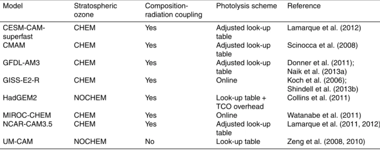
Figure 2 compares vertically resolved ozone decadal trends for the same period, re-gions and seasons, for the ACCMIP multi-model mean and individual models against

20

the Binary Database of Profiles (BDBP version 1.1.0.6) data set, using the so-called Tier 0 and Tier 1.4 data (Bodeker et al., 2013). Tier 0 includes ozone measurements from a wide range of satellite and ground-based platforms, whereas Tier 1.4 is a re-gression model fitted to the same observations. Uncertainty estimates for the BDBP Tier 1.4 trends are from the linear least square fits, as for the observations in Fig. 1.

25

ACCMIP shows most disagreement with the BDBP data in the lower and middle strato-sphere region and best agreement with Tier 1.4 in the upper stratostrato-sphere.

(15)

ACPD

15, 25175–25229, 2015

1850–2100

Title Page

Tables Figures

◭ ◮

Back Close

Full Screen / Esc

Discussion

P

a

per

|

Discussion

P

a

per

|

Discussion

P

a

per

|

Discussion

P

a

per

|

(−0.42, −0.66 and−0.85 % dec−1respectively), the spread of the models at the 95 %

confidence interval stays within the negative range. However, uncertainty estimates

in TCO in the SBUV and BodSci TCO data sets embrace trends of diﬀ_{erent sign}

(−0.65±1.52, and−0.43±2.27 % dec−1 respectively). IGAC/SPARC presents slightly

stronger decadal trends than observations in this region. CMIP5 and CCMVal2

multi-5

model means show slightly stronger decadal trends and agree better with observations than ACCMIP in this region. In terms of absolute values, the spread of the ACCMIP models overlaps the observed TCO for the Hist 2000 time slice, though most models

diﬀ_{er by more than the observational standard deviation (7 out of 8). Biases in TCO}

may be attributed to diﬀ_{erent altitude regions (Fig. 2b). ACCMIP models fail to}

repre-10

sent observed ozone depletion occurring in the lower and middle stratosphere region,

which may be linked to a poor representation of the HOxand NOxcatalytic loss cycles

(e.g. Lary, 1997; Nedoluha et al., 2015).

In the NH midlatitudes (Fig. 1c), ACCMIP simulates smaller decadal trends than

CMIP5 and CCMVal2 (−0.84, −1.36 and −1.38 % dec−1 respectively), though all data

15

sets are at the low end of the observational uncertainties (−1.64–2.45±1.2 % dec−1

respectively). TCO decadal trends for IGAC/SPARC and NOCHEM models, show bet-ter agreement with observations than CHEM models in this region. Due to the BDC,

the abundance of ozone at midlatitudes is aﬀ_{ected by the relatively ozone-rich air}

com-ing from the upper stratosphere over the tropics. The ACCMIP Hist 2000 simulation

20

agrees fairly well with observations in terms of absolute values, however, once again most models diverge by more than the observational standard deviation (7 out of 8). The ACCMIP multi-model mean falls within the BDBP Tier 1.4 uncertainty estimates for most of the lower and middle stratosphere, though simulates weaker ozone depletion in the lower stratosphere and fails to capture a small positive trend between 10–5 hPa,

25

likely associated to tropospheric upwelling and ozone catalytic loss cycle via NOx,

re-spectively (Fig. 2c).

Over the Arctic in boreal spring (Fig. 1e), again the ACCMIP, CMIP5 and

(16)

ACPD

15, 25175–25229, 2015

1850–2100

Title Page

Tables Figures

◭ ◮

Back Close

Full Screen / Esc

Discussion

P

a

per

|

Discussion

P

a

per

|

Discussion

P

a

per

|

Discussion

P

a

per

−2.48 % dec−1 respectively compared to −4.74–5.89±3.4 % dec−1). However, TCO

for Hist 2000 in ACCMIP is in good agreement with observations, with no individual

model diﬀ_{ering by more than the observational standard deviation. In the altitude}

re-gion around 150–30 hPa, the ACCMIP multi-model mean is low biased compared to the BDBP data (Fig. 2e).

5

In the SH midlatitudes (Fig. 1d), ACCMIP simulates TCO decadal trends in better

agreement with observations than in the NH midlatitudes (−2.02 % dec−1compared to

−2.63–3.10±1.3 % dec−1), except for the ACCMIP NOCHEM mean which is

signifi-cantly low biased (−1.14 % dec−1). In terms of absolute values in present-day

condi-tions, most ACCMIP models’ TCO is either high or low biased compared to

observa-10

tions (7 out of 8). The ACCMIP multi-model mean is again low biased compared to the BDBP data set in the altitude range between 150–30 hPa (notice that Tier 1.4 trends are more uncertain in this region), which may be associated to the influence of the

tropics and in-situ HOxcatalytic loss cycle (e.g. Lary, 1997) (Fig. 2d).

Over Antarctica in austral spring (Fig. 1f), ACCMIP CHEM and CMIP5 multi-model

15

means show best agreement compared to observations (−12.87 and−13.92 % dec−1

respectively compared to∼ −13.4–14.3±11 % dec−1), although all data sets fall within

observational uncertainty estimates. IGAC/SPARC ozone data set and NOCHEM

mod-els simulate less ozone depletion in this region (−11.38 and −8.84 % dec−1

respec-tively) than models with interactive chemistry. Although, many ACCMIP models are in

20

good agreement with observations in terms of absolute values for the Hist 2000 time slice, one CHEM model deviates more than the observational standard deviation. AC-CMIP models show fairly good agreement with BDBP Tier 1.4 decadal trends at various

altitude regions, except around 70–30 hPa, likely linked to NOx ozone loss chemistry

associated to stronger temperature trends than observed (see Sect. 5). Biases

rep-25

(17)

ACPD

15, 25175–25229, 2015

1850–2100

Title Page

Tables Figures

◭ ◮

Back Close

Full Screen / Esc

Discussion

P

a

per

|

Discussion

P

a

per

|

Discussion

P

a

per

|

Discussion

P

a

per

|

3.2 Past modelled and future projected total column ozone

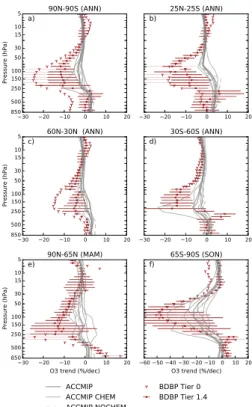
In this section, the evolution of past modelled TCO (from 1850 to 2000) and the sensi-tivity of ozone to future GHG emissions (from 2030 to 2100) under the lower and higher RCPs scenarios are discussed for the regions and seasons presented in the evalua-tion secevalua-tion. In the tropical region, TCO evoluevalua-tion is further analysed by looking at the

5

stratospheric (split into upper and lower regions) and tropospheric columns ozone.

His-torical and future global annual mean of TCO and associated uncertainty (±1 standard

deviation) for the ACCMIP and CMIP5 CHEM models and the IGAC/SPARC data set is given in Table 2.

To probe how diﬀ_{erent emissions of GHG a}ﬀ_{ect stratospheric ozone, we only}

in-10

clude in this section ACCMIP and CMIP5 models with full ozone chemistry (CHEM). In addition, we compare these results with the IGAC/SPARC database, generally used by those models with prescribed stratospheric ozone. Note that tropospheric column

ozone under the RCPs at the end of the 21st century could lead to diﬀ_{erences in TCO}

around 20 DU, due to diﬀ_{erences in ozone precursors emissions (e.g. methane) (Young}

15

et al., 2013a). Again, vertical resolved ozone changes are presented to give insight on the vertical distribution of ozone changes (for the 1850–2100 and 2000–2100 periods). Figure 3 shows, except for the extratropical regions in the SH, an increase in TCO from the pre-industrial period (Hist 1850) to the near-past (Hist 1980) owing to ozone precursors emissions. In the SH extratropical, due to special conditions (e.g. greater

20

isolation from the main sources of ozone precursors and stratospheric cold tempera-tures during austral winter and early spring), there is a decrease in TCO that is

particu-larly pronounced over Antarctica (−12.4 %). Between near-past and present-day (Hist

2000), a period characterised by ODS emissions, the TCO decreases everywhere, with the magnitude being dependent on the region. Thus, the relative change of TCO

be-25

tween the present-day and pre-industrial periods varies across diﬀ_{erent regions, mainly}

(18)

ACPD

15, 25175–25229, 2015

1850–2100

Title Page

Tables Figures

◭ ◮

Back Close

Full Screen / Esc

Discussion

P

a

per

|

Discussion

P

a

per

|

Discussion

P

a

per

|

Discussion

P

a

per

from 2.9 % in the NH midlatitudes and−34.9 % over Antarctica). Notice, however, that

minimal stratospheric ozone depletion occurs before the 1960s.

Future TCO projected for the RCPs 2100 time slices relative to present-day are

aﬀ_{ected by the impact of the Montreal Protocol on limiting ODS emissions, climate}

change and ozone precursors emissions. TCO changes between 2000 and 2100

rel-5

ative to the pre-industrial period for the low and high emission scenarios are in the

range of approximately from−1.2 to 2.0 % in the tropics and 28.3–31.7 % over

Antarc-tica, respectively. Ozone “super-recovery”, defined here as higher stratospheric ozone levels than those during pre-ozone depletion (1850), is found for ACCMIP CHEM mod-els in RCP8.5 2100 in all regions and seasons, with the exception in the tropics and

10

over Antarctica during austral spring. As expected from the above climate impacts, the biggest super-recovery is found, in the order of 12.6 % over the Arctic during boreal spring, and between 3.8–6.5 % at midlatitudes for the RCP8.5 2100 time slice. Similar levels of stratospheric ozone super-recovery are found in the CMIP5 CHEM models. In contrast, the IGAC/SPARC database only projects small super-recovery in the NH

15

polar region and at midlatitudes in the SH. These ozone super-recovery results are consistent with recent findings on stratospheric ozone sensitivity to GHG concentra-tions (Waugh et al., 2009a; Eyring et al., 2010b).

We give special attention to TCO projections in the tropics, since an acceleration of the BDC, due to increases in GHG concentrations would lead to a rise of tropospheric

20

ozone-poor air entering the tropical lower stratosphere (Butchart et al., 2006, 2010, 2011; SPARC-CCMVal, 2010; Eyring et al., 2013). In other words, ozone concentra-tions in the lower stratosphere would decrease with high GHG emissions.

Figure 4 presents upper (>_{10 hPa) and lower (150–15 hPa) stratospheric and}

tro-pospheric columns ozone in the tropics, from the pre-industrial period to the end of

25

the 21st century. Tropospheric column ozone increases with higher ozone precursors emissions during the historical period (1850–2000). Future emissions of ozone

precur-sors (e.g. CO and NOx) are fairly similar among the RCPs scenarios, decreasing to

(19)

ex-ACPD

15, 25175–25229, 2015

1850–2100

Title Page

Tables Figures

◭ ◮

Back Close

Full Screen / Esc

Discussion

P

a

per

|

Discussion

P

a

per

|

Discussion

P

a

per

|

Discussion

P

a

per

|

ception is that the methane burden under the RCP8.5 scenario roughly doubles by the end of the 21st century (Meinshausen et al., 2011). Mainly due to the methane burden and the stratospheric ozone influence via STE, ACCMIP CHEM tropospheric column

ozone change by 2100 relative to present-day is−5.5 and 5.8 DU, for the RCP2.6 and

RCP8.5 scenarios respectively. For both stratospheric columns ozone, there is a small

5

decrease from the pre-industrial period to present-day (−3.2–3.3 DU), which remained

fairly constant by 2030 for both RCPs scenarios. Although ODS concentrations

de-crease during the 21st century, two diﬀ_{erent stories occur in the second half of the}

century. In the upper stratosphere, ozone amounts return to pre-industrial levels under the low emission scenario by 2100. However, RCP8.5 2100 ozone levels relative to

10

present-day increase 8.3 DU, due to a slow down of the ozone catalytic loss cycles, linked to the stratospheric cooling (e.g. Haigh and Pyle, 1982; Portmann and Solomon, 2007; Revell et al., 2012; Reader et al., 2013; Dietmüller et al., 2014). In the lower

stratosphere, ozone levels change little (−0.8 DU) by 2100 relative to the present-day

for the RCP2.6, though decrease by−8.5 DU under the RCP8.5 scenario, likely due to

15

the acceleration of the BDC. In summary, stratospheric column ozone by 2100 remains

fairly similar to the present-day, although diﬀ_{erent stories are drawn in the upper and}

lower stratosphere. RCP2.6 and RCP8.5 2100 TCO relative to pre-industrial period is the result of changes in lower stratospheric and tropospheric columns ozone largely cancelling each other. Therefore, future TCO evolution in the tropics is primarily

deter-20

mined by the upper stratospheric ozone sensitivity to GHG concentrations under the RCPs considered here.

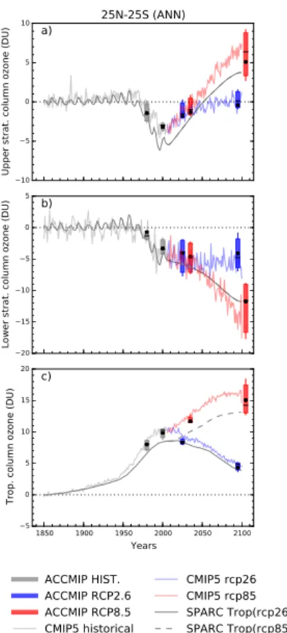
Figure 5 presents vertically resolved ozone change between the Hist 1850 and RCPs 2100 time slices and between the Hist 2000 and RCPs 2100 time slices (top and bottom rows, respectively). In the midlatitudes (Fig. 5b and d), lower stratospheric ozone is

25

(20)

ACPD

15, 25175–25229, 2015

1850–2100

Title Page

Tables Figures

◭ ◮

Back Close

Full Screen / Esc

Discussion

P

a

per

|

Discussion

P

a

per

|

Discussion

P

a

per

|

Discussion

P

a

per

of the upper troposphere-lower stratosphere and the middle and upper stratosphere, relative to pre-industrial (1850) and present-day (2000) levels. We note that climate impact in ozone levels is weaker in the southern than in the northern midlatitudes for

the ACCMIP and CMIP5 multi-model means, likely due to hemispheric diﬀ_{erences in}

STE and ozone flux (Shepherd, 2008), which is in contrast to IGAC/SPARC data set.

5

TCO for the RCP8.5 2100 time slice is 6.9–13.1 % higher than those simulated in the Hist 1850 time slice. While, the RCP2.6 2100 time slice in the northern midlatitudes is similar to present-day levels, in the southern midlatitudes is similar to pre-industrial

levels. This is mainly due to regional diﬀ_{erences in ozone precursors emissions and}

the tropospheric ozone contribution (Fig. 3c and d).

10

Over the Arctic in boreal spring (Fig. 3e), results similar to those in the northern mid-latitudes are found for all models, though higher stratospheric ozone sensitivity to GHG

concentrations lead to approximately two times larger scenario diﬀ_{erences for the 2100}

time slice (37.7 DU between RCP2.6 and RCP8.5). In addition to the RCP8.5 emission scenario, ozone super recovery is also simulated under the RCP2.6 scenario by

AC-15

CMIP and CMIP5 CHEM models. The IGAC/SPARC data set projects similar results to those under the latter scenario. Note that the ACCMIP and CMIP5 multi-model means show a small increase in TCO by 1980 and no significant ozone depletion by 2000 relative to 1850. This is in sharp contrast to the polar region in the SH, which highlights

both regional diﬀ_{erences in ozone precursors sources and atmospheric conditions.}

20

Over Antarctica during austral spring (Fig. 3f), TCO evolution is more isolated from

GHG eﬀ_{ects and ozone precursors than in other regions. In agreement with previous}

studies, ACCMIP and CMIP5 CHEM models project similar values under the lower and higher GHG scenarios (Austin et al., 2010; SPARC-CCMVal, 2010; Eyring et al.,

2013). TCO in the RCPs 2100 time slices remained below 1850s levels (−3.3–6.7 %).

25

(21)

ACPD

15, 25175–25229, 2015

1850–2100

Title Page

Tables Figures

◭ ◮

Back Close

Full Screen / Esc

Discussion

P

a

per

|

Discussion

P

a

per

|

Discussion

P

a

per

|

Discussion

P

a

per

|

small diﬀ_{erences between the above scenarios (e.g. small sensitivity to GHG}

concen-trations). Evolution of stratospheric ozone at high latitudes in the SH, particularly during spring season, has implications over surface climate due to modifications in tempera-ture and circulation patterns.

4 Stratospheric ozone changes and associated climate impacts in the

5

Southern Hemisphere

To probe stratospheric ozone evolution and climate interactions (1850–2100), we first examine simulated stratospheric temperatures in Sect. 4.1. SAM index evolution is presented in Sect. 4.2. Note that ozone loss over the Arctic in boreal spring is only around 25 % of the depletion observed in the Antarctic (see also Fig. 1e), and is not

10

believed to have a significant role in driving NH surface climate (e.g. Grise et al., 2009; Eyring et al., 2010a; Morgenstern et al., 2010).

4.1 Lower stratospheric temperatures changes

Figure 6 shows recent stratospheric temperature decadal trends (1980–2000) in po-lar regions during springtime (March–April–May in the Arctic and October–November–

15

December in the Antarctic). The figure compares temperature in the lower stratosphere (TLS) in the ACCMIP, CMIP5 and CCMVal2 models with observational estimates based on Microwave Sounding Units (MSU) of the Remote Sensing Systems (RSS – sion 3.3) (Mears et al., 2011), the Satellite Applications and Research (STAR – ver-sion 3.0) (Zou et al., 2006, 2009), and the University of Alabama in Huntsville (UAH

20

– version 5.4) (Christy et al., 2003) (Fig. 6a–c). The TLS vertical weighting function from RSS is used to derive MSU temperature from climate models output. Tempera-ture vertical profile decadal trends in the ACCMIP models (Fig. 6b–d) are compared against radiosonde products of the Radiosonde Observation Correction Using Reanal-yses (RAOBCORE – version 1.5), Radiosonde Innovation Composite Homogenization

(22)

ACPD

15, 25175–25229, 2015

1850–2100

Title Page

Tables Figures

◭ ◮

Back Close

Full Screen / Esc

Discussion

P

a

per

|

Discussion

P

a

per

|

Discussion

P

a

per

|

Discussion

P

a

per

(RICH-obs and RICH-tau – version 1.5) (Haimberger et al., 2008, 2012), the Hadley Centre radiosonde temperature product (HadAT2) (Thorne et al., 2005), and the It-erative Universal Kriging (IUK) Radiosonde Analysis Project (Sherwood et al., 2008) (version 2.01).

Over the NH polar cap in boreal spring, although ACCMIP, CMIP5 and CCMVal2

5

models are within observational estimates, all simulates weaker decadal trends (−0.5,

−0.1,−0.4 K dec−1, respectively) than observed (−1.5–1.7±3.4 K dec−1) (Fig. 6a). This

is likely due to the abnormally cold boreal winters in the mid-1990s (i.e. more PSCs for-mation), which resulted in enhanced ozone loss during boreal spring (Newman et al., 2001). Natural variability in models not constrained by observed meteorology is

dif-10

ficult to reproduce (Austin et al., 2003; Charlton-Perez et al., 2010, 2013; Butchart et al., 2011; Shepherd et al., 2014). Moreover, ACCMIP simulations, based on time slice experiments for most models, did not embrace that period, only those boundary conditions for 1980 and 2000 years. This weaker trend on stratospheric temperature is also seen in the vertical profile above around the tropopause (Fig. 6b).

15

Over Antarctica in austral spring, the ACCMIP, CMIP5 and CCMVal2 multi-model

means are in very good agreement (−2.2,−2.5,−1.9 K dec−1, respectively) with

satel-lite measurements (−2.0–2.3±6.4 K dec−1) (Fig. 6c). CHEM models tend to simulate

stronger trends than NOCHEM models, likely due to the fact that the IGAC/SPARC ozone data set is at the lower end of the observational estimates as has been shown

20

in Solomon et al. (2012), Hassler et al. (2013), Young et al. (2014). They argued the importance of the ozone data set for appropriate representation of stratospheric tem-perature, and in turn SH surface climate. Although, large uncertainties exist in this region and period, all ACCMIP individual models fall within the observational error es-timates (Fig. 6d). Note that observational eses-timates are significant at the 95 %

confi-25

dence levels, if year 2000 is removed from the linear fit (−2.95±2.90,−3.02±2.95 and

−3.12±2.87 K dec−1for the RSS, STAR and UAH data sets, respectively), as this year

(23)

ACPD

15, 25175–25229, 2015

1850–2100

Title Page

Tables Figures

◭ ◮

Back Close

Full Screen / Esc

Discussion

P

a

per

|

Discussion

P

a

per

|

Discussion

P

a

per

|

Discussion

P

a

per

|

of ozone in this region (Figs. 1f and 2f). The correlation between stratospheric ozone and temperature trends becomes evident by comparing TCO trends between the Hist 1980 and 2000 time slices and TLS trends for the same period between CHEM and NOCHEM models (i.e. large ozone depletion results in stronger stratospheric cooling trends).

5

Figure 7a depicts SH polar cap TLS long-term evolution (1850–2100) normalised to pre-industrial levels during austral spring. As commented above, stratospheric temper-ature can be perturbed by anthropogenic emissions of ODS and GHG, both having

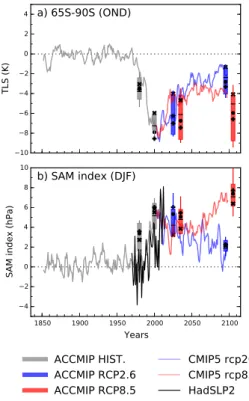
a net cooling eﬀ_{ect. ACCMIP Hist 1980 and 2000 TLS time slices (}₋_{2.5 and}₋_{6.0 K)}

are driven by the combination of ozone depletion and climate change since the

pre-10

industrial period. In future projections, ozone recovery and GHG concentrations are

ex-pected to have an opposite eﬀ_{ect on stratospheric temperatures. The slightly increased}

of the TLS by 2030 in the RCPs time slices relative to present-day, is very similar be-tween the lower and higher RCPs emission scenarios (0.9 and 0.4 K, respectively). By the end of the 21st century, the projected TLS under the RCP2.6 scenario returns

15

to Hist 1980 levels, whereas it remains fairly unchanged under the RCP8.5 scenario

relative to 2030. These two diﬀ_{erent stories suggest a key role of GHG concentration}

in the second half of the century, with significant implications for many aspects of the SH surface climate as reported previously (McLandress et al., 2011; Perlwitz, 2011; Polvani et al., 2011); see Sect. 4.2 and Thompson et al. (2011) and Previdi and Polvani

20

(2014) for a comprehensive review.

4.2 Southern Annular Mode evolution

The SAM index is defined as per Gong and Wang (1999), by subtracting the zonal

mean sea level pressure (SLP) at 65◦_{S latitude from the zonal mean SLP at 40}◦_S

latitude from monthly mean output. The SAM index is a proxy of variability in the jets

25

(24)

ACPD

15, 25175–25229, 2015

1850–2100

Title Page

Tables Figures

◭ ◮

Back Close

Full Screen / Esc

Discussion

P

a

per

|

Discussion

P

a

per

|

Discussion

P

a

per

|

Discussion

P

a

per

Figure 7b shows SAM index long-term evolution (1850–2100) normalised to 1850 levels during austral summer. Observational estimates based on the Hadley Centre Sea Level Pressure data set (HadSLP2) are shown from 1970 to 2012. The AC-CMIP multi-model mean shows a positive trend between Hist 1980 and 2000 time

slices (1.27 hPa dec−1), coinciding with the highest ozone depletion period. Within

un-5

certainty, this is weaker than observational estimates (2.2±1.1 hPa dec−1). ACCMIP

CHEM and NOCHEM models show similar SAM index trends, although the latter presents weaker TLS trends (see Fig. 6c). As seen in Fig. 7a for the TLS in austral spring, by 2030 for both RCPs scenarios the ACCMIP multi-model mean shows a slight decrease in the SAM index relative to Hist 2000.

10

Two diﬀ_{erent stories are drawn from 2030 to 2100. The SAM index simulated}

un-der the RCP2.6 scenario tends to return to “normal” levels (−0.4 hPa dec−1), as ODS

concentrations and GHG emissions decrease during the second half of the century. In contrast, under the RCP8.5 scenario GHG concentrations increase, resulting in a

pos-itive trend of the SAM index (0.3 hPa dec−1). By using a paired sample Student’st_test,

15

we find that SAM index changes between Hist 2000 and 2100 relative to Hist 1850, are significant for the RCP2.6 at the 5 % level, although is not significant for the RCP8.5. CMIP5 multi-model mean shows better agreement with observations during the record

period (2.1 hPa dec−1) than ACCMIP. During the second half of the 21st century (2030–

2100), however, the CMIP5 multi-model mean shows consistent projections with the

20

latter (−0.4 and 0.4 hPa dec−1for RCP2.6 and RCP8.5, respectively).

5 Discussion

TCO trends in ACCMIP models compare favourably with observations, however, ozone trends in the tropical lower stratosphere are low biased (e.g. weaker ozone depletion). It has been argued that tropical upwelling (or the BDC) is the main driver in this

re-25

(25)

ACPD

15, 25175–25229, 2015

1850–2100

Title Page

Tables Figures

◭ ◮

Back Close

Full Screen / Esc

Discussion

P

a

per

|

Discussion

P

a

per

|

Discussion

P

a

per

|

Discussion

P

a

per

|

observed BDC and its seasonal cycle (Fu et al., 2010; Young et al., 2011) are poorly constrained in modelling studies (e.g. Butchart et al., 2006, 2010; Garcia and Ran-del, 2008). This is important since ozone depletion determines to a large extent the temperatures in the lower stratosphere (e.g. Polvani and Solomon, 2012) (note that temperature trends in this region are low biased in ACCMIP models compared to

ob-5

servations, not shown), and the latter triggers significant feedbacks in climate response (Stevenson, 2015). Models with less ozone depletion in the tropical lower stratosphere may have stronger climate sensitivity (Dietmüller et al., 2014; Nowack et al., 2015).

Long-term TCO changes relative to Hist 1850 in the ACCMIP models considered in this study, are least consistent for Hist 2000 in the Antarctic springtime (i.e. the period

10

with large ozone losses) and for RCP8.5 2100 in general. The latter is likely linked to sensitivity of ozone to future GHG emissions uncertainty (i.e. various direct and indirect

processes aﬀ_{ecting ozone amounts in the troposphere and the stratosphere). For}

ex-ample, CO₂and methane mixing ratios increase by more than 3 and 4 times in RCP8.5

2100 relative to the pre-industrial period, respectively. Nevertheless, the ACCMIP and

15

CMIP5 multi-model means, show consistent RCP8.5 2100 projections. Although TCO changes are relative to the Hist 1850, a period without direct measurements (e.g. es-timates with large uncertainties), ACCMIP models show good agreement compared to other time slices. For example, the interquartile range (central 50 % of the data) varies approximately 3–8 % of the corresponding mean value across the regions and seasons

20

considered here.

Stratospheric ozone has been shown to be asymmetrical over the SH polar cap (Grytsai et al., 2007). Prescribing zonal mean ozone fields in CCMs may have im-plications on SH climate (e.g. Crook et al., 2008; Gillett et al., 2009), particularly in early spring stratospheric temperatures (September–October) and, though less

pro-25

(26)

ACPD

15, 25175–25229, 2015

1850–2100

Title Page

Tables Figures

◭ ◮

Back Close

Full Screen / Esc

Discussion

P

a

per

|

Discussion

P

a

per

|

Discussion

P

a

per

|

Discussion

P

a

per

showed that NOCHEM models simulated both weaker springtime TLS negative trends over the Antarctic compared to observational estimates, and stronger positive trends in the near-future compared to CHEM models. In addition, Young et al. (2014) find large

diﬀ_{erences in SH surface climate responses when using di}ﬀ_{erent ozone data sets.}

AC-CMIP CHEM and NOCHEM models show most disagreement on SAM index trends in

5

the near-future, period with relatively strong ozone depletion (>_{Hist 1980). The former}

projects negligible trends compared to−0.57 hPa dec−1and three times weaker

nega-tive trends than the latter, for the RCP2.6 and RCP8.5 respecnega-tively. This is consistent with CHEM and NOCHEM TLS springtime trends in this period and region. Never-theless, ACCMIP models participating in this study agree with previous observational

10

(e.g. Thompson and Solomon, 2002; Marshall, 2003, 2007) and modelling studies (e.g. Gillett and Thompson, 2003; Son et al., 2008, 2010, 2009; Polvani et al., 2010, 2011; Arblaster et al., 2011; McLandress et al., 2011; Gillett and Fyfe, 2013; Keeble et al., 2014) on the SH surface climate response, measured here using the SAM index.

6 Summary and conclusions

15

This study has analysed stratospheric ozone evolution from 1850 to 2100 from a group of chemistry climate models with either prescribed or interactively resolved time-varying ozone in the stratosphere and participated in the ACCMIP activity (8 out of 15 models). We have evaluated TCO and vertically resolved ozone trends between 1980 and 2000, and examined past and future ozone projections under the low and

20

high RCPs future emission scenarios (RCP2.6 and RCP8.5, respectively). Finally, we have assessed TLS and temperature profile trends at high latitudes in the recent past, and analysed TLS and SH surface climate response (diagnosed using the SAM index), from the pre-industrial period to the end of the 21st century.

Within uncertainty estimates, the ACCMIP multi-model mean TCO compares

25