NUMERICAL SIMULATION OF SHALLOW WATERS EFFECTS ON SAILING SHIP "MIRCEA" HULL

NUMERICAL SIMULATION OF SHALLOW WATERS EFFECTS ON SAILING SHIP

"MIRCEA" HULL

Petru Sergiu ȘERBAN1

1

PhD Student, Department of Navigation and Naval Transport, “Mircea cel Batran” Naval Academy, Constanța, Romania, sergiu.serban@anmb.ro

Abstract: CFD techniques for studying the influence of hydrodynamic forces on ships are increasingly used in the maritime community, including the study of ship to bank, ship to ship and ship to bottom interaction in shallow waters. The paper aims to the process and selection of appropriate methods for creating the geometry, mathematical model setup and simulation using Ansys CFD CFX program. CFD simulations were conducted to observe the effects of limited depth on sailing ship ”Mircea” hull in two domains, one with a depth of 20.35 m and the other with a depth 6.85 m.

Keywords: CFD, simulation, mesh, hull, depth.

INTRODUCTION

Evaluation of ship hydrodynamic parameters began to gain importance with the advent of power-driven vessels in the nineteenth century. The latest approach is Computational Fluid Dynamics (CFD) numerical method, which required for its development mutual cooperation of several disciplines such as mathematics, physics and information technology. CFD simulations have gained popularity in the '90s and replace experiments in many fields today [1].

CFD represents the computer technology to analyze fluid handling systems including heat transfer and associated phenomena through computer-based simulation methods. This technology uses numerical methods and algorithms to solve equations describing fluid flow and heat transfer. Computers are used for data preparation, domain construction and meshing, calculating the numerical solution of equations and analyze the results.

CFD techniques for studying the influence of hydrodynamic forces on ships are increasingly used in the maritime community, including the study of ship to bank, ship to ship and ship to bottom interaction in shallow waters [2].

As the ship enters in shallow waters, a series of changes occur due to interaction between ship and seabed. Therefore, the restricted space between the hull and the sea/river bottom causes an increase of the potential speed flow. The pressure drop around the hull results in a reduction of buoyancy and center of buoyancy modification. Thus, the ship is affected by an increase in draft and trim change.

The study presented in this paper aims to the process and selection of appropriate methods for creating geometry, mathematical model setup and simulation using Ansys CFD CFX program that uses a 3D solver based on the Finite Volume Method.

Having the blueprints of sailing ship “Mircea”, the hull was geometrically shaped up to the 7m water line, and then there were defined two domains with a depth of 20.35 m and 6.85 m to study the effects on the hull produced by depth. These effects relate mainly to change in pressure, velocity, forces and torques on the body.

GEOMETRY MODELING

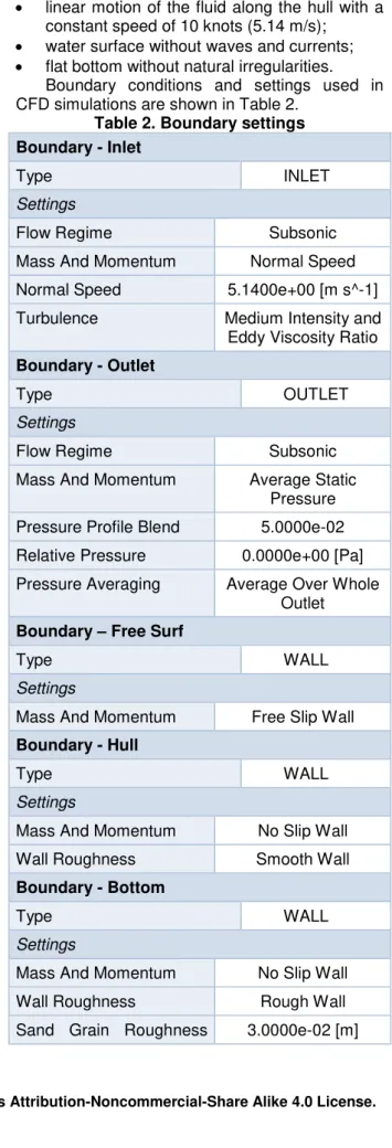
The simulation domain should be large enough horizontally to prevent the influence of boundary flow, but the maximum size of the field is limited by the performance of the computer. CFD simulation was conducted in two domains, one with a depth of 20.35 m and the other with a depth 6.85 m.

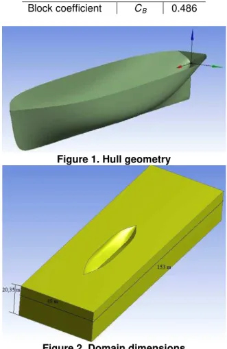
Trial runs in towing tanks to determine hull drag can be replaced with CFD techniques with the advantage that they can be applied directly to the prototype. The first step is the preparation of the hull CAD geometry. This was done based on the data from Table 1. The final 3D form of sailing ship “Mircea” hull used for the analysis is shown in Figure 1.

Table 1. Hull geometry parameters Water line length LWL[m] 62.061 Water line breadth BWL [m] 12.00

Height D [m] 7.00

Draft T [m] 5.35

Displacement ∆ [t] 1984.2

97 DOI: 10.21279/1454-864X-16-I2-015

Block coefficient CB 0.486

Figure 1. Hull geometry

Figure 2. Domain dimensions

The environment in which the ship is moving is known as the domain. The dimensions of the area (length, width, depth) surrounding the ship are shown in Figure 2.

COMPUTATIONAL DOMAIN MESHING

Dividing the computational domain into a number of cells is called meshing. Special care should be given when creating the mesh because a poor quality has a negative effect on solution convergence and confidence in the results.

To numerically analyze the flow, the physical domain is meshed in cells. The flow variables are associated with each flow cell (element) in the mesh. In both cases, the tetrahedron method was chosen for meshing throughout the entire fluid domain. In the first case (h = 20.35 m) there were a number of 402437nodes and 258950 elements, and in the second case were obtained 242665 nodes and 147771 elements.

This model uses the finite element method with a second order meshing. Compared with a first order meshing, it offers a greater convergence and a higher accuracy of the mesh.

Figure 3 shows the mesh obtained for the first domain studied.

Figure 3. Domain mesh

Mesh generation of the fluid domain was done in three steps:

• it was created a free mesh on all surfaces to automatically determine the appropriate number of divisions on each side faces using Face Meshing function;

• then the mesh was refined using Patch Conforming, Tetrahedrons function;

• there have been added inflation layers around the hull using Inflation function to capture the flow in the boundary layer.

To measure the quality of generated mesh there were used Skewness and Orthogonal quality functions from Mesh Statistics, which are among the most important methods for determining the quality of a mesh.

It is generally recommended to maintain minimum orthogonality higher than 0.15 and maximum asymmetry (skewness) less than 0.95. Cells or items that do not meet these conditions can lead to incorrect results of the simulation. However, these are general guidelines and depend on the type of the problem or location of these cells. MATHEMATICAL MODEL AND SOLVER

To derive the equations of fluid motion, one has to know the change rate of fluid properties φ per unit mass and unit volume. This domain is completely described by the density ρ, speed U, pressure p and viscosity μ. The rate of change in the properties of a fluid φ per unit volume is given by (1):

( )

=

0

∇

+

∂

∂

U

t

ρ

ρ

(1). The shear stresses from the momentum equations can be related to linear deformation rates of the fluid element, which is expressed by velocity components. For an isotropic Newtonian fluid, the relationship between shear stress and deformation rate is given by the following equation:

98 DOI: 10.21279/1454-864X-16-I2-015

z x y x y z y z x zz zy zx yz yy yx xz xy xx p p p p p p ε ϑ ϑ ϑ ε ϑ ϑ ϑ ε µ τ τ τ τ τ τ ⋅ + − = 2 0 0 0 0 0 0 (2).

This is the momentum equations in the most convenient form for finite volume method. In some sources, Navier-Stokes equations are associated with momentum equations and continuity equation system.

The simulation was performed based on RANSE method for incompressible viscous flow, which is derived from averaging Navier-Stokes equations. Mediation leads to a set of partial differential equations called Reynolds averaged Navier-Stokes equations (RANSE) which is the main mean in the CFD arsenal methods used today for calculating turbulent flows [5].

In this paper, viscous flow along the ship's hull is supposed to be incompressible and the numerical problem is described by RANS equations.

Turbulence models with two equations are some of the most common types of turbulence models. Models, such as k-ε and k-ω, have become standard models and are used often for various types of engineering problems. Regarding the flow along a ship hull, the literature states that the k-ω Shear Stress Transport turbulence model, which is a combination of k-ε and k-ω models, simulates the flow with greater accuracy compared to other models of turbulence; therefore, it was used also in this study [6]. The two equations of the model are:

• transport equation for turbulence kinetic energy k:

( )

(

)

j k j i i S Y G x k x ku x k

t _+ − +

     ∂ ∂ Γ ∂ ∂ = ∂ ∂ + ∂

∂ _{ρ ρ}

(3) • transport equation for specific dissipation ω:

( )

(

)

x x u x

t j j

i i + + − +         ∂ ∂ Γ ∂ ∂ = ∂ ∂ + ∂ ∂ (4). K-ω SST model is the most advanced model of isotropic turbulence models with two equations currently available. Meanwhile, it has been validated in a significant degree, for a sufficiently wide range of flows. So, for most applications, this model is the recommended choice [3].

The boundaries defining and separating fluid zones can be of various types that depend on the setting of the problem and the role played by these limits in solution. The most common types are wall, input, output, symmetry, periodic and interface.

When defining the mathematical model there were made the following assumptions:

• linear motion of the fluid along the hull with a constant speed of 10 knots (5.14 m/s);

• water surface without waves and currents; • flat bottom without natural irregularities.

Boundary conditions and settings used in CFD simulations are shown in Table 2.

Table 2. Boundary settings Boundary - Inlet

Type INLET

Settings

Flow Regime Subsonic

Mass And Momentum Normal Speed

Normal Speed 5.1400e+00 [m s^-1]

Turbulence Medium Intensity and Eddy Viscosity Ratio

Boundary - Outlet

Type OUTLET

Settings

Flow Regime Subsonic

Mass And Momentum Average Static Pressure

Pressure Profile Blend 5.0000e-02

Relative Pressure 0.0000e+00 [Pa]

Pressure Averaging Average Over Whole Outlet

Boundary – Free Surf

Type WALL

Settings

Mass And Momentum Free Slip Wall

Boundary - Hull

Type WALL

Settings

Mass And Momentum No Slip Wall

Wall Roughness Smooth Wall

Boundary - Bottom

Type WALL

Settings

Mass And Momentum No Slip Wall

Wall Roughness Rough Wall

Sand Grain Roughness 3.0000e-02 [m]

99 DOI: 10.21279/1454-864X-16-I2-015

Height

Boundary - Lateral walls

Type WALL

Settings

Mass And Momentum Free Slip Wall

RESULTS AND DISCUSSIONS

Calculations were performed with Ansys CFX solver. Turbulent flow was simulated by solving the Reynolds averaged Navier - Stokes equations for incompressible flow. Velocity field is obtained from the momentum conservation equations and the pressure field is extracted from the condition of mass conservation or continuity equation converted into a pressure equation. In turbulent flow cases, additional transport equations for variables modeling are discredited and solved using the same principles [4].

All calculations presented in this study were made for the body without appendages of sailing ship “Mircea”.

CFX solver converts the differential equations defined in the mathematical model into a set of algebraic equations. Solving these equations there are obtained values for u, v, w, p, k, ω in the center of each cell of the domain. In the first case (h = 20.35 m), the mesh contains about 260000 cell. The total number of unknowns and implicit algebraic equations is 260000 * 6 = 1.56 million. This huge set of algebraic equations is solved by an iterative process. The analysis is transient, lasting a total of 100 s and 0.5 s steps, each step having 5 iterations.

During post processing, the desired information is extracted from the data set generated by the CFD code. Versatile viewing functions are an advantage of CFD packages. After analysis, the results can be represented in tables, graphics or contours. Thus, pressure profiles, forces acting on the hull and speed profiles in different sections were determined.

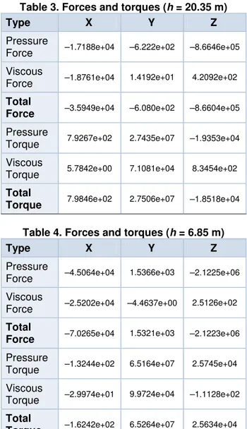
In Tables 3 and 4 are given the pressure, viscosity and total forces and torques acting on body in considered cases. The resultant force in X direction is the drag of the vessel, in Y direction is the drift and in Z direction is the vertical hydrodynamic force which causes the vessel to sink due to the interaction with the bottom.

Table 3. Forces and torques (h = 20.35 m)

Type X Y Z

Pressure

Force ‒1.7188e+04 ‒6.222e+02 ‒8.6646e+05

Viscous

Force ‒1.8761e+04 1.4192e+01 4.2092e+02

Total

Force ‒3.5949e+04 ‒6.080e+02 ‒8.6604e+05

Pressure

Torque 7.9267e+02 2.7435e+07 ‒1.9353e+04

Viscous

Torque 5.7842e+00 7.1081e+04 8.3454e+02

Total

Torque 7.9846e+02 2.7506e+07 ‒1.8518e+04

Table 4. Forces and torques (h = 6.85 m)

Type X Y Z

Pressure

Force ‒4.5064e+04 1.5366e+03 ‒2.1225e+06

Viscous

Force ‒2.5202e+04 ‒4.4637e+00 2.5126e+02

Total

Force ‒7.0265e+04 1.5321e+03 ‒2.1223e+06

Pressure

Torque ‒1.3244e+02 6.5164e+07 2.5745e+04

Viscous

Torque ‒2.9974e+01 9.9724e+04 ‒1.1128e+02

Total

Torque ‒1.6242e+02 6.5264e+07 2.5634e+04

These results were post-processed as hull contours shown in Figure 4. It is noted that in the second case, all the forces acting on the hull are higher than in the first situation due to reduced depth. Thus, the maximum drag value increases from 2925 N to 2986 N, transverse forces acting on the hull are stronger and the maximum vertical force drops from ‒4131 N to ‒10780 N, which proves that shallow depth produces hydrodynamic effects on the hull.

Pressure variation on hull is shown in Figure 5, where it can be seen a normal distribution for a ship’s body, with two positive pressure zones in the bow and stern of the ship and a negative pressure zone at the bottom, along the hull.

100 DOI: 10.21279/1454-864X-16-I2-015

Figure 4. Vertical forces contours for h = 20.35 m (top) and h = 6.85 m (bottom)

Figure 5. Pressure variation for h = 20.35 m

Speed variation of the fluid along the hull is shown in Figure 6. As expected, one can see the potential increase in flow rate due to ship – bottom interaction. Thus, the fluid particle velocity under the hull increases, reaching a maximum of 5.65 m/s in the first case, and 6.13 m/s in the second case, unlike the initial fluid velocity 5.14 m/s (10 knots).

Figure 5. Speed variation for h = 20.35 m (top) and h = 6.85 m (bottom)

To verify that the model used is good and the solution converges, the total mass of fluid at inlet must be equal to the mass at outlet. This is shown in Table 5.

Table 5. Mass flow

Case Location Mass Flow

h = 20.35 m inlet 5.0078e+06 outlet ‒5.0079e+06

h = 6.85 m inlet 1.6866e+06 outlet ‒1.6866e+06

The numerical convergence adopted for these calculations was the criteria of reducing the maximum difference between consecutive iterations for velocity components and pressure below a value of 10‒4. Residuals range between 10‒4 and 10‒7 during the 5 iterations time step. A comparative study by refining the mesh is important in the verification stage. A finer mesh can yield more precise results of the model, but consume more computing resources. The user must find a balance between mesh size and consumption of computing resources.

Regarding validation, currently there are no experimental data carried on board sailing ship “Mircea” performed to validate simulation results.

101 DOI: 10.21279/1454-864X-16-I2-015

CONCLUSIONS

The paper presents the steps of a CFD numerical simulation conducted to observe the effects of limited depth on sailing ship ”Mircea” hull. These steps relate primarily to the construction of the geometric model, mesh generation, mathematical model and results post-processing.

The velocity variation along the hull was as expected, with a potential increase in the flow rate under the hull, due to the interaction between the hull and the bottom. Also, pressure variation on hull is normal for a ship body, with positive pressure zones in the fore and aft and a negative pressure at the bottom of the hull, along the body.

The solution obtained had converged as the velocity components and pressure residuals drop below the value 10‒4. Therefore, the method used is good and the solution is verified by the compliance with mass conservation law.

Regarding validation, currently there are no experimental data carried on board sailing ship “Mircea” to validate simulation results.

Future development includes comparing simulation results obtained with different RANSE methods. These comparisons will be made for various speeds and depths, but also for more refined meshes.

BIBLIOGRAPHY

[1] Benes P., Kollarik R., Preliminary Computational Fluid Dynamics (Cfd) Simulation Of Eiib Push Barge In Shallow Water, Scientific Proceedings 2011, Faculty of Bechanical Engineering, STU in Bratislava, vol. 19, 2011, pp. 67 – 73.

[2] Nakisa M. ș.a., Three-dimensional numerical analysis of restricted water effects on the flow pattern around hull and propeller plane of LNG ship, International Journal of Mechanics, Issue 3, Vol. 7, 2013, pp. 234 – 241.

[3] Maimun A., ș.a., Assessment of Ship-Bank Interactions on LNG Tanker in Shallow Water, Department of Marine Technology, University Technology Malaysia, Johor Bahru, Malaysia, The 6th Asia-Pacific Workshop on Marine Hydrodymics-Phydro 2012 Malaysia, September 3-4, 2012.

[4] Ristea M., Popa A., Cotorcea A., RANSE simulation for a two DoF ship model, “Mircea cel Bătrân” Naval Academy Scientific Bulletin, Vol. XVIII, issue 2, 2015, pp. 148 – 152.

[5] Ristea M., Popa A., Neagu D., CFD modelling of a 5 bladed propeller by using the RANSE approach, “Mircea cel Bătrân” Naval Academy Scientific Bulletin, Vol. XVIII, issue 2, 2015, pp. 153 – 158.

[6] Toma A., Scurtu I., Ansys and Autoship numerical simulation for ship model, Constanța Maritime University Annals, Year XVII, vol. 25, Ed. Nautica Constanța, 2016, pp. 155-158.

102 DOI: 10.21279/1454-864X-16-I2-015