❊♥s❛✐♦s ❊❝♦♥ô♠✐❝♦s
❊s❝♦❧❛ ❞❡
Pós✲●r❛❞✉❛çã♦
❡♠ ❊❝♦♥♦♠✐❛
❞❛ ❋✉♥❞❛çã♦
●❡t✉❧✐♦ ❱❛r❣❛s
◆◦ ✼✶✶ ■❙❙◆ ✵✶✵✹✲✽✾✶✵
●❛✐♥s ❢r♦♠ tr❛❞❡ ❛♥❞ ♠❡❛s✉r❡❞ t♦t❛❧ ❢❛❝t♦r
♣r♦❞✉❝t✐✈✐t②
✱
❖s ❛rt✐❣♦s ♣✉❜❧✐❝❛❞♦s sã♦ ❞❡ ✐♥t❡✐r❛ r❡s♣♦♥s❛❜✐❧✐❞❛❞❡ ❞❡ s❡✉s ❛✉t♦r❡s✳ ❆s
♦♣✐♥✐õ❡s ♥❡❧❡s ❡♠✐t✐❞❛s ♥ã♦ ❡①♣r✐♠❡♠✱ ♥❡❝❡ss❛r✐❛♠❡♥t❡✱ ♦ ♣♦♥t♦ ❞❡ ✈✐st❛ ❞❛
❋✉♥❞❛çã♦ ●❡t✉❧✐♦ ❱❛r❣❛s✳
❊❙❈❖▲❆ ❉❊ PÓ❙✲●❘❆❉❯❆➬➹❖ ❊▼ ❊❈❖◆❖▼■❆ ❉✐r❡t♦r ●❡r❛❧✿ ❘✉❜❡♥s P❡♥❤❛ ❈②s♥❡
❉✐r❡t♦r ❞❡ ❊♥s✐♥♦✿ ❈❛r❧♦s ❊✉❣ê♥✐♦ ❞❛ ❈♦st❛
❉✐r❡t♦r ❞❡ P❡sq✉✐s❛✿ ▲✉✐s ❍❡♥r✐q✉❡ ❇❡rt♦❧✐♥♦ ❇r❛✐❞♦
❉✐r❡t♦r ❞❡ P✉❜❧✐❝❛çõ❡s ❈✐❡♥tí✜❝❛s✿ ❘✐❝❛r❞♦ ❞❡ ❖❧✐✈❡✐r❛ ❈❛✈❛❧❝❛♥t✐
✱
●❛✐♥s ❢r♦♠ tr❛❞❡ ❛♥❞ ♠❡❛s✉r❡❞ t♦t❛❧ ❢❛❝t♦r ♣r♦❞✉❝t✐✈✐t②✴ ✱ ✕ ❘✐♦ ❞❡ ❏❛♥❡✐r♦ ✿ ❋●❱✱❊P●❊✱ ✷✵✶✶
✶ ♣✳ ✲ ✭❊♥s❛✐♦s ❊❝♦♥ô♠✐❝♦s❀ ✼✶✶✮ ■♥❝❧✉✐ ❜✐❜❧✐♦❣r❛❢✐❛✳
❊♥s❛✐♦s ❊❝♦♥ô♠✐❝♦s ❞❛ ❊P●❊✴❋●❱ ✭■❙❙◆✿ ✵✶✵✹✲✽✾✶✵✮ ♥✳ ✼✶✶
●❛✐♥s ❢r♦♠ tr❛❞❡ ❛♥❞ ♠❡❛s✉r❡❞ t♦t❛❧ ❢❛❝t♦r
♣r♦❞✉❝t✐✈✐t②
Gains from trade and measured total factor
productivity
Pedro Cavalcanti Ferreira
yEPGE - Fundação Getulio Vargas
Alberto Trejos
zINCAE
May 31, 2010
Abstract
We develop and calibrate a model where di¤erences in factor en-dowments lead countries to trade di¤erent goods, so that the existence of international trade changes the sectorial composition of output from one country to another. Gains from trade re‡ect in total factor produc-tivity. We perform a development decomposition, to assess the impact of trade –and barriers to trade– on measured TFP. In our sample, the median size of that e¤ect is about 6.5% of output, with a median of 17% and a maximum of 89%. Also, the model predicts that changes in the terms of trade cause a change of productivity, and that e¤ect has an average elasticity of 0.71.
The authors would like to thank Samuel Pessôa, Tim Kehoe, two anonymous referees and seminar participants at EPGE/FGV, Universidade do Minho, the Society of Economic Dynamic 2008 meeting, the Lacea-Lames 2009 meeting and the 2009 European Meeting of the Econometric Society for useful suggestions and comments. Ferreira would like to thank CNPq/INCT and Faperj for the support.
1
Introduction
A large literature (e.g., Mankiw, Romer and Weil (1992), Prescott (1998), Klenow and Rodriguez-Clare (1997), Caselli (2005) among many) has stud-ied the cross-country di¤erences in total factor productivity, that is, those di¤erences in output per-capita that cannot be explained by corresponding di¤erences in available inputs. In these exercises, it is assumed that the tech-nology that transforms inputs into output is the same across countries, except for a single TFP coe¢cient that changes the e¤ectiveness of the overall produc-tion process, but does not change the way di¤erent inputs interact with each other. The functional forms used in these analyses are chosen assuming that countries do not trade with each other, and are calibrated using parameters that give a good …t to the data of developed nations.
In this paper, we quantify the impact of international trade on Total Factor Productivity (TFP). Trade leads to a more e¢cient allocation of resources across sectors, and thus may a¤ect aggregate productivity even if sectorial productivities are not allowed to di¤er across countries. Since barriers to trade do vary signi…cantly, the degree to which gains from trade are exploited may be a relevant component in explaining cross-country TFP di¤erences.
Here, we use a one-period version of the model developed in Ferreira and Trejos (2006), with the adjustments made necessary by the cross-country data analysis that follows. The equilibrium of that model under autarky is homeo-morphic to the standard model used in most development accounting exercises, so comparison is convenient. The simplest way of formulating this model is to interpret the traded goods as inputs in the production function of a …nal non-tradeable good, but it is not the fact that these are intermediate goods that matters, but rather that there is a sectorial allocation problem that trade barriers may distort. By construction, this model predicts that trade will be of little importance for rich countries, but for a poor country the model pre-dicts that trade induces a sizeable gain in TFP, which increases with trade liberalization and with the terms of trade1.
We calibrate this model and apply it to a large sample of developing coun-tries, to assess the quantitative importance of the e¤ects mentioned above. Because countries reap at least some of these bene…ts from trade, the TFP di¤erences between rich and poor countries that are estimated with our model are larger than those emerging from more conventional output decompositions, which are performed assuming a closed economy. For the country in our data-base with the lowest capital endowment per worker, Uganda, our calibrated model estimates that free trade could increase output by 89:8% compared to autarky; in other words, the raw productivity di¤erence relative to the US is much larger than conventional measurements (which would impute those gains from trade as productivity) would deliver. The assessed gains from trade for other African nations (Congo, Mozambique and Rwanda, among others) range between 50% and 62% of productivity; for several Asian countries, around
15%. Of course, many countries waste a good part of these gains through protectionism. We estimate that in 1985 Bangladesh and India, who should have enjoyed gains from trade to the tune of 1=3 of GDP due to their capital scarcity, wasted most or all those gains with average tari¤s at prohibitive levels over 90%.
Because countries can pick very di¤erent trade policies, the model adds another dimension that can explain the behavior of TFP residuals. We do not have comparable cross-country data for transportation costs, non-tari¤ barriers, and other phenomena that reduce the incentives to international ex-change. But looking at data on tari¤s we …nd that for some poor nations, those barriers alone are large enough to account for large di¤erences in
ductivity. Due to the nature of the trade problem, the same tari¤s would have a di¤erent cost in di¤erent countries, because both the potential gains from trade and the distortionary e¤ect of policy vary with the capital-labor ratio. For instance, in 1985 Brazil and Benin had similar nominal tari¤ rates, under which poorer Benin realized almost all its (large) potential gains from trade, while the wealthier Brazil lost most of its (proportionally smaller) bene…ts.
Other authors have pursued to quantify the relationship between trade and productivity, although emphasizing di¤erent transmission mechanisms. For instance, Eaton and Kortum (2002) develop a model where TFP is speci…c to each country and industry, so trade allows countries to allocate more resources to the industries that have drawn high productivities. Using a similar model, Lucas and Alvarez (2008) estimated that a country with 1% of world GDP would gain from openness to trade up to 41%in productivity. Using a similar model, Rodriguez-Clare (2007) obtains similar estimates, which become much higher if openness involves not only the possibility to exchange goods, but also fosters the di¤usion of ideas.
An open economy with barriers to trade is one of the simplest examples of resource misallocation in a sectorial problem, and thus the mechanism de-scribed here is related to a recent literature that emphasizes ine¢ciencies in the composition of output as a means to explain di¤erences in TFP. For in-stance, Restuccia and Rogerson (2008) show that policies that distort prices faced by individual producers can lead to 50 percent decreases in measured TFP. Likewise, Hsieh and Klenow (2007) use a standard model of monopolistic competition with heterogeneous …rms to measure the impact on productivity of the resource misallocation caused by distortions across …rms. They …nd that the removal of these distortions could boost TFP in India by as much as 60%.
de-scribes an empirical link of this sort. Kehoe and Ruhl (2008) show that one can explain this empirical link with a standard macro model only under very limited speci…cations both of the theory and of the measurement, and thus pose that this strong empirical relationship is a puzzle. Our model can help explain this puzzle, since it predicts –in a manner that is quite natural within a Hecksher-Ohlin framework– that an improvement in terms of trade simply allows a better sectorial composition, that yields more …nal output out of the same inputs. Under our calibration, for a very capital-poor country a 10%
gain in the terms of trade yields a5:7% gain in TFP, and these e¤ects can be larger depending on factor endowments and trade policies2.
In Section 2 we describe and solve the model, and in Section 3 we describe the data and calibration. In Section 4, we present the results and Section 5 concludes.
2
The model
We model the world as a collection of small economies that trade with a much larger and wealthier country. The asymmetry in sizes is such that –for all practical purposes– the autarkic domestic prices in the big country are the international prices, and the small countries are price takers. The picture in our mind is that the big economy is the US (or perhaps the US plus the EU). We focus our attention on the equilibrium allocation in the other countries.
There are three goods in these economy: two non-storable, tradable in-termediate products, A and B, and a …nal good, Y, which presumably can be consumed or invested (but we do not look at consumption or investment decisions here), and that cannot be traded. Each good is produced, by a large number of small, competitive …rms, using technologies that have constant re-turns to scale.
There are also two factors of production in this economy: labor in e¢cient
2Other possible explanations are …nancial market frictions (Mendoza, 2006), labor
units L and physical capital K. Labor and capital are used in producing A
and B, and these in turn are used to produce Y. The endowment of labor, measured in e¢ciency units, is given by:
L=N h=N e s;
where N is the number of workers, h represents e¢ciency-units of labor per worker ands stands for schooling. The production functions of A and B are:
A = K a
A L
1 a
A
B = K a
B L
1 b
B :
Without loss of generality, A is labor-intensive: a < b. We use B as
nu-meraire, and the relative prices of A and Y in terms ofB are denoted p and .
Because A and B are tradable, the amounts of them that are used in the production of the …nal good (denoted a and b) may di¤er from the amounts produced (denoted A and B). Total output ofY is given by:
Y = a b1
: (1)
All markets are perfectly competitive; in the case of A and B, these are not domestic but rather global markets, from which local Y producers can import provided they pay an ad-valorem tari¤ . The rate captures all the (policy or non-policy induced) costs of bringing goods into the local market.
We denote k =K=L in general, and in particular de…ne k as the capital-labor ratio of the large, developed country where internationalAand B prices are set, which we shall calibrate to be the US. We restrict our analysis to small countries wherek < k .
To solve for an equilibrium, derive the allocation of capitalK and laborL
the amount of …nal output Y.3 We seek for a set of prices for all factors and
goods, so that all …rms maximize pro…ts,
KA; LA = arg maxqK
a
A L
1 a
A rKA wLA
KB; LB = arg maxKBbL
1 b
B rKB wLB
a; b = arg max a b1
qa b
given market clearing (that is, KA+KB K, LA+LB L), no arbitrage
(that is,q= (1 + )pifA > a,q=pifA=a, andq =p=(1 + )ifA < a), free entry (that is, all …rms have zero pro…ts) and no international lending (that is,
pa+b=pA+B). The relevant part of the solution, for our present purposes, can just be summarized as an equilibrium mapping
Y = F(K; Lj ; p)
that relates …nal output with factor endowments. The mapping F is not a production function, in the sense that it does not describe an exogenously-imposed technological relationship. It describes an equilibrium relationship that takes into account the technologies and markets for all the products, and the equilibrium e¤ects of trade in the optimal choice for …nal good producers. Notice then that plays the role of Total Factor Productivity, but also that changes in or p, by a¤ecting F without changing inputs, can also a¤ect
measured TFP.4
Of course, since we do not go into the problem here of how is Y used, and since no other inputs enter the production function for Y, this model
3This part of the model follows Corden (1971), Ventura (1992), Deardor¤ (2001) and,
more closely, Ferreira and Trejos (2006).
4One could get TFP di¤erences across countries as if coming from TFP di¤erences within
where A and B are the intermediate products that are used to produce Y is homeomorphic to one in whichA andB are just di¤erent consumption goods, and Y is utility rather than production. The e¤ects of trade on welfare and productivity in this model do not emerge from the fact that the tradeable goods are intermediate inputs, but from the existence of a sectorial allocation problem that trade barriers can distort. It is still convenient to think about
Y as …nal good production, and thus about A and B as intermediates, in one sense: in the absence of trade (say, when = 1), Y collapses into the standard, Cobb-Douglas production function on capital and labor that is used in most development accounting exercises, so a comparable decomposition can be performed.
In the Appendix, we show that one can derive functions s, x, and i such
that the equilibrium mapping F can be written as
F(K; Lj ; p) =
8 > < > :
1( ; p)K aL
1 a
if k < s( ; p)
2( ; p)K+ 3( ; p)L if k2[s( ; p); x( ; p)]
4K L
1
if k 2[x( ; p); k ],
(2)
where = a+ (1 ) b.5
Interpreting (2), if the economy has a very low capital-labor ratio, it will only produce the labor-intensive good A, export some of it, and import all theb that it uses to make …nal goods from the capital-richer country. In that case, the mapping F is just proportional to the value of A production, and thus takes the shape of a Cobb-Douglas with the lower capital share a. For
higher k the economy diversi…es –although the country is still an exporter of
A and importer of B– and as a consequence of the Factor Price Equalization Theorem, F is linear in K and L for an interval.6 Even higher k implies that
5We derive the function F(K; Hj ; p) only for values of k < k because this is the
relevant interval for the groups of countries we study. The derivation for values ofk > k is straightforward.
6When the factor endowment is inside the diversi…cation cone, the capital intensity for
the factor endowment is too close to that of the larger trading partner, so that the bene…ts from trade are not enough to compensate for the trading cost , and thus the economy is in autarky. In that case, F is a Cobb-Douglas, with a capital share equal to the weighted average . One can show that for the large economy that is a price setter rather than a price taker, the equilibrium mapping is Y = 4K L
1
for all values of k.
It is straightforward to show that 1, 2 and 3 are decreasing in ; in
other words, increases in the cost of trade decrease output. The reason is that induces a distortion on the relative price of Ain terms ofB, that makes the imported good more expensive domestically. Because we restrict our analysis to countries that are more labor abundant than the economy where prices are set (that is, k < k ), the imported good is the capital intensive good B, and thus this distortion ine¢ciently shifts to the B industry resources that could be used more e¢ciently producing A, while also inducing the Y industry to use a higher a=b mixture as inputs. Furthermore, s and x are also decreasing in and, in the limit, x!0 as ! 1: In other words, under a high enough tari¤ there is no trade.
Similarly, 1, 2 and 3 are increasing inp, the relative price of the labor
intensive good A in which our labor-abundant small countries have compar-ative advantage. Hence, when terms of trade improve, output of …nal goods increases, a relationship that is further explored and interpreted below.
3
Data and calibration
We use the Penn-World Tables (PWT) data for national income accounts and for the size of the labor force. For schooling, we use the average education attainment of the population aged 15 years and over, from the database gath-ered by Barro and Lee (2000). For tari¤s we use the sample gathgath-ered by the World Bank (2005). We perform our calculations for 1985, and restrict the
analysis to the countries where the estimatedk ratio is less than the US level.7
To construct the capital series, we use the Perpetual Inventory Method, estimating the capital stock in the …rst year, following Hall and Jones (1999), among many, by K0 = I0=[(1 +g)(1 +n) (1 )], where depreciation is = 3:5% (as in Ferreira, Pessôa and Veloso (2008)), g = 1:54% is the trend-growth rate of output in the US, and n is the population growth for each country. To construct the data on human capital, we use a Mincer function of schooling, of the form h =e s, and set the return of schooling to = 0:099,
following Psacharopoulos (1994). For k we pick the level of capital that corresponds to steady state in a standard growth model, with6:1% return on capital and a production function Y = 4K L
1
; for p we pick the autarkic relative price ofA when k =k .
Using data from 18 di¤erent sectors in the U.S., Acemoglu and Guerrieri (2008) divide the economy into two subcomponents, whose capital shares av-erage 0:268 and 0:496. We take those values for a and b. We pick = 0:4
as used in Cooley and Prescott (1995), the capital share estimated for a de-veloped (and, in our model, closed) economy8. This implies that = 0:4211
results from the choices of , a and b. This number is important as the
gains from trade are sensitive to (and maximized at = 1=2).
We …nd this calibration to be conservative, in the sense that it predicts that theentire potential gains from trade –that is, from autarky to free trade– for a country with Mexico´s GDP are1:1% (about half the number estimated by Kehoe and Kehoe (1995) as the static gains from exploiting comparative
7Ideally we would have liked to use cross-country data that re‡ected the total cost of
international trade, whether induced by policy, distance, logistics or other factors. Clearly, the World Bank tables are a lower bound, both because they include only tari¤s, and because these are calculated as unweighted averages, which include very low tari¤s reported for some non-tradeables.
As extensively documented in the survey by Anderson and van Wincoop (2004), non-tari¤ barriers and transportation costs can be quite expensive according to several estimates. However, we have not identi…ed any database with an uniform measurement or estimation of these other costs for a large sample of countries.
8As in Cooley and Prescott (1995), the service ‡ow of total capital in our economy
advantage that Mexico would reap from joining NAFTA). As we shall see, even though under this calibration the gains from trade are modest for a middle-income country with comparatively high k like Mexico, it can also be very high for the world’s poorest countries.
3.0.1 PWT data and data-model mapping
In taking the model to the data, we have to be careful about which measure of GDP we utilize, both in the PWT data and in the model itself. From basic national income accounting, we know that one can estimate GDP at local prices both from the value added across products (GDPO
L)and from the local
absorption of goods and services (GDPE
L) that is,
GDP =GDPO
L =GDP E L;
where
GDPLO = n
X
k=1
pnQn;
and
GDPLE =pcC+pGG+pII+pXX pMM:
It does not matter if one measures output or expenditure, both numbers have to be the same, as it is the income emerging from the output what purchases the expenditure, at domestic prices.
But it is obvious, since we are trying to capture di¤erences in productivity across countries, that we need PPP data, because we do not want our results distorted by the fact that a given currency’s value varies from place to place, since the exchange rates are not identical to the purchasing power di¤erences. The problem then becomes that the estimations of GDPO
P P P and GDPP P PE do
atsomewhere else’s prices.
In particular, as Feenstra et.al (2007) indicate, if one wants to measure
GDPO
P P P, one would correct the sum of sectorial outputs or, equivalently,
cor-rect each element of GDPE
L by its own price de‡ator, re‡ecting the di¤erence
in cost across countries of each component. Therefore, one would measure
GDPP P PO = n
X
k=1
pnQn
pn
= pcC
pc
+pGG
pG
+ pII
pI
+pXX
pX
pMM
pM
wherepiis a component speci…c price de‡ator. As Feenstra et.al indicate,
mak-ing a PPP correction this way yields an output measure that does not include the whole gains from trade. That is because the e¤ect of trade on output through the reallocation of inputs across sectors is re‡ected, but the improve-ment of the set of allocations that can be a¤orded is not. In the language of basic trade theory, this measure of GDP would include the production e¢-ciencies but not the consumption e¢e¢-ciencies a¤orded by trade. Alternatively, one can use a measure of GDPE
P P P that takes the value of expenditures and
corrects it for purchasing power di¤erences (using a domestic absorption price indexPD), or
GDPP P PE =
pcC+pGG+pII+pXX pMM
PD
so that the trade balance is valued according to the absorption that it a¤ords. As the previous sources again indicate, this measure does include all the gains from trade, including the consumption e¢ciencies.
As described in Summers and Heston (1991), the PWT gets GDP as a measure of real national income - GDPE from aggregate demand in the
benchmark years (and interpolate using national accounts data). In other words, conveniently for us, their data uses the PPP correction to GDP that includes the whole gains from trade. It is also convenient that 1985 is a benchmark year, as we will use data from this year in the simulations.
or pA+B, as the object we bring to the numbers? We believe that the best choice is to useY, rather thanpA+B, for the very same reason that separates
GDPE from GDPO: that Y includes all the gains from trade, while pA+B
includes only the production but not the consumption e¢ciencies, because
pA+B re‡ects the gain in value, at international prices, of allowing trade a¤ect the allocation of K and L across the A and B industries, but it does not include the additional gains that emerge from allowing choices of a and
b that di¤er from A and B. In other words, pA+B corresponds better to the GDP measure – PPP corrected—that would be estimated using GDPO,
while Y corresponds better to the one that emerges from using GDPE. As
the PWT estimate aGDPE measure, this implies we must useY forGDP in
the model.”
In other worlds, income relative to the US in the PWT is closer toY =Y in our model than to (pA+B)=Y :This is also true for reasons that are indepen-dent of whether or not one considers Y to be a …nal good industry instead of a measure of consumption. UsingY has also the positive characteristic that it is useful for comparison, as in equilibrium for the autarkic large economyY is a Cobb-Douglas function of K and H, which is a similar production function as the one assumed in other decomposition exercises in the literature. Hence, we will relate the GDP data with the variable Y =Y in our model.
4
Results
4.1
Gains from trade
Trade increases output given the level of inputs, and ignoring this e¤ect biases the measurement of total factor productivity. De…ne the size of the gains from trade by
F(K; Ljp; )
F(K; Lj =1): (3)
Then, for a country with productivity i, if one uses the closed-economy
production function F(K; Lj = 1) = 4KL 1
to perform the develop-ment decomposition, the resulting estimation of TFP will be bi = i,
which will be biased upwards relative to i. The e¤ect of ignoring the gains
from trade would be larger for countries that are very poor or very open, as is decreasing in both and k. In fact, for a country with low enough capital that under trade it would specialize in the production of the labor intensive good A (that is, ifk < s( ; p)), there is a constant such that
= p
1
(1 + )
1 + k
a
>1: (4)
which is increasing inp and , and can become arbitrarily large as k!0.9
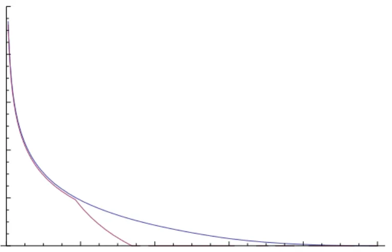
The following …gure illustrates the size of as a function ofk=k under our calibration, for values of = 0and = 0:28, where this last value is the average tari¤ in our sample of 71 developing countries. Notice that around k= 0:01k
we observe 0 2, so ignoring the gains for trade leads to an estimate of TFP
that is twice as high. Notice also that under = 0 the gains from trade fall smoothly with k, and still boost GDP over 10% for a relatively rich country with half the US capital-labor ratio. Meanwhile, under = 0:28 gains from trade suddenly fall abruptly for k > s(p ;0:28) 0:2 (as the economy ceases
9The bigger the di¤erence between the factor endowments between trading partners, the
Figure 1: as a function ofk=k for = 0 and = 0:28:
to be fully specialized) and 0:28 = 0 when k > x(p ;0:28) 0:33 (as the
economy ceases to trade.
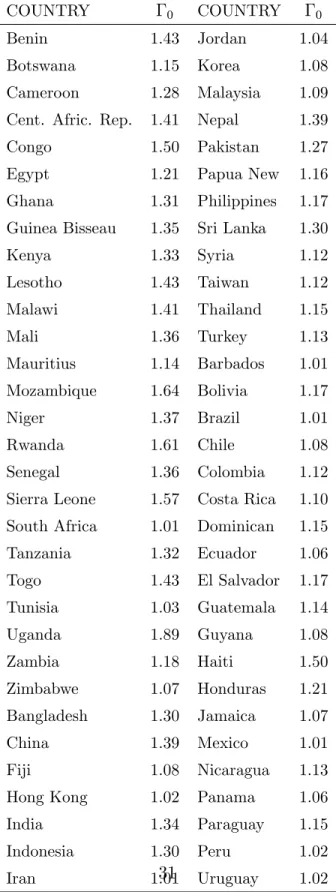
Just how big are the gains from trade in the world? The following table shows the potential gains under free trade, 0;for a representative sub-sample
of economies (the full sample appears in the Appendix). Table 1: Gains from openness
COUNTRY 0 COUNTRY 0
Bangladesh 1.30 Philippines 1.17 Brazil 1.01 Rwanda 1.61 China 1.39 South Africa 1.01 Haiti 1.49 Togo 1.43 India 1.34 Uganda 1.90 Malaysia 1.09 Zimbabwe 1.08
For the poorest nations, trade can almost double output (in the case of Uganda, the estimated increase in output under free trade is 89.8%), although
0 is less than 2% for a dozen countries in our sample which, like South Africa
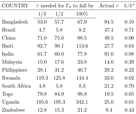
Of course, it does not take very high barriers to trade to make much of these gains to go away. For the same countries (again, …nd the rest in the Appendix), we list in the next table the levels of that make the gains from trade to be a third of 0, half of 0, or disappear altogether.
Table 2: Loss from barriers to trade
COUNTRY needed for 0 to fall by Actual k=k
1=3 1=2 100%
Bangladesh 53.0 57.7 67.9 94.5 0.10 Brazil 4.7 5.8 8.2 47.1 0.71 China 71.0 75.6 88.5 49.5 0.06 Haiti 92.7 98.1 113.6 27.7 0.04 India 61.7 66.0 77.8 91.0 0.08 Malaysia 15.0 17.6 23.8 14.0 0.39 Philippines 28.1 31.2 40.7 29.2 0.22 Rwanda 119.3 125.8 144.4 33.0 0.02 South Africa 4.8 5.8 8.3 21.2 0.70 Togo 79.8 84.9 98.8 19.5 0.05 Uganda 185.6 195.3 342.1 25.0 0.01 Zimbabwe 12.8 15.3 21.2 9.4 0.43
Clearly, many countries in the list have high tari¤s and waste most of the gains from trade. For instance, in the case of Bangladesh, the potential contribution to output from free trade would be a boost of 30%, and it would
take = 53% for a third of those gains to go away, and of = 68% to
wipe them out. The actual tari¤ rate of 94:5%, however, is enough to waste completely that boost in TFP. Similarly, Philippines is losing almost half its potential gains from trade because of restrictive commercial policy.
of doing trade, because they ignore transportation costs and many policy-induced non-tari¤ barriers. Recent direct measurement by Malherbe (2007) quanti…ed the cost of shipping cargo in and out of Rwanda, a landlocked country whose trucks have to go through Uganda and Kenya before reaching an international port in Mombassa. They found that the land-shipping alone cost about 80% of the value of exports. For imports this percentage is much higher (since containers come full inwards and half-empty outwards), and it has been quoted that bringing cargo into Kigali (Rwanda) from Mombassa can cost upwards of $6.500 per container. After adding the shipping cost to Mombassa, plus tari¤s, non-tari¤ barriers and the …nancial cost of nearly a month for the turnaround trip, the144% prohibitive rate that appears in the previous table does not seem farfetched.
In contrast, in countries such as Brazil and South Africa, in which k is relatively high, the tari¤ necessary to shut them from trade is very small. In fact, in both cases the observed tari¤ in 1985 is well above this level, so that they lost all the potential gains from trade.
Labor-abundant countries would specialize in producing only the labor-intensive good with low k < s(p; ). The country would acquire all the B it needs from the international market at a much lower opportunity cost, and hence the large gain from trade. In a less capital-poor country, wheres(p; )< k < x(p; );…rms still …nd it pro…table to produce more Athan needed by the local market, yet someB gets produced domestically as well. In this case, the potential gains are smaller as the countries endowment is not that di¤erent from the one of its trading partner (that is,k andk are close). Finally, a rich enough country, where k > x(p; ), will simply not trade. In that case, is bigger than the di¤erence between the international prices and the local prices that prevail without trade.
The next …gure shows the functions s(p; )=k and x(p; )=k as they vary with the tari¤ rate , for our calibration. One can verify that under free-trade, countries with less than54%of the US levels fork would be fully specialized in
Figure 2: s(p; )and x(p; ) as a function of
but their production would be diversi…ed. As increases, trade –and the gains it yields– fall. For example, if = 0:28, the average value of in our sample, the distortion towards allocating more resources in the B rather than
A industry is strong enough that only 28 countries in the sample remain fully specialized, and 14 don´t trade at all.
4.2
Productivity decomposition
We proceed now to make the decomposition. The usual approach yields
Y = bK L1
where b = . If an economy is in autarky, then = 1 = 1, and thus
Dividing by the number of workers, L, we get output per worker, or
Y
N = b
K L
L
N =
K
L h:
We use this expression in a otherwise standard level decomposition exercise, in which income di¤erence with respect to the US is measured as
Yi=Ni
YU S=NU S
= Ki
Li
=KU S LU S
(hi=hU S) i;
i U S
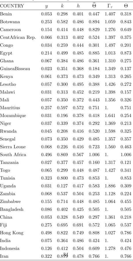
The two …rst components in the right hand side are standard in level de-composition exercises; …rst comes the e¤ect of di¤erent levels of capital per e¢ciency unit of labor, and then the amount of e¢ciency units of labor per worker. i.e., human capital. The product of the last two components is b, what usually appears for productivity, which we separate in in two parts: the productivity gain from trade and the TFP residual. The decomposition for our highlighted countries appears in the next table, and again the numbers for the full sample are in the Appendix.
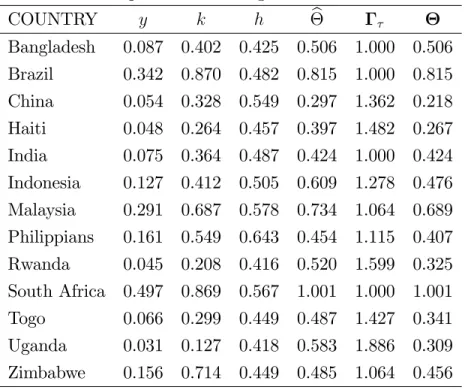
Table 3: Development accounting
COUNTRY y k h b
As expected, quite a few countries have 1, either because they are relatively high k and can expect little gains from trade (e.g., Brazil and Bar-bados), or because their tari¤s are so high that they waste most of those gains (e.g., Bangladesh and Pakistan). In this case b: On the other hand, for many countries happens to be very large, so even though some of the potential gains from trade are wasted due to protectionism, most are realized. For instance, in the usual decomposition, TFP in Rwanda is 52% of TFP in the U.S. However, once we take into account the gains from trade that such a poor country can enjoy (estimated as a boost of60% in output)– TFP is really much lower,32%. Other noteworthy cases are those of Congo, Haiti, Mozam-bique, Rwanda and Sierra Leone. In these countries is around or below 65% of c: On average, the trade-corrected TFP estimate in our sample is around 88% of b10.
Is there a way in which one can say that our estimated is a better num-ber than the usual b? In particular, is there any puzzling aspect of b as it is conventionally measured, that gets explained once we divide the trade and non-trade components of productivity? When we consider (by running a sim-ple OLS regression, for instance) the relationship between income per capita and standard closed-model TFP, b; we …nd high positive correlation, as ex-pected, but a large number of outliers countries for which TFP is either much higher or smaller than expected for its income level. Some examples would be Sierra Leone, Jordan, Uganda and Mozambique and Guatemala. However, for the case of the trade-corrected measure of TFP, ;this phenomena is less pronounced and the relationship between y and is much smoother. Hence, a large part of the relationship between y and b was due to international exchange, and once we correct for the gains from trade, estimated TFP falls. The R-squared of the regression of ony (both relative to the U.S.) is higher
10Note that in the case of b our results are not too distant from the literature. We redid
and, more importantly, the sum of squared residual is 43% smaller than that of the regression of b ony, and indication of a better …t.
4.3
TFP e¤ects of changes in terms of trade
Kehoe and Ruhl (2008) show that there is a strong link between the terms of trade and total factor productivity in the data of some countries (like the US and Mexico), and cite a number of other papers that have also pointed out this empirical fact.11 They also illustrate through a variety of macro models
that the standard approach cannot account for this relationship, which is a puzzle in need of an explanation. We believe that the model described in the previous sections provides one plausible mechanism to understand this puzzle: improvements in the terms of trade change the allocation of resources across sectors, inducing higher specialization in a way that increases productivity. To be precise, an increase in p induces a reallocation from KB to KA and from
LB to LA, and simultaneously raises b at the expense of a, in a manner that
is conducive to higher income and output. It is straightforward to see that as long as k < k then @Y
@p 0, as 1, 2 and 3 in (2) are increasing inp.
Furthermore, as Kehoe and Ruhl also argue, this …nding depends on how is output measured. Notice in particular that while in the model the sign of the e¤ect of terms of trade on real income is unambiguous, this is not necessarily the case if, for example, output is measured using a Laspeyres method and no PPP correction (as many countries do), especially when tari¤s are high. Measuring qA+B, using q =p=(1 + ), would be the equivalent to applying Laspeyres. After an increase inp, old prices (used in Laspeyres) put a premium onB overA, compared to new prices; similarly, domestic prices (which include the tari¤) put a premium on the imported good over the exported good. The real gains from trade may not be enough to compensate both biases. On the other hand, if one uses PPP corrected rather than domestic prices, these biases
11In the decade before the current …nancial crisis, several Latin American countries
do not exist, and the positive link between terms of trade and productivity is then unambiguous.12
How big is the e¤ect of changes in pon measured productivity? It depends on the level of income and the size of barriers to trade. In particular, recall from (4) that when the economy is poor enough to be specialized in the production of the labor intensive good –that is, whenk < s(p ; )– then is proportional top1
and thus the elasticity of b topis just given by1 = 0:57. In fact, the elasticity maintains that value even for a diversi…ed trading economy if = 0. In our sample of 71 countries, as in a large number of them k < s(p ; ), the median response of the gains from trade to a hypothetical change in the terms of trade displays that same elasticity. However, the e¤ects of p on b may be bigger or smaller if > 0; in our sample, the elasticity averages about 0:73, and is above 1:0 in10 cases.
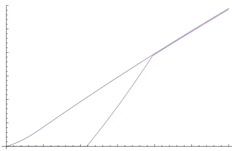
The e¤ect of p on b; for the case in which k = 0:375k ; is illustrated in the next …gure. It shows the variation in output when = 0 (the straight line above) and = 0:28 as functions of p, both as a proportion of the respective output leves at the original price. For the case of = 0; for instance, the straight line shows that when prices increase by 10%, output (i.e,F(K; Lj1:1
p; ) will be 5:7% above its original …gure (i.e,F(K; Ljp; ).
Whenk= 0:375and = 0:28, small variations ofpfromp are not enough to push the economy out of autarky. However, as p increases above certain level, it makes up for part of the negative impact of tari¤s on output. The economy starts to do some trade, and in the process the sectorial composition of output changes in favor of the good where the economy has comparative advantage, so productivity grows. Further increases in terms of trade allow the economy to produce increasingly more e¢cient sectorial mix, both on the
12Something similar happens when one considers the e¤ects of trade liberalization.
Figure 3: Change inF(K; L=p;0) and F(K; L=p;0:28) as pchanges.
…rst production stage (exporting more A and producing less B), and on the second (acquiring the utilized b at a smaller opportunity cost). Notice that in this interval the elasticity of output to p is larger than 0:57. For large enough variations inp(in this case above 41%) the economy specializes in the production of good A and hence the response of output to variations in p is the same as in the economy with no tari¤.
5
Conclusion
and countries. As opposed to Rodriguez-Clare (2006), which builds on Eaton and Kurtum(2002), there is no di¤usion in our model. Nonetheless, the model is able to capture some important features of the international commerce - poor countries do trade because of factor di¤erences - and so our measured gains from trade may be seen as a (large) lower bound of the gains from openness. As a matter of fact, they are close to those Rodriguez-Clare (2007) obtained in the pure trade model.
Moreover, the methodology we use does not capture the fact that barriers to trade do a¤ect investment decisions and so capital stocks, something we have shown in a previous paper (Ferreira and Trejos (2006)). In this sense, the current exercise is also limited as it takes stocks as given but does not consider that, if it were not for trade restrictions, they would be considerably larger.
Of course, the fact that poor countries with high tari¤s are still enjoying most of the gains from trade could be reverted if we have more realistic data, and not only nominal tari¤s data. Anderson and van Wincoop (2004) survey the literature on trade costs and show that for the OECD economies they are quite large and well above nominal tari¤s. We wanted, however, to use homogeneous data and the only source we know for this is the WorldBank database on nominal tari¤. A natural extension of this work is to use (and construct in some cases) data of trade cost based on gravitation models for a large set of economies.
References
[1] Acemoglu, D. and V. Guerrieri (2008) "Capital Deepening and Nonbal-anced Economic Growth,"Journal of Political Economy, vol. 116(3), 467-498.
[3] Anderson, J. and E. van Wincoop (2004), "Trade Costs",Journal of Eco-nomic Literature 42(3), 691-751.
[4] Barro, R. and J. W. Lee (2000), “International Data on Educational At-tainment: Updates and Implications,” NBER Working Paper No. 7911. [5] Caselli, F. (2005) "Accounting for Cross-Country Income Di¤erences," in:
Aghion, P. and Durlauf, S. (ed.), Handbook of Economic Growth, volume 1, chapter 9, Elsevier, 679-741.
[6] Cooley, T., Prescott, E., (1995), ”Economic Growth and Business Cycles.” in Cooley, T,Frontiers of Business Cycle Research, Princeton University Press.
[7] Corden, W. (1971), "The e¤ects of trade on the rate of growth", in Bhag-wati, Jones, Mundell and Vanek,Trade, Balance of Payments and Growth, (North-Holland), 117-143.
[8] Deardor¤, A. (2001), "Rich and Poor Countries in Neoclassical Trade and Growth," The Economic Journal, 111(April), 277-294.
[9] Easterly, R. Islam and J.E. Stiglitz (2001), "Shaken and stirred: Explain-ing growth volatility". In: B. Pleskovic and N. Stern, Editors, Annual World Bank Conference on Development Economics 2000, The World Bank , pp. 191–211.
[10] Eaton, J. and S. Kortum (2002), "Technology, Geography, and Trade,"
Econometrica 70(5), 1741-1780.
[11] Feenstra, R., Heston, A., Timmer, M. and H. Deng (2007), “Estimating Real Production and Expenditures across Nations: A Proposal for Im-proving the Penn World Tables". World Bank Policy Research Working Paper #4166.
Produc-tivity" The B.E. Journal of Macroeconomics, Vol. 8 : Iss. 1 (Topics), Article 3.
[13] Ferreira, P. C. and A. Trejos (2006), “On the Long-run E¤ects of Barriers to Trade,”International Economic Review, 47(4), 1319-1340.
[14] Hall,R. and C. Jones (1999), “Why Do Some Countries Produce So Much More Output per Worker Than Others?,” Quarterly Journal of Eco-nomics, 114(1): 83-116.
[15] Hsieh, C. and P. Klenow (2007), "Misallocation and Manufacturing TFP in China and India," NBER Working Papers No. 13290.
[16] Kehoe, P. J. and T. J. Kehoe. (1994) “Capturing NAFTA’s Impact With Applied General Equilibrium Models,”FRB Minneapolis - Quarterly Re-view, 18(2), 17-34.
[17] Kehoe, T. and K. Ruhl (2008), ”Are Shocks to the Terms of Trade Shocks to Productivity?,” Review of Economic Dynamics, vol. 11(4), 707-720. [18] Kehoe, T. and K. Ruhl (2006), “Sudden Stops, Sectorial Reallocations,
and Real Exchange Rates,” University of Minnesota and University of Texas at Austin.
[19] Klenow, P. J. and A. Rodriguez-Clare (1997), “The Neoclassical Revival in Growth Economics: Has it Gone Too Far?,” in Ben S. Bernanke and Julio J. Rotemberg, eds, NBER Macroeconomics Annual 1997 (Cambridge, MA: The MIT Press), 73-103.
[20] Malherbe, S. (2007), "A Diagnostic Analysis of the Kigali-Mombassa Transport Corridor", Genesis, South Africa.
[22] Mendoza, E. G. (2006), “Endogenous Sudden Stops in a Business Cycle Model with Collateral Constraints: a Fisherian De‡ation of Tobin’s Q,” manuscript, University of Maryland.
[23] Meza, F and E. Quintin (2007), “Financial Crises and Total Factor Pro-ductivity,” The B.E. Journal of Macroeconomics, 7:1 (Advances), article 33.
[24] Prescott, E. (1998), “Needed: a Total Factor Productivity Theory,” In-ternational Economic Review, 39(3): 525-552.
[25] Psacharopoulos, G. (1994), “Returns to Investment in Education: A Global Update,” World Development, 22(9): 1325-1343.
[26] Restuccia, D. and R. Rogerson, (2008), "Policy Distortions and Aggregate Productivity with Heterogeneous Plants," Review of Economic Dynamics, vol. 11(4), 707-720.
[27] Rodriguez-Clare, A. (2007), "Trade, Di¤usion and the Gains from Open-ness," NBER Working Paper No. 13662.
[28] Rodriguez-Clare, A., Trejos, A. and M. Sáenz (2003), "Comprendiendo el crecimiento de 50 aneos en Costa Rica," Manuel Agosín y Andrés Solimano (eds), InterAmerican Development Bank Press.
[29] Summers, R. and A. Heston (1991) "The Penn World Table (Mark 5): An Expanded Set of International Comparisons, 1950-1988," The Quarterly Journal of Economics, vol. 106(2), 327-68..
[30] Trejos, A. (1992), “On the Short-Run Dynamic E¤ects of Comparative Advantage Trade,” University of Pennsylvania.
[31] Ventura, J. (1997), “Growth and Interdependence”,Quarterly Journal of Economics, 112(1): 57-84
A
Appendix
We present in details the derivation of the production function used in the paper. The pro…t maximization problems in the de…nition of stationary equi-librium yield:
(1 a)
a
kA =
(1 b)
b
kB (5)
q(1 a)kAa = (1 b)kBb
b
(1 ) = qa;
Similarly, the market clearing conditions forK andLcan be transformed into:
kA+ (1 )kB =k;
where =LA=Land the production functions are then written as
A = Lk a
A andB = (1 )Lk
b
B:
In the case of an economy that do not trade the conditionpa+b=pA+B
is substituted instead for the conditionsa=A; b=B. In that case, the above solves into
= (1 a)
1 ;
where = a+ (1 ) b: Then, more algebra yields the solutions:
kA= a
(1 a)
1
k and kB = b
(1 b)
1
k:
These imply that total output Y (undera =A; b =B) is:
Y = 4K L
1
where
4 =
(1 )1
[ a
a (1 a)
1 a
] [ b
b (1 b)
1 b
]1
(1 )1 :
From 5 and the expression of q one can derive:
x= 1 " p 1 + a
a (1 a)
1 a
b
b (1 b)
1 b
# 1
b a
where x is the minimal capital level for the economy not to trade (i.e,x( ; p)
in (2)). Likewise, following similar steps one can derive:
s1 =
" p 1 + a b b 1 a 1 b
1 b#
1 b a
(7)
s2 =
" p 1 + a b a 1 a 1 b
1 a#
1 b a
;
where s1 corresponds to s( ; p) in (2)
In the case that the economy is diversi…ed and export A and import B, the solution of the factor allocation problem is:
LA= ss22L Ks1 LB = K ss2 s11L
KA=s1ss2L K
2 s1 KB =s2
K s1L
s2 s1
: (8)
From the expression above and (7) the equilibrium expression of Y in this case is:
where:
2 = (1 )
1
p (1 + )
1 +
s b
2 ps
a
1
s2 s1
(10)
3 = (1 )
1
p (1 + )
1 +
ps a
1 s2 s
b
2 s1
s2 s1
Finally, when the economy is fully specialized in A (so that k < s1), one
can derive (after imposingKB =LB=B = 0)from (5), (8) and the expression
for the equilibrium in the market for intermediate goods:
Y = 1K
a
L1 a
; (11)
where:
1 = (1 )
1
p1 (1 + )
Table A.1: Gains from openness
COUNTRY 0 COUNTRY 0
Table A.2: Loss from barriers to trade
COUNTRY needed for 0 to fall by Actual k=k
1=3 1=2 100%
Table A.2 (cont.): Loss from barriers to trade
COUNTRY needed for 0 to fall by Actual k=k
1=3 1=2 100%
Table 3: Development accounting
COUNTRY y k h b
Table 3 (cont.): Development accounting COUNTRY y k h b