MEASURING DRIVERS’ EFFECT IN A COST MODEL BY MEANS OF ANALYSIS OF VARIANCE

ISSN: 1546-9239

©2013 Science Publication

doi:10.3844/ajassp.2013.1570.1574 Published Online 10 (12) 2013 (http://www.thescipub.com/ajas.toc)

MEASURING DRIVERS’ EFFECT IN A COST

MODEL BY MEANS OF ANALYSIS OF VARIANCE

Maria Elena Nenni

Department of Industrial Engineering, University of Naples “Federico II”, Naples, Italy

Received 2013-09-17, Revised 2013-09-27; Accepted 2013-10-24

ABSTRACT

In this study the author goes through with the analysis of a cost model developed for Integrated Logistic Support (ILS) activities. By means of ANOVA the evaluation of impact and interaction among cost drivers is done. The predominant importance of organizational factors compared to technical ones is definitely demonstrated. Moreover the paper provides researcher and practitioners with useful information to improve the cost model as well as for budgeting and financial planning of ILS activities.

Keywords: Logistic Support, Maintenance, Cost Model, Lifecycle Management, ANOVA

1. INTRODUCTION

A cost model is a mathematical algorithm or parametric equation that converts input data into the cost of a product, service or project. The result is widespread used in economic evaluation to obtain approval to proceed and is factored into business plans, budgets and other financial planning. A cost model most often involves synthesizing data from a number of sources and a persistent methodological problem is how to deal with the input uncertainty. Many authors use a Monte Carlo method (You et al., 2009; Yang, 2011; Loizou and French, 2012) to propagate the uncertainty from the input data to the result variables. The goal is to obtain unbiased estimates of the central tendencies (mean or median) or some other representations of the distribution of the cost. Even better is the ANOVA method that allows partitioning of observed variance into components attributable to different source of variation (Ellis, 2010). In a cost model are usually identified various relevant factors and ANOVA is used to select the factors that are significantly influent on the model (Charongrattanasakul and Pongpullponsak, 2011; Al-Hazza et al., 2011).

This study aims to complete the analysis of a specific cost model firstly proposed by the author and then evaluated through the Monte Carlo method (Nenni, 2013a).

The cost model has been developed in the field of the Integrated Logistic Support (ILS). ILS refers to activities implemented by a Contractor Logistic Support (CLS) in a continuous way to ensure the best system capability at the lowest possible life cycle cost (ILS, 2012).

2. THE COST MODEL

The CLS needs of cost estimates to develop annual budget requests, to evaluate resource requirements at key decision points and to choose about investment. Nenni (2013a) has developed on the basis of ILS (2012) a specific cost model, really fitting with the ILS issues.

The model use technical parameters provided through a RAM analysis: Mean Time Between Failures (MTBF), Mean Time To Restore the System (MTTRS), Mean Time Between Preventive maintenance (MTBP) and Mean Time To Preventive maintenance (MTTP).

Additional parameters are then related to the organizational issues. Basically, we take into consideration a Skill Factor (SF≥1), decreasing down to the asymptotic value of 1 as experience, training and expertise owned by ILS staff grow. The SF has impact on the time to restore the system. The Delay Time is introduced to analyze specifically the reason because an activity could be delayed. It is split up in Logistic Delay Time (DTL), in Staff Delay Time (DTS) and in Spare parts Delay Time (DTSp). The last one is a well-known parameter because it affects many actors in every supply chain. It takes into consideration the time-wasted because the spare part is not available in stock or the supplier provides it in delay. DTS describes instead the time-wasted because the staff is not well organized to do the activities in an efficient way. Finally DTL catches the time-wasted for any logistic reason, lack of informations, fault diagnosis. ILS performance indicators are Mean Time Between Maintenance (MTBM), Mean Down Time (MDT) and operational Availability (Ao). Accordingly with main reference (ILS, 2012) they are calculated as follow in Equation 1-3:

1 MTBM

1 1

MTBF MTBP

=

+ (1)

(

)

SF MTTRS DT DT DT _MTTP

MTBF MTBP

MDT

1 1

MTBF MTBP

⋅ + + +

+ =

+

(2)

MTBM Ao

MTBM MDT

=

+ (3)

The annual ILS cost (Nenni, 2013b) is split up in cost for Preventive Maintenance (PM) and cost for Corrective Maintenance (CM) as in Equation 4-5:

(

)

(

)

PM Sh SP

OT

C c n MTTP c

MTBP

= ⋅ ⋅ + ⋅ (4)

where, cSh is the average hourly cost for an employee, n

is the number of people in staff, cSP is the average cost

for spare parts and material and the Operating Time (OT) is the period during a system works.

Similarly the annual cost for corrective maintenance is:

(

)

(

)

CM Sh

OT

C = k c n MTTRS + c

MTBF

⋅ ⋅ ⋅ ⋅ (5)

where, k>1 increases the cost in order to take into account several complications that often occur with a breakdown.

An additional cost category in the model is related to the penalty Cost for Poor performance (CP) that is based on the ILS indicators and calculated as shown in the Table 1. The introduction of a penalty cost allows us to consider the trade-off between costs and performance in accordance with recommendations by Asjad et al. (2013).

The MTBM should be in an optimal range [MTBM1,

MTBM2] to avoid the system stops too frequently and a

little use of preventive maintenance both. The MDT exceeding its target reveals a problem of maintainability. Finally penalty cost related to AO is a continuous

function at times as in Table 1, where x2 > x1 and both are < 1 and P’’A>P’A.

The last cost element in the model concerns the Delay Time (Equation 6). We don’t consider cost incurred directly because an activity is delayed. In fact it is just included in penalty cost through the MDT indicator. CDT links Delay Times to the investment in

their improvement or to maintain them constant as follow:

0

DT

DT C =γ ln

DT

 

⋅  

  (6)

Table 1. From level 2 to level 3 of maturity (Scor)

Indicators Target Penalty cost (CP)

MTBM ≤ MTBM1 PMTBM

MTBM ≥ MTBM2 P’MTBM

MDT ≥ MDTT PMDT

Ao ≤ AT PA

Ao ≤ x1·AT P’A

Ao ≤ x2·AT P’’A

Table 2. Cost drivers used for sensitivity analysis

Cost drivers Type of parameter

MTBF Technical

MTTRS Technical

MTBP Technical

MTTP Technical

DTL Organizational

DTS Organizational

DTSp Organizational

cSh Organizational

cSp Organizational

SF Organizational

DT is the expected value for the current year and γ is a constant calculated on the basis of a relationship between investment and DT that could be known.

Now the annual cost function (CILS) can be

formulated as in Equation 7:

L S Sp

ILS PM CM P DT DT DT

C = C + C + C + C + C + C (7)

From the general model it is possible to extrapolate drivers or factors that may have an impact on the performance. A preliminary list of these drivers is presented in the Table 2.

In the previous work the author has just calculated the relative importance of each driver on the annual ILS cost through a sensitivity analysis and she has concluded that the organizational-logistic parameters are the most influencing and critical. In this case CLS should pay a lot of attention in all the aspects of managing ILS activities. Technical parameters as MTBF and MTTRS have a poor impact. So in this study attention has been focused on the analysis of the organizational parameters as in Table 2. The knowledge of the contribution of individual factors is a key for every decision process. Analysis of Variance (ANOVA) is a method of portioning variability into identifiable sources of variation and the associated degree of freedom in an experiment.

3. THE ANOVA PROCEDURE

In general, the purpose of Analysis of Variance (ANOVA) is to test for analyzing the effect of categorical factors on a response.

Table 3. Drivers and their level

Cost drivers Level 2 Level 1

DTL 0,4 0,8

DTS 0,5 0,9

DTSp 0,3 1

SF 1 2

Table 4. Experimental design using L8 orthogonal array

Expt. n° DTL DTS DTSP SF

1 2 1 2 2

2 2 2 1 1

3 2 1 2 1

4 1 2 1 1

5 1 2 1 2

6 1 2 2 2

7 2 1 1 1

8 1 1 2 2

An ANOVA decomposes the variability in the response variable amongst the different factors, in order to determine: (i) which factors have a significant effect on the response (ii) how much of the variability in the response variable is attributable to each factor.

A factorial design is used to evaluate all the factors simultaneously. The treatments are thus combinations of levels of the factors. We have considered two levels for each factor (Table 3): (i) high performance (2) (ii) low performance (1).

Through the Taguchi Orthogonal Array (Hinkelmann, 2012), we have considered a selected subset of combinations of multiple factors at multiple levels.

Taguchi method based design of experiments has been used to study effect of four cost drivers on the response factors. For selecting appropriate orthogonal arrays, degree of freedom of array is calculated and a Taguchi based L8 orthogonal array is selected. Accordingly, 8 experiments were carried out to study the effect of drivers (Table 4). Each experiment was repeated six times in order to reduce experimental error.

L8 orthogonal array has (8*6-1) = 47 Degree of Freedom (DOF), in which 4 were assigned to four factors (each one 1 DOF) and 43 DOF was assigned to the residual. The response factors are the ILS annual cost (CILS) and

the operational Availability (Ao). In Table 5 and 6 are reported ANOVA summary data for each response factor.

4. RESULTS AND ANALYSIS OF

EXPERIMENTS

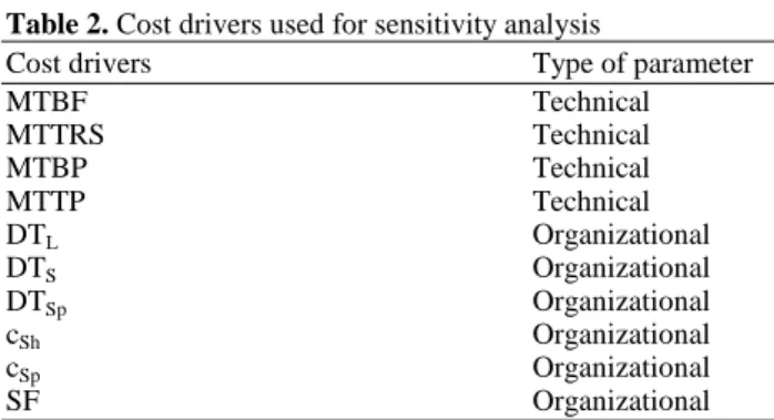
Table 5. ANOVA summary data for CILS data

Factor DOF SS MS F Flim. P%

DTL 1 12121415,60 12121415,6 12,61404807 0,004 13

DTS 1 9384647,108 9384647,108 9,766053208 0,004 10

DTSp 1 28015541,59 28015541,59 29,15413511 0,004 31

SF 1 229221,4947 229221,4947 0,238537399 0,004 0

Res. 43 41320666,30 960945,7279 45

Tot. 47 91071492,09 1937691,321 2,016441996 100

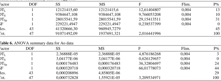
Table 6. ANOVA summary data for Ao data

Factor DOF SS MS F Flim. P%

DTL 1 2,36888E-05 2,36888E-05 4,876186268 0,004 3

DTS 1 3,04177E-06 3,04177E-06 0,626129657 0,004 0

DTSp 1 0,000176483 0,000176483 36,32804697 0,004 24

SF 1 0,000320718 0,000320718 66,01778073 0,004 44

Res. 43 0,000208896 4,85805E-06 29

Tot. 47 0,000732828 1,55921E-05 3,209534971 100

In the analysis, the F-ratio is a ratio of the mean square error to the residual error and is traditionally used to determine the significance of a factor. Table 5 and 6 show the result of Fisher analysis that was carried out for a level of significant of 5%, i.e., for 95% a level of confidence. We have then a Flim.(0,05; 1; 43) = 0,004

(see the F distribution table in Montgomery, 2010). Since the test statistic is much larger than the critical value for all the factors, we reject the null hypothesis of equal population means and conclude that there is a (statistically) significant difference among the population means. The overall test F is significant, indicating that the model as a whole accounts for a significant portion of the variability in the dependent variable.

The last column of the tables shows the percent contribution (P) of each factor as the total variation, indicating its influence on the result. The percentage contribution P can be calculated as in Equation 8:

factor total

SS P =

SS (8)

where, SS is the sum of the squared deviations. It is illustrated that DTSp has the most significant effect on the

output response CILS. Other significant parameters are, in

turn, DTL and DTS. For the response factor Ao, the most

significant factor is the SF followed again by DTSp.

5. CONCLUSION

This study has discussed an application of the ANOVA and Taguchi method for investigating the effects of cost drivers on the cost model for the ILS activities. The factors were selected taking into consideration results from a previous work of the author.

From the analysis of the results using the ANOVA and Taguchi’s optimization method, the following can be concluded from the present study:

• The significance of organizational parameters rather than technical parameters has been confirmed • DTSP results a very impacting factor both on CILS and

Ao and it supports in a quantitative way the interest in the ILS field for the integration among supply chain factors (Nenni and Giustiniano, 2013)

• SF impacts highly on Ao but absolutely not on CILS. It is probably due to the model structure in

which the average hourly cost for an employee (cSh) is not split up for different level of skill.

Then in the model it is considered the same cost of an employee not depending from his level of skill. This point should be better developed

6. REFERENCES

Al-Hazza, M.H.F., E.Y.T. Adesta, A.M. Ali, D. Agusman and M.Y. Suprianto, 2011. Energy cost modeling for high speed hard turning. J. Applied

Sci., 11: 2578-2584. DOI:

10.3923/jas.2011.2578.2584

Asjad, M., S.K. Makarand and O.P. Gandhi, 2013. A life cycle cost based approach of O&M support for mechanical systems. Int. J. Syst. Assurance Eng. Manage., 4: 1-14.DOI: 10.1007/s13198-013-0156-7 Charongrattanasakul, P. and A. Pongpullponsak, 2011.

Choi, J., 2009. O&S cost growth. Proceedings of the 3rd Annual Navy/Marine Corps Cost Analysis Symposium, Quantico, (SQ’ 09), Gray Research Center, VA.

Ellis, P.D., 2010. The Essential Guide to Effect Sizes: Statistical Power, Meta-Analysis and the Interpretation of Research Results. 1st Edn., Cambridge University Press, Cambridge, ISBN-10: 0521142466, pp:173.

Hellstrom, M., I. Ruuska, K. Wikstrom and D. Jafs, 2013. Project governance and path creation in the early stages of finnish nuclear power projects. Int. J. Project Manage., 31: 712-723. DOI: 10.1016/j.ijproman.2013.01.005

Hinkelmann, K., 2012. Design and Analysis of Experiments, Special Designs and Applications. 1st Edn., John Wiley and Sons, Hoboken, N.J., ISBN-10: 0470530685, pp:600.

ILS, 2012. Integrated Logistics Support. Army Regulation 700-127, Department of the Army, Washington, USA.

Loizou, P. and N. French, 2012. Risk and uncertainty in development: A critical evaluation of using the Monte Carlo simulation method as a decision tool in real estate development projects. J. Property Investment Finance, 30: 198-210. DOI: 10.1108/14635781211206922

Montgomery, D.C., 2010. Design and Analysis of Experiments, Minitab Manual. 7th Edn., John Wiley and Sons,Hoboken, NJ.,ISBN-10: 0470169907, pp: 114.

Nenni, M.E. and L. Giustiniano, 2013. Increasing integration across the supply chain through an approach to match performance and risk. Am. J. Applied Sci., 10: 1009-1009. DOI: 10.3844/ajassp.2013.1009.1017

Nenni, M.E., 2013a. Cost assessment for Integrated Logistic Support (ILS) activities. Int. J. Indus. Eng. Theory Appli. Pract.

Nenni, M.E., 2013b. A cost model for integrated logistic support activities. Adv. Operat. Res., 2013: 6-6. DOI: 10.1155/2013/127497

Yang, J., 2011. Convergence and uncertainty analyses in Monte-Carlo based sensitivity analysis. Environ. Modell. Software, 26: 444-457. DOI: 10.1016/j.envsoft.2010.10.007