Application of CFD code for simulation of an inclined snow chute flow

Vol. 3, Issue 2, March -April 2013, pp.1309-1319

Application of CFD code for simulation of an inclined snow chute

flow

R K Aggarwal* and Amod Kumar

Snow and Avalanche Study Establishment, Research and Development Centre,

HIM PARISAR, Sector 37-A, Chandigarh *E-mail:rakeshaditya11@rediffmail.com

Abstract

In this paper, 2-D simulation of a 61 m long inclined snow chute flow and its interaction with a catch dam type obstacle has been carried out at Dhundhi field research station near Manali, Himachal Pradesh (India) using a

commercially available computational fluid

dynamics (CFD) code ANSYS Fluent. Eulerian non-granular multiphase model was chosen to model the snow flow in the surrounding atmospheric air domain. Both air and snow were assumed as laminar and incompressible fluids. User defined functions(UDF) were written for the computation of bi-viscous Bingham fluid viscosity and wall shear stress of snow to account for the slip at the interface between the flowing snow and the stationary snow chute surface. Using the proposed CFD model, the velocity, dynamic pressure and debris deposition were simulated for flowing snow mass in the chute. Experiments were performed on the snow chute to validate the simulated results. On comparison, the simulated results were found in good agreement with the experimental results.

Keywords:

1. Introduction

Avalanche dynamics numerical models are useful tools for avalanche hazard mapping to assess risk to different infrastructure on account of snow avalanches. Several models are available for describing the dynamics of snow avalanches. Some of the popular avalanche dynamics models are Voellmy [1], Perla et al. [2] and Christen et al. [3]. These models describe the avalanche as a solid block of snow, deformable body, in particular as a continuum, with the hydraulics approach based on depth-averaged equations or as a granular material. These models are used in a number of Countries and can predict the run-out distance and flow velocity of a snow avalanche in 2-D and 3-D terrains. The computational requirements of these models are quite low. However, it is not possible to use these models to determine the vertical velocity distribution and pressure as these are based on depth-averaged equations. There are also some other models which are based on a different numerical framework. Lang

et al. [4, 5, 6] proposed the AVALNCH model which is based on the numerical solution of Navier- Stokes (N-S) equations. Recent work by Bovet et al. [7] and ODA et al. [8] use CFD techniques solving N-S equations for avalanche flow. Different approaches are also used to describe the constitutive behavior of flowing snow: Newtonian fluids, Criminale-Ericksen-Filby fluid [9], Bingham fluid [10, 11, 12], Nishimura et al. [13] or Cross fluid [14]. It is observed that snow avalanche flows down the mountain just like a fluid and it comes to complete rest in the run-out zone (slope angle < 120) and piles up to form debris [10]. This debris presents the solid behavior of snow. By the basic property of a Newtonian fluid, it keeps on deforming till some stress is acting on it. So, if flowing snow is modeled as a Newtonian fluid, snow will keep on moving till it completely spreads over the ground and flow depth reaches to zero. This is contrary behavior in comparison to the observed one where snow is seen to come to rest with a finite depth where stress is non-zero. That means for the snow, a yield value occurs when the deformations become small, and consequently the snow can rest with a non-zero shear stress.

Vol. 3, Issue 2, March -April 2013, pp.1309-1319

Figure 1. View of snow chute setup at Dhundhi (20 km from Manali, H. P., India)

much has been described about the application of these models for computation of wall slip, snow debris and run-out distance for snow chute and real avalanche flows. Another goal of the present paper is to demonstrate the capability of user friendly commercial CFD code for modeling of complex snow flow under gravity.

2. Methodology

2. 1. About the experimental site

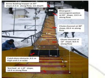
The experimental work was carried out on the 61 m long and 2 m wide snow chute at the Dhundhi station. At this site, on an average, cumulative seasonal snowfall is approximately 11m and winter ambient temperatures vary from a minimum of -150 C to maximum of +100 C. The chute consists of five sections as shown in Fig. 1. The bottom surface of the chute is made of mild steel (MS) sheets. The side railing of the snow chute is 1 m high which is covered with transparent polycarbonate sheets to minimize friction between the side walls and the flowing snow. The transparent side walls also facilitate observation of the flow through the side walls of the chute. Alternate red and yellow colors are painted at every 0.5 m interval on the bottom surface of the chute for ease in measurement of snow flow parameters. The snow chute structure is erected on the concrete pillars. There is provision for changing angle of tilt of 5.5 m long snow hopper from 300 to 450 with the help of hydraulic system. In the present studies, this angle is kept fixed at 350. Snow hopper can be fed maximum up to 11.0 m3 volume of snow. The 13.5 m long diverging-converging channel inclined at 350 is provided to ensure that snow does not move like a solid block down the chute and proper fluidization of snow takes place. The 22 m long chute channel inclined at 300 acts as accelerating path for the snow and snow attains maximum velocity near the end of this channel. The 8 m long

chute channel inclined at 120 ensures reduction in momentum of snow flow and snow completely comes to a halt on the 12 m test bed inclined at an angle of -1.80.

2.2. Mathematical model

In ANSYS Fluent software, three different Euler-Euler multiphase models are available: the volume of fluid (VOF) model, the mixture model, and the Eulerian model. In the present work, non-granular immiscible Eulerian fluid model (fluid-fluid flows) was chosen for solving a set of momentum and continuity equations for incompressible snow and air phases. Coupling is achieved through the pressure and interphase exchange coefficients. The immiscible fluid model for Eulerian multiphase enables sharp interface treatment between the phases [16].

2.2.1. Flow governing equations [16]

The description of multiphase flow incorporates the concept of phasic volume fractions, denoted here by αq. Volume fractions

represent the space occupied by each phase, and the laws of conservation of mass and momentum are satisfied by each phase individually. Air is considered primary phase p and snow as secondary phase q. The basic flow governing equations solved by ANSYS Fluent are described below.

The volume of phase q, is defined as:

So, the effective density of phase q is αqρq where

ρq is the density (kg m-3) of the phase q in the

solution domain. V' is the total volume. 2.2.1.1. Continuity equation

Vol. 3, Issue 2, March -April 2013, pp.1309-1319

The solution of (3) for the snow phase along with the condition that the volume fractions sum to one allows for the calculation of the volume fraction of the air. is the velocity vector of snow. 2.2.1.2. Fluid-fluid momentum equations

The conservation of momentum for a fluid phase q is:

+ + (4) is the phase stress-strain tensor of phase q, given as:

q and λq are shear and bulk viscosity of

phase q, respectively. is the unit tensor. Since snow is considered incompressible, second term in (5) vanishes. is acceleration due to gravity (m s-2) and p' is the hydrodynamic pressure shared by both the primary and secondary phase (Pa). Kqp is the

interphase momentum exchange coefficient (kg m-3 s-1). In the present work, it is calculated as below:

Where f is the drag function which can be given by model of Schiller and Naumann as:

CD is the drag coefficient which is function of

relative Reynolds number Re, given as:

For symmetric model, density ρqp (kg m-3) is

calculated from volume averaged properties:

Particulate relaxation time is given as :

Where viscosity is calculated as:

Here, droplet diameter dqp=0.5*(dp+dq).

For single dispersed phase, dp=dq. So, dqp= dq is the

diameter of the secondary dispersed phase set at default value of 10-5 m for all the simulations. As inter granular collisions, cohesions and other significant granular properties of snow are neglected in the present model, the flow rheology

of snow is similar to a continuum fluid. Momentum equation for the primary phase p is written similar to (4).

2.2.2. Snow as non-Newtonian fluid

The constitutive equation of a Bingham fluid is made up of two parts. First, if the shear stress intensity τ (N m-2) is below a yield stress value τ0

(N m-2), no deformation takes place and material behaves as a rigid solid. Second, if the stress intensity is above this value, deformation takes place and is proportional to the amount that the stress level exceeds τ0 (Fig. 2).

Figure 2. Flow rheology of a bi-viscous Bingham fluid

Following the work of Dent et al. [10], in this paper, bi-viscous Bingham fluid model has been used which allows small deformations to take place according to a linear viscous flow law in the locked portion of the flow (dotted lines inFig. 2). The viscosity used in this region (in the present paper taken as 104 Pa s) is taken so high that the resulting deformation can be neglected relative to deformations outside this region [8]. Adopting from [8, 10, 17, 18], the effective Newtonian viscosity for a Bingham fluid can be given as:

Where k= viscosity coefficient of snow after the yield region (Pa s). Following [8], we have taken value of k as 0.02 Pa s for all the simulations. This value is reasonable as snow flows like a Newtonian fluid with low viscosity after the yield region. strain rate in the locked flow regime(s

-1

). This is computed as:

The yield strength of snow τ0 is considered

as the function of hydrodynamic pressure p', cohesion strength c and internal friction angle of snow φ[8, 19]:

Substituting (15) into (13), can be re-written as:

Vol. 3, Issue 2, March -April 2013, pp.1309-1319

which is related to the second invariant of rate of deformation tensor, as [16]:

Here

On simplification and algebraic manipulation, (17) reduces to

u, v are the velocities in X & Y-direction, respectively.

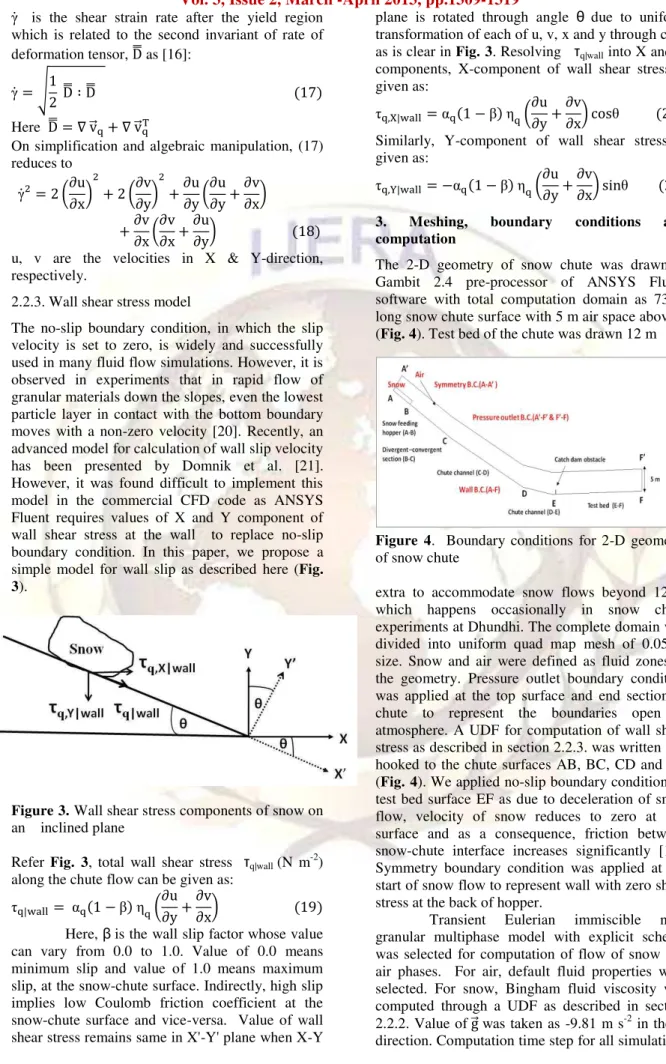
2.2.3. Wall shear stress model

The no-slip boundary condition, in which the slip velocity is set to zero, is widely and successfully used in many fluid flow simulations. However, it is observed in experiments that in rapid flow of granular materials down the slopes, even the lowest particle layer in contact with the bottom boundary moves with a non-zero velocity [20]. Recently, an advanced model for calculation of wall slip velocity has been presented by Domnik et al. [21]. However, it was found difficult to implement this model in the commercial CFD code as ANSYS Fluent requires values of X and Y component of wall shear stress at the wall to replace no-slip boundary condition. In this paper, we propose a simple model for wall slip as described here (Fig. 3).

Figure 3. Wall shear stress components of snow on an inclined plane

Refer Fig. 3, total wall shear stress τq|wall (N m-2)

along the chute flow can be given as:

Here, βis the wall slip factor whose value can vary from 0.0 to 1.0. Value of 0.0 means minimum slip and value of 1.0 means maximum slip, at the snow-chute surface. Indirectly, high slip implies low Coulomb friction coefficient at the snow-chute surface and vice-versa. Value of wall shear stress remains same in X'-Y' plane when X-Y

plane is rotated through angle due to uniform transformation of each of u, v, x and y through cos as is clear in Fig. 3. Resolving τq|wall into X and Y

components, X-component of wall shear stress is given as:

Similarly, Y-component of wall shear stress is given as:

3. Meshing, boundary conditions and

computation

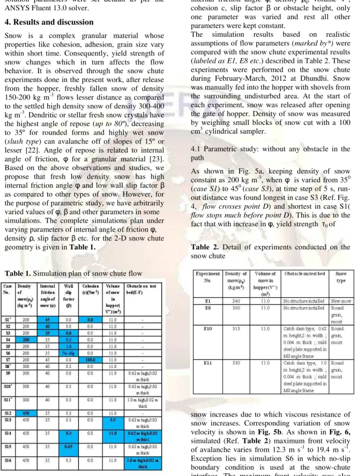
The 2-D geometry of snow chute was drawn in Gambit 2.4 pre-processor of ANSYS Fluent software with total computation domain as 73 m long snow chute surface with 5 m air space above it (Fig. 4). Test bed of the chute was drawn 12 m

Figure 4. Boundary conditions for 2-D geometry of snow chute

extra to accommodate snow flows beyond 12 m which happens occasionally in snow chute experiments at Dhundhi. The complete domain was divided into uniform quad map mesh of 0.05 m size. Snow and air were defined as fluid zones in the geometry. Pressure outlet boundary condition was applied at the top surface and end section of chute to represent the boundaries open to atmosphere. A UDF for computation of wall shear stress as described in section 2.2.3. was written and hooked to the chute surfaces AB, BC, CD and DE (Fig. 4). We applied no-slip boundary condition on test bed surface EF as due to deceleration of snow flow, velocity of snow reduces to zero at this surface and as a consequence, friction between snow-chute interface increases significantly [13]. Symmetry boundary condition was applied at the start of snow flow to represent wall with zero shear stress at the back of hopper.

Vol. 3, Issue 2, March -April 2013, pp.1309-1319

solution parameters were set default as per the ANSYS Fluent 13.0 solver.

4. Results and discussion

Snow is a complex granular material whose properties like cohesion, adhesion, grain size vary within short time. Consequently, yield strength of snow changes which in turn affects the flow behavior. It is observed through the snow chute experiments done in the present work, after release from the hopper, freshly fallen snow of density 150-200 kg m-3 flows lesser distance as compared to the settled high density snow of density 300-400 kg m-3. Dendritic or stellar fresh snow crystals have the highest angle of repose (up to 80º), decreasing to 35º for rounded forms and highly wet snow (slush type) can avalanche off of slopes of 15º or lesser [22]. Angle of repose is related to internal angle of friction, φ for a granular material [23]. Based on the above observations and studies, we propose that fresh low density snow has high internal friction angle φ and low wall slip factor β as compared to other types of snow. However, for the purpose of parametric study, we have arbitrarily varied values of φ, βand other parameters in some simulations. The complete simulations plan under varying parameters of internal angle of friction φ,

In a particular comparison out of parameters; internal friction angle φ, density ρq, volume V'',

cohesion c, slip factor β or obstacle height, only one parameter was varied and rest all other parameters were kept constant.

The simulation results based on realistic assumptions of flow parameters (marked by*) were compared with the snow chute experimental results (labeled as E1, E8 etc.) described in Table 2. These experiments were performed on the snow chute during February-March, 2012 at Dhundhi. Snow was manually fed into the hopper with shovels from the surrounding undisturbed area. At the start of each experiment, snow was released after opening the gate of hopper. Density of snow was measured by weighing small blocks of snow cut with a 100 cm3 cylindrical sampler.

4.1 Parametric study: without any obstacle in the path

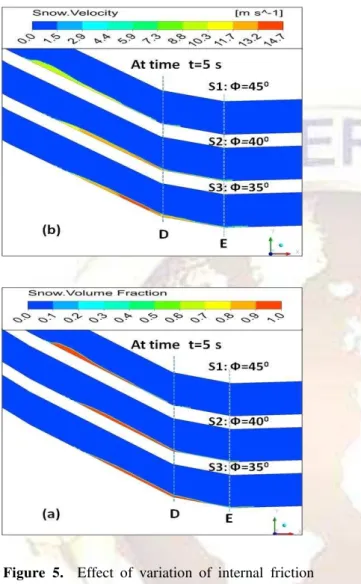
As shown in Fig. 5a, keeping density of snow constant as 200 kg m-3, when φ is varied from 350 (case S1) to 450 (case S3), at time step of 5 s, run-out distance was found longest in case S3 (Ref. Fig. 4, flow crosses point D) and shortest in case S1( flow stops much before point D). This is due to the fact that with increase in φ, yield strength τ0 of

density ρ, slip factor β etc. for the 2-D snow chute geometry is given in Table 1.

Table 1. Simulation plan of snow chute flow

For clarity, various simulations cases were labeled as S1, S2, S3 etc. Results of various simulations were compared as per the highlighted plan shown in each column of Table 1.

Table 2. Detail of experiments conducted on the snow chute

Vol. 3, Issue 2, March -April 2013, pp.1309-1319

from snow hopper to test bed in all the simulations varied from 8.0 to 8.5 s which is also in agreement with the actual time of flow observed in the

Figure 5. Effect of variation of internal friction angle φ of snow (cases S1, S2, S3) at time step t= 5.0 s on (a) snow deposition profile (b) velocity of snow

Figure 6. Simulated vs. experimental avalanche maximum front velocities

experiments i.e. 7.5-8.5 s.

Increase in density of snow has not much effect on the flow behavior as is evident from the comparison of snow debris for simulation cases S4 and S12 (Fig. 7a). This is due to the incompressible assumption of snow density. This may not be true in reality as viscous and frictional properties of different density snow samples are quite different. However, as expected, when arbitrarily cohesion factor c=100 N m-2 is introduced in the yield stress of snow in (16), snow stops on the chute before point E in simulation case S7 as compared to the case S1 in which flow crosses point E (Fig. 7b). From Fig. 8, it can be seen thatwhen no-slip wall condition was used (case S6), snow did not flow down till the test bed. Instead, most of the snow was still moving on the diverging-converging section before point C while at the same time t=8.0 s, in case of wall condition with β=1.0 (case S5), snow moved beyond point F of the defined domain of snow chute; in case of β =0.3 (case S4), snow stopped at a distance of approximately 15.0 m from point E and in case of β =0.0 (case S3), some mass of the snow stopped before point E on the 120 slope channel. These results introduce the significance of wall slip condition at the snow-chute interface.

4.1.1. Simulations vs. experimental results(without obstacle)

As mentioned earlier, some of the simulated results were compared with the experiments conducted under similar conditions. There was about 10-15 % difference between the measured snow density in the experiments and that considered in the simulations. For all the simulations in this paper, average density of the snow filled in the hopper is considered. Debris profile was measured with a meter rod at three points; extreme left, middle and extreme right of the debris at every 1 m length along the snow flow direction. Further, as 2-D simulations were required to be compared with 3-D observed debris profile, average values of the observed debris height were plotted in all the chute experiments. Fig. 9b shows that for fresh dry snow of density 200 kg m-3, match between the observed (E1) and simulated (case S1) snow debris profile is quite close. However, longitudinal spread of observed snow debris on 300 slope is more as compared to the simulated profile. There is certain disagreement between the observed (E8) and simulated (case S8) debris profile in case of snow of density300 kg m-3 (Fig. 10c). This needs to be investigated further.

4.2. Parametric study: with presence of obstacle in the path

Vol. 3, Issue 2, March -April 2013, pp.1309-1319

(a) (b)

Figure 7. Snow debris profile comparisonattime t=8.0 s for (a) snow of density 200 kg m-3 and 450 kg m-3 at (cases S4, S12) (b) snow with cohesion factor; c=0.0 N m-2 and c=100.0 (cases S1, S7)

Figure 8. Effect of wall slip boundary condition on snow chute debris profile (cases S3, S4, S5, S6) for snow of density 200 kg m-3 at time step t=8.0 s

catch dam type obstacle of 0.62 m and 1.0 m height (one at a time) on the test bed of snow chute, at 1.0 m distance away from point E on the snow chute (Fig. 11). When snow volume V'' in the hopper is reduced to one half of the maximum volume i.e. 11.0 m3 (case S13), pattern of debris profile remains similar to that in case S14. However, as expected, height of debris is lesser in this case

compared by varying the height of obstacles (Fig. 11c). The simulated results predicted the expected behavior of more snow retention by the taller 1.0 m structure as compared to 0.62 m structure. With the help of CFD simulations done in the present study, it is possible to estimate dynamic pressure on the structure. Variation of dynamic pressure at time steps t=4.6 s, 5.4 s and 6.0 s is shown in compared to case S14 (Fig. 11a). When wall slip

factor βat the snow chute interface is increased, from 0.3 (case S14) to 0.65 (case S15), as expected, more snow mass crosses the structure and run-out distance is more in this case (Fig. 11b). Keeping all other parameters same, simulation results were

Vol. 3, Issue 2, March -April 2013, pp.1309-1319

(a)

(b)

Figure 9. Debris profile (a) simulated (b) simulated vs. observed for snow of 200 kg m-3 density

Figure 10. Debris profile (a) simulated (b) observed (c) simulated vs. observed for snow of density 300 kg m-3

Figure 11. Simulation of snow chute flow for snow of density 200 kg m-3 when (a) volume of snow in the hopper varies from 5.5 m3 to 11.0 m3 (cases S13, S14) (b) wall slip factor β varies from 0.30 to 0.65 (cases S14, S15) (c) height of obstacle varies from 0.62 m to1.0 m (cases S14, S16)

4.2.1. Simulations vs. experimental results (with obstacle)

Comparing the simulated debris profile with observed debris profile is difficult task as reproducing conditions in the simulations, exactly same as in the experiments is not possible. However, we tried to

Vol. 3, Issue 2, March -April 2013, pp.1309-1319

comparison with the results of experiment E10 is shown in Fig. 13c. In this case, simulated and observed debris profile are in good agreement. However, simulated debris had higher run-out distance as compared to the observed one. In case of simulation for 1.0 m high structure (case S11), snow

debris partly jumped over the structure while in case of experiment (E11), it was observed that whole of the snow got retained before the structure (Fig. 14). Densification of snow as it flows down the chute, which is neglected in the simulations, may also be responsible for the deviation between the observed and simulated results.

Vol. 3, Issue 2, March -April 2013, pp.1309-1319

Figure13. Debris profile (a) simulated (b) observed (c) simulated vs. observed debris profile for snow of 300 kg m-3 density interacting with 0.62 m obstacle

Figure 14. Debris profile (a) simulated (b) observed (c) simulated vs. observed debris profile for snow of 300 kg m-3 density interacting with 1.0 m obstacle

5. Conclusion

From the present investigation, it is found that the internal friction angle of snow φand wall slip factor β play most important role in affecting the debris profile, dynamic pressure, run-out distance and velocity pattern of flowing snow on the chute. Flow interaction with a simple catch dam type obstacle has also been studied. The present 2-D CFD model for snow chute flow can be quite helpful in setting the design parameters for various avalanche control structures. The proposed model can be used to calibrate the CFD model of avalanche flow for real mountain avalanches also. However, the model does not consider the densification of snow mass, lateral variation of snow properties and role of snow granular collisions and cohesions in bringing snow to rest. These factors need to be incorporated in the near future for development of a more accurate CFD model for snow flow.

Acknowledgements

Authors are grateful to Sh. Ashwagosha Ganju, Director SASE for providing motivation and support throughout this work. Thanks are also due to all technical staff of SASE who fabricated & installed

the model structures on the snow chute and provided technical assistance in conducting experiments on the chute in tough weather conditions.

References

[1] A. Voellmy, Uber die Zerstorungskraft von Lawinen: Sonderdruck aus der Scweiz. Bavzeitung, 73, Jarag., no.12, 159-162, 1955. [English translation: On the destructive force of avalanches, Translated byR.E.Tate, U.S. Department of Agriculture Forest Service, Alta Avalanche Study Center, Wasatch National Forest, Translation No. 2, 1964]

[2] R. Perla, T.T. Cheng and D.M. McClung, A two parameter model of snow-avalanche motion, Journal of Glaciology, 26(94), 1980, 197–207.

[3] M. Christen, J. Kowalski and P. Bartelt, RAMMS: numerical simulation of dense snow avalanches in three-dimensional Terrain, Cold Regions Science and Technology, 63(1–2), 2010, 1–14.

Vol. 3, Issue 2, March -April 2013, pp.1309-1319

error evaluation, Journal of Glaciology, 22(86), 1979, 117–126.

[5] T.E. Lang and R.L. Brown, Snow-avalanche impact on structures. Journal of Glaciology, 25(93), 1980, 445–455. [6] T.E. Lang, K.L. Dawson and M. Martinelli,

Jr., Application of numerical transient fluid dynamics to snow avalanche flow, Part I, Development of computer program AVALNCH, Journal of Glaciology, 22(86), 1979, 107–115.

[7] E. Bovet, L. Preziosi, B. Chiaia and F. Barpi, The level set method applied to avalanches. In: Proceedings of the European COMSOL conference, Grenoble, France, 2007, 321–325.

[8] K. ODA, S. Moriguch, I. Kamiishi, A. Yashima, K. Sawada and A. Sato, Simulation of a snow avalanche model test using computational fluid dynamics, Annals of Glaciology, 52(58), 2011.

[9] H. Norem, F. Irgens and B. Schieldrop, Simulation of snow-avalanche flow in run-out zones, Annals of Glaciology, 13, 1989, 218–225.

[10] J.D. Dent and T.E. Lang, A biviscous modified Bingham model of snow avalanche motion, Annals of Glaciology,4, 1983, 42–46.

[11] J.D. Dent and T.E. Lang, Experiments on the mechanics of flowing snow, Cold Regions Science and Technology, 5(3), 1982, 253-258.

[12] J.D. Dent and T.E. Lang, Modeling of snow flow, Journal of Glaciology,26(94), 1980, 131-140.

[13] K. Nishimura and N. Maeno, Contribution of viscous forces to avalanche dynamics, Annals of Glaciology, 13, 1989, 202–206. [14] M.A. Kern, F. Tiefenbacher and J.N.

McElwaine, The rheology of snow in large chute flows, Cold Regions Science and Technology, 39(2-3), 2004, 181–192. [15] A.H. Sheikh, S.C. Verma and A. Kumar,

Interaction of retarding structures with simulated avalanches in snow chute, Current Science, 94(7), 2008.

[16] ANSYS Inc, User manual of ANSYS FLUENT 13.0 software (Southpointe, 275 Technology Drive, Canonsburg, ANSYS Inc., USA).

[17] ANSYS Inc, User manual of ANSYS FLUENT 6.3 software (Southpointe, 275 Technology Drive, Canonsburg, ANSYS Inc., USA).

[18] A.N. Alexandrou, P. L. Menn, G. Georgiou and V. Entov, Flow instabilities of

Herschel–Bulkley fluids, Journal of Non-Newtonian Fluid Mechanics,116, 2003, 19–32.

[19] C.Venkataramaih,Geotechnical engineering (New Delhi, India: New Age International, 2006).

[20] A. Upadhyay, A. Kumar and A. Chaudhary, Velocity measurements of wet snow avalanche on the dhundi snow chute, Annals of Glaciology, 51, 2010, 139–145. [21] B. Domnik and S. P. Pudasaini, Full

two-dimensional rapid chute flows of simple viscoplastic granular materials with a pressure-dependent dynamic slip- velocity and their numerical simulations, Journal of Non-Newtonian Fluid Mechanics, 173–174, 2012, 72–86.

[22] D. McLung and P. Schaerer, The avalanche handbook (Seattle, Washington: The

Mountaineers, 1993).