www.atmos-meas-tech.net/10/333/2017/ doi:10.5194/amt-10-333-2017
© Author(s) 2017. CC Attribution 3.0 License.
Accounting for the effects of surface BRDF on satellite cloud
and trace-gas retrievals: a new approach based on
geometry-dependent Lambertian equivalent
reflectivity applied to OMI algorithms
Alexander Vasilkov1, Wenhan Qin1, Nickolay Krotkov2, Lok Lamsal3, Robert Spurr4, David Haffner1, Joanna Joiner2, Eun-Su Yang1, and Sergey Marchenko1
1Science Systems and Applications Inc., Lanham, MD, USA 2NASA Goddard Space Flight Center, Greenbelt, MD, USA 3Universities Space Research Association, Columbia, MD, USA 4RT Solutions, Cambridge, MA, USA
Correspondence to:A. Vasilkov ([email protected])
Received: 19 April 2016 – Published in Atmos. Meas. Tech. Discuss.: 27 April 2016 Revised: 22 November 2016 – Accepted: 15 December 2016 – Published: 27 January 2017
Abstract. Most satellite nadir ultraviolet and visible cloud, aerosol, and trace-gas algorithms make use of climatolog-ical surface reflectivity databases. For example, cloud and NO2retrievals for the Ozone Monitoring Instrument (OMI) use monthly gridded surface reflectivity climatologies that do not depend upon the observation geometry. In reality, re-flection of incoming direct and diffuse solar light from land or ocean surfaces is sensitive to the sun–sensor geometry. This dependence is described by the bidirectional reflectance distribution function (BRDF). To account for the BRDF, we propose to use a new concept of geometry-dependent Lam-bertian equivalent reflectivity (LER). Implementation within the existing OMI cloud and NO2retrieval infrastructure re-quires changes only to the input surface reflectivity database. The geometry-dependent LER is calculated using a vector radiative transfer model with high spatial resolution BRDF information from the Moderate Resolution Imaging Spectro-radiometer (MODIS) over land and the Cox–Munk slope dis-tribution over ocean with a condis-tribution from water-leaving radiance. We compare the geometry-dependent and clima-tological LERs for two wavelengths, 354 and 466 nm, that are used in OMI cloud algorithms to derive cloud fractions. A detailed comparison of the cloud fractions and pressures derived with climatological and geometry-dependent LERs is carried out. Geometry-dependent LER and correspond-ing retrieved cloud products are then used as inputs to our
OMI NO2algorithm. We find that replacing the climatologi-cal OMI-based LERs with geometry-dependent LERs can in-crease NO2vertical columns by up to 50 % in highly polluted areas; the differences include both BRDF effects and biases between the MODIS and OMI-based surface reflectance data sets. Only minor changes to NO2columns (within 5 %) are found over unpolluted and overcast areas.
1 Introduction
Satellite ultraviolet and visible (UV–vis) nadir backscattered sunlight trace-gas, aerosol, and cloud retrieval algorithms must accurately estimate the reflection by the Earth’s surface in order to produce high-quality data sets. Surface reflectivity climatologies used in most current algorithms are typically gridded monthly Lambertian equivalent reflectivities (LERs) that have been derived from satellite observations (e.g., Her-man and Celarier, 1997; Kleipool et al., 2008; Russell et al., 2011; Popp et al., 2011). These climatologies generally have no dependence on the observation geometry. However, it is well known that both ocean and land reflectivity depend upon viewing and illumination geometry.
clar-ity because sometimes different definitions have been used for similar or the same quantities. This dependence is de-scribed by the bidirectional reflectance distribution function (BRDF), mathematically expressed as
BRDF(ωi, ωr)=
dI (ωr)
dF (ωi)
= dI (ωr) I (ωi)cos(θi)dωi
, (1)
wheredI (ωr)is the portion of total radiance reflected in the direction defined by the vectorωrdue to the illuminating ir-radiance, dF, from the direction defined by the vectorωi:
dF (ωi)=I (ωi)cos(θi)dωi.I (ωi)is the radiance incident on the surface from the direction ofωi,θiis the angle between the normal to the surface and the direction of illuminating light, and dωi is the element of the solid angle (Nicode-mus, 1965; Schaepman-Strub et al., 2006; Martonchik et al., 2000). The reflected radianceI (ωr)is calculated by integrat-ing the product of BRDF anddF over all directions of the incident radiation. I (ωr)provides a boundary condition at the surface for computations of the top-of-atmosphere radi-ance. When the surface is illuminated by a parallel beam of light, the integral over the solid angle of reflected light is BSA(ωi)=
Z
BRDF(ωr, ωi)cos(θr)dωr, (2) whereθr is the zenith angle of reflected light (subscript “r” is omitted in the remainder of the paper for simplicity) pro-vides the so-called black sky albedo (BSA) of the surface. Integration in Eq. (2) is carried out over the solid angle of 2πfor the upper hemisphere. This equation is general, but it follows from Eq. (2) that the BRDF for a special case of a perfect Lambertian surface is equal to 1/π.
The frequently used dimensionless bidirectional re-flectance factor (BRF) is defined as “the ratio of the radiant flux reflected by a sample surface to the radiant flux reflected into the identical beam geometry by an ideal (lossless) and diffuse (Lambertian) standard surface, irradiated under the same conditions as the sample surface” (Schaepman-Strub et al., 2006). In general, the relationship between BRF and BRDF for an arbitrary surface can be obtained from Eq. (1) by using BRDF=1/πfor an ideal Lambertian surface, i.e., BRF(ωi, ωr)=dI (ωi, ωr)/dILam(ωi)=πBRDF(ωi, ωr). (3)
BRF and BRDF are both inherent properties of the sur-face that do not depend on the illumination conditions (Schaepman-Strub et al., 2006). While BRDF is a function describing a surface for all possible illuminating and re-flected directions, the BRF refers to a specific illumination and observational geometry for a given measurement. BRF from satellite observations can therefore differ significantly for the same area over different days due to variations in sun–satellite geometries. In other words, for a given surface BRDF is always the same (neglecting seasonal changes), but BRF changes from day to day depending on observational conditions.
Many satellite UV–vis algorithms are based on the so-called mixed Lambert equivalent reflectivity (MLER) model, first introduced by Seftor et al. (1994). For example, the MLER concept is currently used in most trace-gas (Boersma et al., 2011; Bucsela et al., 2013) and cloud (Acarreta et al., 2004; Joiner and Vasilkov, 2006) retrieval algorithms for the Ozone Monitoring Instrument (OMI), a Dutch–Finnish UV– vis sensor (Levelt et al., 2006) onboard the NASA Aura satel-lite. The MLER model treats cloud and ground as horizon-tally homogeneous Lambertian surfaces and mixes them us-ing the independent pixel approximation (IPA). Accordus-ing to the IPA, the measured top-of-atmosphere (TOA) radiance is a sum of the clear sky and overcast subpixel radiances that are weighted with an effective cloud fraction (ECF). The ECF is calculated by inverting
Im=Ig(Rg)(1−ECF)+Ic(Rc)ECF (4) at a wavelength not substantially affected by rotational Ra-man scattering (RRS) or atmospheric absorption, whereImis the measured TOA radiance,IgandIcare the precomputed clear sky (ground) and overcast (cloudy) subpixel TOA ra-diances, andRg andRc are the corresponding ground and cloud LERs, respectively.
The MLER model typically assumesRc=0.8. This value ofRcwas used by McPeters et al. (1996) for a UV total col-umn O3algorithm and independently derived by Koelemei-jer et al. (2001) for use in near-infrared O2 A-band cloud pressure retrievals. The assumption ofRc=0.8 effectively accounts for Rayleigh scattering in partially cloudy scenes (Ahmad et al., 2004; Stammes et al., 2008). This approach also accounts for scattering/absorption that occurs below a thin cloud. In this paper we also assume Rc=0.8 for the OMI cloud and NO2algorithms.
The MLER model compensates for photon transport within a cloud by placing the Lambertian surface somewhere in the middle of the cloud instead of at the top (Vasilkov et al., 2008). As clouds are vertically inhomogeneous, the pressure of this surface corresponds not necessarily to the geometrical center of the cloud but rather to the so-called optical centroid pressure (OCP) (Vasilkov et al., 2008; Sneep et al., 2008; Joiner et al., 2012). The cloud OCP can be thought of and modeled as a reflectance-averaged pressure level reached by back-scattered photons (Joiner et al., 2012). Cloud OCPs are the appropriate quantity for use in trace-gas retrievals from satellite instruments (Vasilkov et al., 2004; Joiner et al., 2006, 2009).
(Noguchi et al., 2014; Kuhlmann et al., 2015). Russell et al. (2011) studied the effect of using different surface albedo products on the NO2columns and found that the impact of the surface albedo can be up to±40 % for land. In an effort to improve NO2retrievals over China, Lin et al. (2014, 2015) revised the calculation of tropospheric air mass factor (AMF) in the Dutch OMI NO2(DOMINO) product using improved information for cloud, aerosols, and BRDF from the Mod-erate Resolution Imaging Spectroradiometer (MODIS); they reported better agreement with independent NO2 observa-tions. Similarly, McLinden et al. (2014) improved OMI NO2 standard product (Bucsela et al., 2013) for the Canadian oil sands region using high-resolution MODIS retrievals. Our motivations for this work follow from these studies that of-fered valuable insights into the effects of the surface BRDF on NO2retrievals. We continue in this line of investigation by (1) examining in detail the BRDF effect on retrieved cloud parameters that are important inputs for trace-gas retrievals including NO2; (2) additionally investigating BRDF impact on cloud and NO2 retrievals over ocean; and (3) providing a computationally efficient method of accounting for BRDF effects over both land and water that can be incorporated into existing retrieval algorithms with minimal changes.
To account for surface BRDF in the existing MLER cloud and trace-gas algorithms, we introduce the concept of a geometry-dependent surface LER. The geometry-dependent LER is derived from TOA radiance computed with Rayleigh scattering and BRDF for the exact geometry of a satellite-based pixel. This approach does not require any major changes to existing MLER trace-gas and cloud algorithms. The main revision to the algorithms requires replacement of the existing static LER climatologies with LERs calcu-lated for specific field-of-view (FOV) sun–satellite geome-tries. The geometry-dependent surface LER approach can be applied to any current and future satellite algorithms that use the MLER concept.
The main goal of this paper is to document a new global surface reflectivity product that will be publicly available and could be easily used within several existing operational satellite trace-gas and cloud algorithms. We implement the geometry-dependent LERs based on a MODIS BRDF prod-uct and use these LERs within OMI cloud and NO2 algo-rithms. Henceforth, when we refer to geometry-dependent LERs, this refers to a MODIS-based data set. We com-pare the cloud and NO2 retrievals based on the geometry-dependent LER with the retrievals based on the climato-logical LER derived from TOMS and OMI measurements. Henceforth, climatological LERs refer to products derived from OMI and TOMS. The differences between those re-trievals include both BRDF effects and possible biases be-tween the MODIS and other instrument (OMI and TOMS) reflectance data sets. The existing operational algorithms make use of climatological LER products. By comparing the products retrieved with the geometry-dependent LER with those retrieved with the climatological LER, we address a
practical question of how large the differences in various satellite products would be if the climatological LERs were replaced with the geometry-dependent LERs.
It should be noted that the MODIS BRDF product is de-rived from the atmospherically corrected TOA reflectances (i.e., aerosol and Rayleigh scattering effects are removed at the high spatial resolution of MODIS). In contrast, the cli-matological LERs currently used in OMI algorithms, from either the Total Ozone Mapping Spectrometer (TOMS) or OMI, are derived by correcting only for Rayleigh scatter-ing and thus include aerosol effects (see details in Herman and Celarier, 1997; Kleipool et al., 2008). Therefore, the use of the geometry-dependent LER product in trace-gas algo-rithms over heavily polluted regions may also require an ex-plicit account of aerosols (Lin et al., 2015). In this study we do not consider aerosol effects.
2 Data and methods
2.1 Satellite data sets and radiative transfer model 2.1.1 Vector Linearized Discrete Ordinate Radiative
Transfer (VLIDORT) code
For all radiative transfer calculations, we use the VLIDORT code (Spurr, 2006). VLIDORT computes the Stokes vector in a plane-parallel atmosphere with a non-Lambertian under-lying surface. It has the ability to deal with attenuation of so-lar and line-of-sight paths in a spherical atmosphere, which is important for large solar zenith angles (SZA) and view-ing zenith angles (VZA). We account for polarization at the ocean surface using a full Fresnel reflection matrix as sug-gested by Mishchenko and Travis (1997). Unlike Lin et al. (2014, 2015), we use a vector code because neglecting polar-ization can lead to considerable errors for modeling backscat-ter spectra in UV–vis. This is particularly the case for mod-eling backscatter spectra over the ocean where reflection of unpolarized light from the flat ocean surface at the Brew-ster angle leads to perfect linear polarization (Vasilkov et al., 1990a, b).
2.1.2 MODIS BRDF data set
We use the MODIS gap-filled BRDF Collection 5 uct MCD43GF (Schaaf et al., 2002, 2011). The prod-uct is available online at ftp://rsftp.eeos.umb.edu/data02/ Gapfilled/. This product provides three coefficients,ai, as a
(2014) that is based on the MODIS-derived albedo product. Unlike Lin et al. (2015), we do not use MODIS data over coastal zones and inland waters, because the MODIS kernel model is not applicable for water surfaces. Instead of MODIS data, we apply our ocean model described in Sect. 2.2 to the coastal zones and inland waters.
2.1.3 OMI data sets
In this paper, we examine the BRDF effects on two OMI cloud algorithms, one based on RRS in the UV and the other on O2–O2absorption at 477 nm. The O2–O2cloud algorithm developed by the authors and used here is similar to an oper-ational O2–O2cloud algorithm developed at the Royal Me-teorological Institute of the Netherlands (KNMI), known as OMCLDO2 (Acarreta et al., 2004; Sneep et al., 2008), but differs in a few respects described below.
Both the RRS and O2–O2 algorithms utilize the MLER concept. We use 354 and 466 nm in the RRS and O2–O2 al-gorithms, respectively, to compute ECF. It should be noted that the ECF implicitly accounts for non-absorbing aerosols, treating them as clouds and this increases cloud fraction. However, the increase of cloud fraction due to the presence of aerosols cannot correctly reproduce an increase of diffuse solar light at the surface caused by aerosol scattering. This may introduce some error in the calculation of the clear-sky subpixel radiance because the BRDF effect depends on a ra-tio of diffuse to direct solar light.
The OMI RRS cloud algorithm is detailed in Joiner et al. (2004), Joiner and Vasilkov (2006), and Vasilkov et al. (2008). OCP is derived from the high-frequency structure in the TOA reflectance caused by RRS in the atmosphere. The OCP is retrieved by a minimum-variance technique that spectrally fits the observed TOA reflectance within the spec-tral window of 345.5–354.5 nm. The RRS algorithm does not report the cloud OCP for ECF<0.05 due to large retrieval errors at small values of ECF (Vasilkov et al., 2008).
Our O2–O2 cloud algorithm retrieves OCP from OMI-derived oxygen dimer slant column densities (SCDs) at 477 nm. Our algorithm spectral fitting differs from KNMI’s in that it utilizes temperature-dependent O2–O2 cross sec-tions (Thalman and Volkamer, 2013) and incorporates a new fitting technique similar to that developed by Marchenko et al. (2015) for NO2SCD retrieval. The fitting procedure de-rives the O2–O2SCD using retrieved O3and NO2slant col-umn estimates from independent OMI algorithms. This is an implementation choice that is designed to minimize potential errors due to cross talk between O3, NO2, and O2–O2cross sections during the fitting procedure.
The OCP is estimated using the MLER method to compute the appropriate AMFs (Yang et al., 2015). To solve for OCP, we invert
SCD =AMFg(Ps, Rg)VCD(Ps)(1−fr)
+AMFc(OCP, Rc)VCD(OCP)fr, (5)
where VCD is the vertical column density of O2–O2 (VCD=SCD/AMF), AMFgand AMFcare the precomputed (at 477 nm) clear sky (ground) and overcast (cloudy) sub-pixel AMFs,Ps is the surface pressure, andfr is the cloud radiance fraction (CRF) given byfr=ECF·Ic/Im. Lookup tables of the TOA radiances and AMFs were generated using VLIDORT. Temperature profiles needed for computation of VCD and AMF are taken from the Global Modeling Initia-tive (GMI) chemistry transport model (Strahan et al., 2007) driven by the NASA GEOS-5 global data assimilation sys-tem (Rienecker et al., 2011). Comparisons of the retrieved OCPs with those from the operational KNMI OMI O2–O2 algorithm, OMCLDO2, have shown good agreement with a correlation coefficient of∼0.99 for ECF>0.2 when identi-cal surface climatologiidenti-cal LERs are used.
The OMI NO2 spectral fitting algorithm (OMNO2A) currently uses differential optical absorption spectroscopy (DOAS) to fit OMI-measured spectra in the wavelength range of 405–465 nm to estimate total (stratospheric and tro-pospheric) NO2SCDs (Boersma et al., 2011). The SCDs are then converted to NO2stratospheric and tropospheric VCDs using pre-calculated AMFs: VCD=SCD/AMF (Bucsela et al., 2013; Lamsal et al., 2014). For fixed (measured) SCD, the retrieved NO2VCD is inversely proportional to the AMF. 2.2 Basic approach
In this section we describe our approach of generating the geometry-dependent LER. First, we average all input data over a nominal OMI pixel. The input data include MODIS-derived land BRDF kernel coefficients, land–water flags, ter-rain heights from a digital elevation model, and chlorophyll values and wind speed over water surfaces. Second, we com-pute the TOA radiance accounting for surface BRDF. Third, we calculate the geometry-dependent LER from the TOA ra-diance. Then we use this geometry-dependent LER in cloud and NO2algorithms to replace the climatological LERs.
The BRDF over land is calculated using the Ross-Thick Li-Sparse (RTLS) kernel model (Lucht et al., 2000): BRDF=aiso+avolkvol+ageokgeo, (6) where the coefficientsaiso,avol, andageocome from MODIS data, the isotropic kernel,aiso, describes the Lambertian part of light reflection from the surface, the volumetric kernel,
kvol, describes light reflection from a dense leaf canopy, and the geometric kernel,kgeo, describes light reflection from a sparse ensemble of surface objects casting shadows on the background assumed to be Lambertian. The kernels are the only angle-dependent functions, the expressions of which are given in Lucht et al. (2000). The BRDF coefficients are spa-tially averaged over an actual satellite FOV and used to cal-culate TOA radiance for its observation geometry.
atmospheric RRS and trace-gas absorption. The BRDF co-efficients at 466 nm are directly taken from the MCD43GF product at 470 nm (MODIS Band 3 has a wavelength range from 459 to 479 nm and a center wavelength of 470 nm) that is provided at a spatial resolution of 30 arcsec (Schaaf et al., 2002, 2011). Because the MODIS product is not avail-able at 354 nm, we plan to adjust the 470 nm LERs to ac-count for potential spectral dependences. The adjustment ap-plies the spectral ratio of climatological OMI-derived LERs,
Rg(354)/Rg(470), similar to the approach of McLinden et al. (2014). In the paper we assume that the BRDF coefficients are spectrally independent to focus on the surface BRDF ef-fects only. Using climatological data of Kleipool et al. (2008) we find that this assumption can be valid for some areas; for example, the climatological ratioRg(354)/Rg(470)is close to unity (within±5 %) over the eastern part of North Amer-ica. However, this is not the case for arid and semiarid ar-eas. We plan to release our geometry-dependent LER product computed for wavelengths other than 470 nm using a spectral correction of the BRDF coefficients. This spectral correction will be based on the ratioRg(354)/Rg(470)derived from a critical analysis of different existing data sets of climatolog-ical satellite-derived LERs.
To calculate TOA radiance over water surfaces, we ac-count for both light specularly reflected from a rough wa-ter surface and diffuse light backscatwa-tered by wawa-ter bulk and transmitted through the water surface. We neglect contribu-tions from oceanic foam that can be significant for high wind speeds. Reflection from the water surface is described by the Cox–Munk slope distribution function (Cox and Munk, 1954). We use an isotropic form of the Cox–Munk distri-bution in which the facet–slope variance is independent of wind direction. All computations use a wind speed of 5 m s−1 which is close to the climatological mean.
Diffuse light from the ocean is described by a Case 1 wa-ter model that has chlorophyll concentration as a single in-put parameter (Morel, 1988). Our Case 1 water model ac-counts for the anisotropic nature of light backscattered by the ocean (Morel and Gentili, 1996). A spatial distribution of chlorophyll concentration is taken from the monthly Sea-WiFS climatology. The common Case 1 water model devel-oped for the vis (Morel, 1988) was extended to the UV using data from Vasilkov et al. (2002, 2005). To calculate water-leaving radiance, we need to know the downwelling atmo-spheric transmittance at the surface. The transmittance is ob-tained by calculating the total atmospheric direct and diffuse downwelling flux at the surface. The diffuse contribution in the transmittance will itself depend on the water-leaving ra-diance. To calculate the atmospheric transmittance, we in-troduce in VLIDORT a module for the iterative calculation of the transmittance, in which the first computation is made for a black surface, and this is then used again as input to the water-leaving contribution. This process is repeated un-til convergence of the transmittance is achieved (two or three iterations are sufficient).
To estimate LER over mixed surface types, we compute an area-weighted radiance for uniform land and water con-tributions within an OMI FOV. The LER for heterogeneous surface pixels is then calculated from this linear combination of radiances. The high spatial resolution MCD43GF product (Schaaf et al., 2011) also supplies an eight-category land wa-ter classification map at the same resolution as the BRDF pa-rameters. We convert this map into a binary land–water mask by merging all shorelines and ephemeral water into the land category and classifying all other water subcategories simply as water. We then compute the areal fraction of land and wa-ter for each OMI FOV. For specification of the OMI pixel, we used the OMPIXCOR product that provides coordinates of OMI pixel corners (http://disc.sci.gsfc.nasa.gov/uui/datasets/ OMPIXCOR_V003/summary). We used an option of over-lapping pixels in the along-track direction corresponding to 75 % energy in the along-track FOV. In this option the edges of the FOV are aligned in the cross track direction but overlap in the along-track direction.
Given the computed TOA radiance,Icomp, the LER is cal-culated by inverting
Icomp(λ, θ, θ0, φ, Ps, R)=I0(λ, θ, θ0, φ, Ps)
+RT (λ, θ, θ0, Ps) 1−RSb(λ, Ps)
, (7)
whereλis wavelength,θis the VZA,θ0is the SZA,φis the relative azimuth angle,Ris the LER,I0is the TOA radiance calculated for a black surface,T is the total (direct+diffuse) solar irradiance reaching the surface converted to the ideal Lambertian reflected radiance (by dividing byπ) and then multiplied by the transmittance of the reflected radiation be-tween the surface and TOA in the direction of a satellite in-strument, andSbis the diffuse flux reflectivity of the atmo-sphere for the case of its isotropic illumination from below (Eq. 200 in Chandrasekhar, 1960; Dave, 1978). To speed up computations, we created lookup tables of the quantitiesI0,
T, andSbfor selected wavelengths.
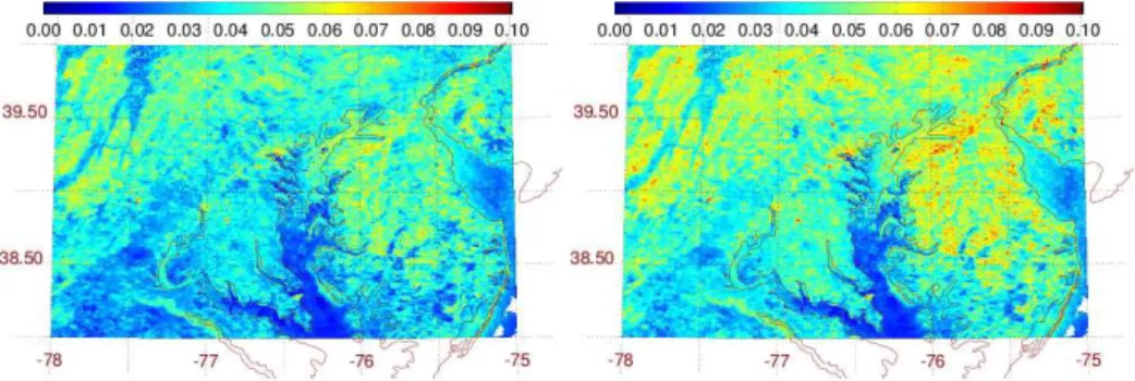
Averaging the BRDF coefficients over an OMI pixel may not be equivalent to averaging the high-resolution surface LER over the OMI pixel. We carried out a numerical ex-periment of calculations of TOA radiances using the high-resolution BRDF coefficients and OMI geometries for the Washington–Baltimore area of the United States (Fig. 1). The TOA radiances were converted into LERs using Eq. (7) and then the LERs were averaged over OMI pixels. The resulting LERs were compared with that calculated from the standard procedure of averaging the BRDF coefficients first. We found that the mean LER difference was equal to 0.75×10⁻⁵with a standard deviation of 4.2×10⁻⁴, which is quite acceptable for our purposes.
geometry-Figure 1.High spatial resolution MODIS-based LERs for the Baltimore–Washington area of the United States for 17 (left) and 18 (right) January 2005 computed with the original spatial resolution of 30 arcsec but for OMI observational geometries.
dependent LER may result in overestimation of the BRDF ef-fects. While non-absorbing aerosols are implicitly accounted for in the cloud algorithms (see Sect. 2.3.1), the aerosols di-rectly affect the AMF, and thus trace-gas retrievals.
Figure 2 shows a data flow diagram that summarizes the generation of the geometry-dependent LER for satellite in-struments. The diagram shows input data, all the steps of processing the data, and outputs. The input data include MODIS-derived land BRDF kernel coefficients and land– water flags, chlorophyll values, terrain heights from a digital elevation model, and wind speed at a height of 10 m. All the input data are averaged over a nominal OMI pixel using the OMI pixel corner information. The averaged input data, OMI pixel geometry, and atmospheric profiles are used to compute the TOA radiance with VLIDORT. The geometry-dependent LER is calculated from the TOA radiance using Eq. (7) and a pre-computed lookup table of radiative transfer parameters. Values of the geometry-dependent LER for each OMI pixel along with ancillary data are written in an HDF5-EOS output file for every OMI orbit.
3 Results and discussion 3.1 Geometry-dependent LER
Because reflection of incoming direct and diffuse solar light from non-Lambertian surfaces depends on satellite observa-tional geometry, the same area observed at different geome-tries can have different LERs. Figure 1 shows the MODIS-based high spatial resolution LER over the Baltimore– Washington area of the United States for 2 consecutive days (17 and 18 January 2005) computed using the OMI observa-tional geometry. The SZA and VZA values are in the similar ranges for both days. However, there is a large difference in the relative azimuth angle, which varies from around 63◦for 17 January to about 118◦for 18 January. Since the land tends to have strong backward scattering, this explains the higher LER for 18 January than that for 17 January. The differences, if not accounted for, may produce errors in the trace-gas re-trievals.
VLIDORT MODIS
(MCD43GF) land BRDF
kernel coefficients
Ocean chlorophyll (2.5 arc min)
Land Water flag map (30 arc sec)
Digital ElevaMon (2 arc min)
OMI pixel-based LER product
LER, BRDF & elevaMon (pixel means and σ), TOA radiances 10m wind
speed (MERRA-2)
OMI pixel sun-satellite
geometry
Atmospheric Profiles (Rayleigh)
LER calculaMon Look up tables of
radiaMve transfer parameters (I0, T, & Sb)
Top-of-atmosphere (TOA) radiance (I comp)
OMI (OMPIXCOR) pixel corners Pixel averaged
parameters (land fracMon, BRDF coefficients, chlorophyll,
elevaMon, wind speed)
BRDF models (land & water)
Figure 2.Data flow diagram of generating the geometry-dependent
LER.
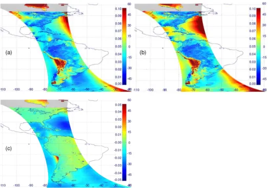
A comparison of the computed geometry-dependent and climatological LERs at 466 nm is shown in Fig. 3 for OMI orbit 12414 of 14 November 2006. The climatological LERs (monthly) are derived from OMI observations (Kleipool et al., 2008). In general, the eastern portion of the orbital swath (that has a later Equator crossing time) has higher values of the LERs than the western part. This is an effect of the OMI observational geometry and BRDF increases in the backscat-tered direction over land. Over the US, the western portion of the orbital swath has higher values of the LER than the eastern portion. This is explained by the dominance of the difference in climatological surface reflectances between the east and the west (see Fig. 3b) as compared with the BRDF increase due to the OMI observational geometry.
cli-Figure 3. (a)LERs computed at 466 nm for OMI orbit 12414 of 14 November 2006 using MODIS-based BRDF with OMI geometry,
(b)OMI-based monthly climatology, and(c)their difference: MODIS-based minus climatological LERs. Missing MODIS BRDF data are
shown in grey here and elsewhere.
matological LERs are affected by residual aerosols. More-over, climatological LERs are inherently contaminated by clouds due to substantially larger sizes of OMI pixels as com-pared with those of MODIS. This is particularly true for the Amazonian region where clouds are persistent.
Over ocean, the geometry-dependent LERs are systemati-cally higher than the climatological LERs in areas affected by sun glint and at large VZAs. This is because the climatologi-cal LERs are based on the mode of LERs from a long time se-ries of observations over a given area; this minimizes the im-pact of observations affected by sun glint and high values that occur at large VZAs. The total ocean reflectance is comprised of three components: direct and diffuse solar light reflected from the ocean surface and water-leaving light. The fraction of each component strongly depends on geometry. Reflection of direct solar light dominates in the sun-glint area. At the edges of the swath the relative contribution of reflected dif-fuse light increases because the sky radiance increases to the horizons and the reflection angle increases thus the Fresnel reflection increases. The higher values of LER nearer to the eastern part of the swath than at the western part are mostly due to sky light reflected from the ocean surface. The angular distribution of the sky radiance is not symmetric in the plane of satellite observations because the sun is in the western part of the swath. The sky radiance is higher in the eastern part of the swath, and it is reflected at higher angles than the light from the western part. Additionally, the higher reflection an-gle results in higher Fresnel reflection in the eastern part of the swath. This is confirmed by our calculations of the view
angle dependence of the reflected light only, i.e., no water-leaving radiance included.
Figure 4 shows the geometry-dependent LERs computed at 466 and 354 nm and their differences for the same OMI orbit 12414 of 14 November 2006. Here, we assume that the BRDF coefficients over land are spectrally independent. The LER differences over land are thus solely due to the smooth-ing effect of enhanced Rayleigh scattersmooth-ing in UV that in-creases the diffuse to direct incident irradiance ratio as com-pared with 466 nm. Over land, LER(354)<LER(466), but the differences are relatively small (<0.015).
Over the ocean, the LER differences additionally result from the spectral dependence of water-leaving radiance. Over the sunglint areas, the solar light reflected from the ocean surface is significantly brighter at 466 nm than at 354 nm, thus leading to higher LERs. Over areas less affected by sunglint, LER(354)>LER(466) in general due to higher amounts of water-leaving radiance.
sun-Figure 4.Similar to Fig. 3 but showing geometry-dependent LERs computed for(a)466 nm,(b)354 nm, and(c)their difference: 466 nm minus 354 nm LER.
Figure 5. (a) RRS-retrieved ECF computed with geometry-dependent LERs and(b) the difference between the ECFs computed with
geometry-dependent and climatological LERs for OMI orbit 12414 of 14 November 2006. ECF data correspond to LER shown in Fig. 4b.
glint geometry. Outside of the regions where OMI observes glint, the LER in the Amazon basin may still be higher than expected due to the turbidity of some rivers in the Amazon floodplain that varies seasonally.
3.2 BRDF effects on the OMI cloud products 3.2.1 RRS algorithm
Figure 5 shows ECFs computed with geometry-dependent LERs and the differences with respect to the climatologi-cal LERs (1ECF) for OMI orbit 12414 of 14 November 2006. The largest 1ECFs (up to 0.05) take place over the less cloudy Amazonian areas.1ECF is obviously lower for cloudy areas due to the diminished effect of surface proper-ties on TOA radiance. The heavily cloudy areas are easily identified on the1ECF map.
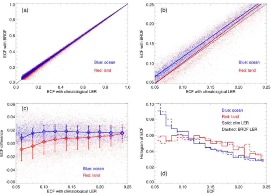
Figure 6a is a scatter plot of ECF retrieved with the geometry-dependent LERs vs. ECF retrieved with clima-tological LERs for the entire range of ECF. It shows that the scatter of data around the 1:1 line diminishes with in-creasing ECF; i.e., the difference in ECFs decreases with increasing ECF as expected. We next examine the most in-teresting range of ECF for trace-gas retrievals, ECF<0.25, which corresponds tofr<0.4–0.5. For this range, Fig. 6b shows a scatter plot of the ECFs retrieved with the geometry-dependent vs. climatological LERs and Fig. 6c shows how
Figure 6. (a)Scatter plot of RRS-retrieved effective cloud fractions (ECFs) computed with geometry-dependent LERs vs. climatological
LERs, where the 1:1 line is in black;(b)similar but for 0.05<ECF<0.25 with linear fits;(c)the mean ECF difference (diamonds) and
standard deviation (error bars) as a function of ECF;(d)normalized histograms of ECF for 0.05<ECF<0.25. Data are for OMI orbit 12414
of 14 November 2006.
Figure 7. (a)RRS-retrieved cloud optical centroid pressure (OCP) computed with geometry-dependent LERs and(b)the difference between
the OCPs computed with geometry-dependent and climatological LERs for OMI orbit 12414 of 14 November 2006.
The standard deviation of1ECF does not depend much on ECF. It is ∼0.01 over ocean and ∼0.015 over land. Even though1ECF is small on average, it can be as large as±0.05 for individual FOVs, which is quite substantial for the low ECF range. Figure 6d shows normalized histograms of ECFs for 0.05<ECF<0.25. The normalized histograms of ECF retrieved with climatological LER and ECF retrieved with BRDF are close to each other. This reflects small differences between the ECFs on average.
Figure 7 similarly shows OCPs retrieved with the geometry-dependent LER and the differences with respect to those retrieved using the climatological LERs (1OCP) for OMI orbit 12414. There are no obvious geographical
Figure 8. Comparison of RRS-retrieved OCPs computed with geometry-dependent and climatological LERs for OMI orbit 12414 of
14 November 2006; data are for 0.05<ECF<0.25.(a)Scatter plot with regression lines;(b)the mean OCP difference and the standard
deviation;(c)normalized histograms of OCP.
3.2.2 O2–O2algorithm
Spatial distributions of the effective cloud fraction and cloud pressure retrieved from O2–O2are quite similar to those re-trieved from RRS (shown in Figs. 5 and 7). That is why we do not show maps of ECF and OCP retrieved from O2–O2. Here we show comparisons of the cloud products retrieved from O2–O2with the geometry-dependent and climatologi-cal LERs for ECF<0.25. Figure 9 is similar to Fig. 6 but for ECF from the O2–O2 algorithm. 1ECF<∼0.03 over land and <∼0.01 over ocean. The histograms of ECF re-trieved with climatological LER and geometry-dependent LER (Fig. 9d) are similar to that from the RRS cloud algo-rithm (Fig. 6d).
Figure 10 is similar to Fig. 8 but for OCP from the O2– O2 algorithm. 1OCP has values up to 200 hPa. The mean
1OCPs are significantly larger for the O2–O2 algorithm as compared with RRS. On average, 1OCP varies from ∼80 hPa at ECF=0.05 to 5 hPa at ECF=0.25 over land.
1OCP is noticeably lower over ocean. The standard de-viation, up to 100 hPa, is also higher than that from the RRS cloud algorithm. The histograms of OCP retrieved from the O2–O2cloud algorithm (Fig. 10c) noticeably dif-fer from those retrieved from the RRS cloud algorithm (Fig. 8c). According to Fig. 10c, lower altitude clouds (with OCP>800 hPa) are observed more frequently over the ocean than over land. For high-altitude clouds (OCP<450 hPa) the situation is reversed: they are observed more frequently over land than over the ocean. Both patterns in the vertical
distri-bution of clouds are much less pronounced in the histograms of OCP retrieved from the RRS algorithm.
Figure 9. (a)Scatter plot of O2–O2-retrieved ECFs computed with geometry-dependent LERs vs. climatological LERs, where the 1:1 line
is in black;(b)similar but for 0.05<ECF<0.25 with linear fits;(c)the mean ECF difference and the standard deviation;(d)normalized
histograms of ECF.
Figure 10. (a)Scatter plot of O2–O2-retrieved OCPs computed with geometry-dependent LERs vs. climatological LERs with linear fits; data
are for 0.05<ECF<0.25.(b)The mean ECF difference (diamonds) and standard deviation (error bars) as a function of ECF.(c)Normalized
histograms of OCP.
Lin et al. (2014) compared ECFs and OCPs derived from O2–O2absorption using the OMI operational algorithm and their own algorithm that makes use of SCDs from the oper-ational algorithm and a set of ancillary parameters that
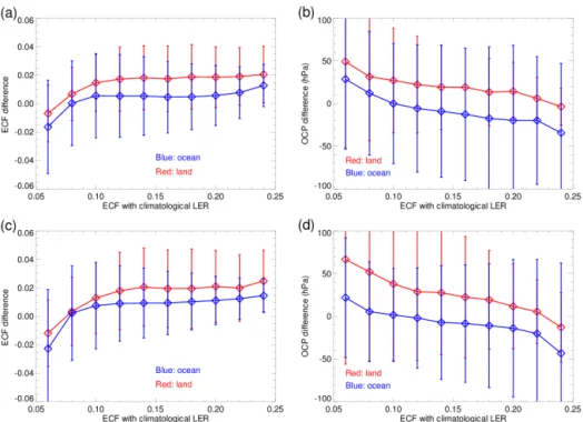
Figure 11. Comparison of O2–O2-derived ECFs and OCPs computed with geometry-dependent and climatological LERs; data are for
0.05<ECF<0.25.(a)The mean ECF difference and(b)OCP difference (diamonds) and standard deviation (error bars) as a function of
ECF for 14 July 2006;(c)the mean ECF difference and(d)OCP difference (diamonds) and standard deviation (error bars) as a function of
ECF for 14 November 2006.
To make the numbers characterizing the ECF and OCP dif-ferences more representative, we processed OMI data for 2 days of 14 November and 14 July 2006. Figure 11 shows the ECF and OCP differences as a function of ECF for those 2 days. The ECF differences calculated for the entire day of 14 November 2006 (Fig. 11c) are close to those calculated for orbit 12414 of that day (Fig. 9b). The OCP differences over land calculated for the entire day (Fig. 11d) are slightly lower than those calculated for orbit 12414 of that day (Fig. 10b), while the OCP differences over ocean for the entire day are quite close to those calculated for one orbit. The ECF and OCP differences are similar for different seasons. A small increase of the OCP differences in November may not be statistically significant. The data in Fig. 11 indicate that the ECF and OCP differences obtained for OMI orbit 12414 are globally representative.
3.3 BRDF effects on the OMI NO2retrievals
We consider the BRDF effect on the NO2 AMFs only, be-cause the retrieved NO2amount is inversely proportional to the AMF. The geometry-dependent LER approach provides an exact match of TOA radiances with the full BRDF ap-proach but not of the photon path lengths. This simplifica-tion can lead to some biases in the calculasimplifica-tion of AMFs and thus to biases in the retrieved NO2 vertical columns. Zhou et al. (2010) have estimated the biases. They compared the box AMFs and NO2vertical columns calculated with the full
BRDF with that calculated with black sky albedo and white sky albedo. According to their data, maximum differences in the box AMFs are up to 10 % at the surface and differences in the NO2vertical columns are smaller than 12 %. We carried out calculations of NO2scattering weights and AMFs with full BRDF treatment and compared them with that calcu-lated with the corresponding geometry-dependent LER. Fig-ure 12a shows an example of the altitude dependence of scat-tering weights calculated with the full BRDF treatment and the geometry-dependent LER. It can be seen that the differ-ence between the scattering weights is small. An AMF dif-ference for this case is 5.6 %. Figure 12b shows a scatter plot of the full BRDF AMFs vs. the geometry-dependent LER AMFs calculated for OMI measurements over the eastern US for orbit 12414 of 14 November 2006. Differences in AMFs due to different treatment of the surface are within±6 % (at 95 % confidence interval) and always less than 10 %.
The tropospheric NO2AMF, AMFtrop, is calculated using the MLER model with input cloud parameters from the O2– O2 algorithm assuming a priori NO2vertical profile shapes (see Fig. 13):
AMFtrop=AMFg(Ps, Rg)(1−fr)+AMFc(OCP, Rc)fr. (8)
The effect of a surface reflectivity change,1Rg, of 0.01 on AMFgis shown as a function ofRgin Fig. 13. The Jacobian,
Figure 12. (a)Scattering weights calculated for an OMI pixel with
the following observation angles: SZA = 53.1◦, VZA = 54.1◦, and
relative azimuth angle RAZ = 60.3◦.(b)AMF calculated with full
BRDF vs. BRDF-derived LER for OMI measurements over the eastern US on 14 November 2006. A regression line is shown in blue. The data are for clear skies.
the lowest atmosphere.J decreases with increasingRgand for unpolluted NO2mixing ratio profiles (Fig. 13).
An effect of replacing the climatological LERs with geometry-dependent LERs on AMFgfor OMI observational geometries and ground resolution can be estimated from Figs. 3 and 13 using 1Rg=LER(BRDF)−LER. The ef-fect is largest over polluted regions in the eastern US, where
1Rgis negative with values from−0.03 to−0.02 (Fig. 3), LER∼0.05, and 1AMFg∼ −20 to−30 %. The BRDF ef-fect reverses over water for glint geometries and large view-ing angles, but Rg is large here and the effect on AMFg is reduced (i.e., small Jacobian).
To estimate the BRDF effect on AMFtrop we need to ac-count for the fr change as well. By differentiating Eq. (8) and assuming that AMFgandfr are independent variables and both depend on1Rg, we get
1AMFtrop =1AMFg(Rg)(1−fr)+1fr[AMFc(OCP, Rc)
−AMFg(Rg). (9)
The cloud AMF strongly depends on the OCP, since high clouds (low OCP) have a shielding effect and low clouds (high OCP), aerosols, and fog can enhance AMFc. Assum-ing a negligible NO2mixing ratio above the cloud OCP, we can neglect AMFcand Eq. (9) simplifies to
1AMFtrop=1AMFg(Rg)(1−fr)−1frAMFg(Rg). (10) Over land, replacing the climatological LERs with the geometry-dependent LERs reduces the surface LER on av-erage (i.e., 1Rg<0), leading to smaller values of AMFg (Fig. 13). At the same time, the mean ECF increases by 0.02 (Fig. 9) and this produces even larger increases infr(1fr∼ 0.04). Therefore both terms in the above equation are neg-ative meaning that switching to a geometry-dependent LER reduces AMFtrop even more over land. The effect is mixed over water, since both1Rgor1frcan change signs for cer-tain geometries. It should be noted that we derived Eqs. (9)
0 2 4 6 8
NO2 [ppb] 1000
900 800 700 600
Pressure [hPa]
(a)
0.00 0.05 0.10 0.15 0.20 Surface reflectivity 0
5 10 15 20 25 30
Changes in tropospric AMF [%]
(b)
Figure 13. (a)November mean NO2profiles at three locations in
the eastern US from the NASA GMI model;(b) air mass factor
(AMF) change due to 0.01 change in surface reflectivity as a func-tion of surface reflectivity. Red: highly polluted profile; green: mod-erately polluted; blue: unpolluted profile.
and (10) to qualitatively illustrate the effect of changing sur-face reflectance on AMF in cloudy conditions. The equations are not used to produce data in the figures of Sect. 3.3. The data in the figures are obtained numerically using Eq. (8).
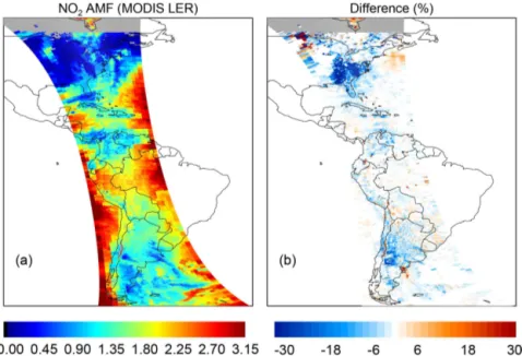
Figure 14 shows that the calculated impact on AMFtrop arising from replacing the climatological OMI-based LERs with geometry-dependent LERs exhibits a strong spatial vari-ation with smaller effects over ocean, unpolluted, or cloudy areas. Over land, where the geometry-dependent LER is gen-erally lower than the climatological LER, use of the BRDF data results in lower AMFs and higher tropospheric NO2 VCDs. The effect is enhanced over polluted areas such as eastern US, where the changes in AMF can reach up to 50 %. The effect is reduced for unpolluted and overcast conditions and mixed over oceans, becauseRgincreases for sunglint and large VZA directions but decreases for other directions.
Figure 14. (a)OMI tropospheric NO2air mass factor (AMF) calculated using geometry-dependent MODIS-based LER;(b)percent differ-ences with respect to climatological LERs for OMI orbit 12414 on 14 November 2006.
Figure 15.Scatter diagrams of AMFs calculated using geometric-dependent MODIS-based LER vs. OMI-based climatological LER for the
orbit 12414 for clear to moderately cloudy sky (fr<0.5) including(a)effects of BRDF only with clouds unchanged and(b)the effects of
both BRDF and O2–O2cloud parameters for land (blue) and ocean (orange). Numbers in parentheses represent percent difference at the 2nd
and 98th percentile range. Percent difference in AMF with changes in surface BRDF and O2–O2cloud parameters, sorting the data by the
difference with respect to(c)LER,(d)OCP, and(e)fr.
Figure 16 illustrates how the use of geometry-dependent LER changes NO2 retrievals over clean and polluted areas. Consistent with previous studies by Lin et al. (2014, 2015), AMFs are considerably lower with geometry-dependent LERs. This suggests that the current operational NO2 prod-ucts based on climatological LERs could be underestimated
Figure 16. AMFs calculated with geometry-dependent
MODIS-based LERs and climatological OMI-MODIS-based LERs over 5◦×5◦
boxes in eastern China (115–120◦E, 36–41◦N; triangle), eastern
US (75–80◦W, 36–41◦N; circle), and South America (55–60◦W,
20–25◦S; plus sign) for clear to moderately cloud skiesfr<0.5.
Orbit 12414 of 14 November 2006 for data over America and orbit 12391 of 13 November 2006 for data over China. AMF calculated with the MODIS-based LER includes the combined effects of
sur-face BRDF and O2–O2cloud parameters. Symbols are color-coded
byfr. Numbers in parentheses represent percent differences at the
2nd and 98th percentile ranges.
4 Conclusions
We developed a new concept of geometry-dependent surface LER and provided a means for computing it. Spatially aver-aged high-resolution MODIS BRDFs are used for computa-tion of the geometry-dependent LER over land for OMI pix-els. The Cox–Munk slope distribution function and the Case 1 water-leaving radiance model are utilized for computation of the geometry-dependent LER over ocean. This method ac-counts for the geometrical dependence of LER within the ex-isting framework of MLER trace-gas and cloud algorithms with only minimal changes. It is important to note that the geometry-dependent surface LER approach can be applied to any current or future satellite algorithms that utilize MLER trace-gas and cloud algorithms.
We examined the effects of the geometry-dependent LER on OMI cloud and NO2algorithms. The effects on retrieved cloud parameters were relatively small on average and dimin-ish with increasing cloud fraction. Even though the impact is small on average, it can be as large as±0.05 for the effec-tive cloud fraction and 100 hPa for the cloud optical centroid pressure. It should be noted that the background aerosols are included in the climatological LER; therefore, they are virtually accounted for in the ECF derived using the LER climatology. The geometry-dependent LER is calculated for aerosol-free conditions; thus the corresponding ECF should
have a bias. The BRDF effects were noticeably higher for the O2–O2algorithm that uses visible wavelengths as compared with the RRS algorithm that utilizes a UV spectral range. This can be explained by the stronger smoothing effect of Rayleigh scattering in the UV as compared with the vis.
We also find that replacing the climatological OMI-based LERs with geometry-dependent LERs can increase the OMI NO2 vertical columns by up to 50 % over highly polluted areas. Only minor changes to NO2columns (within 5 %) are found over unpolluted and overcast areas. It should be noted that the differences include both BRDF effects and biases between the MODIS and OMI-based surface reflectance data sets.
In the future, we plan to implement the use of geometry-dependent LERs in our cloud and NO2 OMI algorithms. Along with the use of the geometry-dependent LER product, we plan to explicitly include aerosols in the NO2algorithm. Further evaluation of the results with OMI data is ongoing. The proposed method of generating the geometry-dependent LERs is computationally expensive. We plan to reduce com-putational cost by using a neural network approach to replace VLIDORT calculations. We also plan to investigate the use of a new surface BRDF product from the Multi-Angle Imple-mentation of Atmospheric Correction (MAIAC) algorithm (Lyapustin et al., 2012).
5 Data availability
The MODIS gap-filled BRDF Collection 5 product MCD43GF used in this paper is available at ftp://rsftp. eeos.umb.edu/data02/Gapfilled/. The OMI Level 1 data used for calculations of the geometry-dependent LER are avail-able at https://aura.gesdisc.eosdis.nasa.gov/data/Aura_OMI_ Level1/. The OMI Level 2 Collection 3 data that include cloud, NO2, and OMI pixel corner products are avail-able at https://aura.gesdisc.eosdis.nasa.gov/data/Aura_OMI_ Level2/.
Competing interests. The authors declare that they have no conflict of interest.
Acknowledgements. Funding for this work was provided in part by the NASA through the Aura science team program. We thank Pawan K. Bhartia for helpful discussions, Ziauddin Ahmad for providing data for comparisons, Andrew Sayer for provision of an updated ocean optics model used in the water-leaving supplement of the VLIDORT code, and Crystel B. Schaaf for consultation on the use of the MODIS BRDF product.
Edited by: F. Boersma
References
Acarreta, J. R., De Haan, J. F., and Stammes, P.: Cloud pressure
re-trieval using the O2–O2absorption band at 477 nm, J. Geophys.
Res., 109, D05204, doi:10.1029/2003jd003915, 2004.
Ahmad, Z., Bhartia, P. K., and Krotkov, N.: Spectral properties of backscattered UV radiation in cloudy atmospheres, J. Geophys. Res., 109, D01201, doi:10.1029/2003JD003395, 2004.
Boersma, K. F., Eskes, H. J., Dirksen, R. J., van der A, R. J., Veefkind, J. P., Stammes, P., Huijnen, V., Kleipool, Q. L., Sneep, M., Claas, J., Leitã, J., Richter, A., Zhou, Y., and Brunner, D.:
An improved tropospheric NO2column retrieval algorithm for
the Ozone Monitoring Instrument, Atmos. Meas. Tech., 4, 1905– 1928, doi:10.5194/amt-4-1905-2011, 2011.
Bucsela, E. J., Krotkov, N. A., Celarier, E. A., Lamsal, L. N., Swartz, W. H., Bhartia, P. K., Boersma, K. F., Veefkind, J. P., Gleason, J. F., and Pickering, K. E.: A new stratospheric and
tropospheric NO2retrieval algorithm for nadir-viewing satellite
instruments: applications to OMI, Atmos. Meas. Tech., 6, 2607– 2626, doi:10.5194/amt-6-2607-2013, 2013.
Chandrasekhar S.: Radiative Transfer, Dover Publications, Inc., NY, 393 pp., 1960.
Cox, C. and Munk, W.: Statistics of the sea surface derived from sun glitter, J. Mar. Res., 13, 198–227, 1954.
Dave, J. V.: Effect of aerosol on the estimation of total ozone in an atmospheric column from the measurements of the ultraviolet radiance, J. Atmos. Sci., 35, 899–911, 1978.
Herman, J. R. and Celarier, E.: Earth surface reflectivity climatol-ogy at 340 to 380 nm from TOMS data, J. Geophys. Res., 102, 28003–28011, 1997.
Joiner, J. and Vasilkov, A. P.: First Results from the OMI Rotational-Raman Scattering Cloud Pressure Algorithm, IEEE T. Geosci. Remote, 44, 1272–1282, 2006.
Joiner, J., Vasilkov, A. P., Flittner, D. E., Gleason, J. F., and Bhar-tia, P. K.: Retrieval of cloud chlorophyll content using Raman scattering in GOME spectra, J. Geophys. Res., 109, D01109, doi:10.1029/2003JD003698, 2004.
Joiner, J., Vasilkov, A. P., Yang, K., and Bhartia, P. K.: Observations over hurricanes from the ozone monitoring instrument, Geophys. Res. Lett., 33, L06807, doi:10.1029/2005GL025592, 2006. Joiner, J., Schoeberl, M. R., Vasilkov, A. P., Oreopoulos, L.,
Plat-nick, S., Livesey, N. J., and Levelt, P. F.: Accurate satellite-derived estimates of the tropospheric ozone impact on the global radiation budget, Atmos. Chem. Phys., 9, 4447–4465, doi:10.5194/acp-9-4447-2009, 2009.
Joiner, J., Vasilkov, A. P., Gupta, P., Bhartia, P. K., Veefkind, P., Sneep, M., de Haan, J., Polonsky, I., and Spurr, R.: Fast simula-tors for satellite cloud optical centroid pressure retrievals; evalu-ation of OMI cloud retrievals, Atmos. Meas. Tech., 5, 529–545, doi:10.5194/amt-5-529-2012, 2012.
Kleipool, Q. L., Dobber, M. R., de Haan, J. F., and Levelt, P. F.: Earth surface reflectance climatology from 3 years of OMI data, J. Geophys. Res., 113, D18308, doi:10.1029/2008jd010290, 2008.
Koelemeijer, R. B. A., Stammes, P., Hovenier, J. W., and de Haan, J. F.: A fast method for retrieval of cloud parameters using oxy-gen A-band measurements from the Global Ozone Monitoring Experiment, J. Geophys. Res., 106, 3475–3496, 2001.
Kuhlmann, G., Lam, Y. F., Cheung, H. M., Hartl, A., Fung, J. C. H., Chan, P. W., and Wenig, M. O.: Development of a custom OMI
NO2 data product for evaluating biases in a regional
chem-istry transport model, Atmos. Chem. Phys., 15, 5627–5644, doi:10.5194/acp-15-5627-2015, 2015.
Lamsal, L. N., Krotkov, N. A., Celarier, E. A., Swartz, W. H., Pick-ering, K. E., Bucsela, E. J., Gleason, J. F., Martin, R. V., Philip, S., Irie, H., Cede, A., Herman, J., Weinheimer, A., Szykman, J. J.,
and Knepp, T. N.: Evaluation of OMI operational standard NO2
column retrievals using in situ and surface-based NO2
observa-tions, Atmos. Chem. Phys., 14, 11587–11609, doi:10.5194/acp-14-11587-2014, 2014.
Levelt, P. F., van der Oord, G. H. J., Dobber, M. R., Malkki, A., Visser, H., de Vries, J., Stammes, P., Lundell, J. O. V., and Saari, H.: The ozone monitoring instrument, IEEE T. Geosci. Remote, 44, 1093–1101, 2006.
Lin, J.-T., Martin, R. V., Boersma, K. F., Sneep, M., Stammes, P., Spurr, R., Wang, P., Van Roozendael, M., Clémer, K., and Irie, H.: Retrieving tropospheric nitrogen dioxide from the Ozone Monitoring Instrument: effects of aerosols, surface reflectance anisotropy, and vertical profile of nitrogen dioxide, Atmos. Chem. Phys., 14, 1441–1461, doi:10.5194/acp-14-1441-2014, 2014.
Lin, J.-T., Liu, M.-Y., Xin, J.-Y., Boersma, K. F., Spurr, R., Martin, R., and Zhang, Q.: Influence of aerosols and surface reflectance
on satellite NO2retrieval: seasonal and spatial characteristics and
implications for NOxemission constraints, Atmos. Chem. Phys.,
15, 11217–11241, doi:10.5194/acp-15-11217-2015, 2015. Lucht, W., Schaaf, C. B., and Strahler, A. H.: An algorithm for the
retrieval of albedo from space using semiempirical BRDF mod-els, IEEE T. Geosci. Remote, 38, 977–998, 2000.
Lyapustin, A., Wang, Y., Laszlo, I., Hilker, T., Hall, F., Sell-ers, P., Tucker, J., and Korkin, S.: Multi-angle implementa-tion of atmospheric correcimplementa-tion for MODIS (MAIAC). 3: At-mospheric correction, Rem. Sens. Environ., 127, 385–393, doi:10.1016/j.rse.2012.09.002, 2012.
Marchenko, S., Krotkov, N. A., Lamsal, L. N., Celarier, E. A., Swartz, W. H., and Bucsela, E. J.: Revising the slant column den-sity retrieval of nitrogen dioxide observed by the Ozone Monitor-ing Instrument, J. Geophys. Res., 120, 5670–5692, 2015. Martonchik, J. V., Bruegge, C. J., and Strahler, A. H.: A review of
reflectance nomenclature used in remote sensing, Remote Sens-ing Reviews, 19, 9–20, 2000.
McLinden, C. A., Fioletov, V., Boersma, K. F., Kharol, S. K., Krotkov, N., Lamsal, L., Makar, P. A., Martin, R. V., Veefkind,
J. P., and Yang, K.: Improved satellite retrievals of NO2
and SO2 over the Canadian oil sands and comparisons with
surface measurements, Atmos. Chem. Phys., 14, 3637–3656, doi:10.5194/acp-14-3637-2014, 2014.
Mishchenko, M. I. and Travis, L. D.: Satellite retrieval of aerosol properties over the ocean using polarization as well as inten-sity of reflected sunlight, J. Geophys. Res., 102, 16989–17013, doi:10.1029/96JD02425, 1997.
Morel, A.: Optical modeling of the upper ocean in relation to its biogeneous matter content (Case I waters), J. Geophys. Res., 93, 10749–10768, 1988.
Noguchi, K., Richter, A., Rozanov, V., Rozanov, A., Burrows, J. P., Irie, H., and Kita, K.: Effect of surface BRDF of various land
cover types on geostationary observations of tropospheric NO2,
Atmos. Meas. Tech., 7, 3497–3508, doi:10.5194/amt-7-3497-2014, 2014.
Nicodemus, F.: Directional reflectance and emissivity of an opaque surface, Appl. Optics, 4, 767–775, 1965.
McPeters, R., Bhartia, P. K., Krueger, A. J., Herman, J. R., Schlesinger, B. M., Wellemeyer, C. G., Seftor, C. J., Jaross, G., Taylor, S. L., Swissler, T., Torres, O., Labow, G., Byerly, W., and Cebula, R. P.: Nimbus-7 Total Ozone Mapping Spectrometer (TOMS) data products user’s guide, NASA Reference Publica-tion 1384, 67 pp., 1996.
Popp, C., Wang, P., Brunner, D., Stammes, P., Zhou, Y., and
Grzegorski, M.: MERIS albedo climatology for FRESCO+O2
A-band cloud retrieval, Atmos. Meas. Tech., 4, 463–483, doi:10.5194/amt-4-463-2011, 2011.
Rienecker, M. M., Suarez, M. J., Gelaro, R., Todling, R., Bacmeis-ter, J., Liu, E., Bosilovich, M. G., Schubert, S. D., Takacs, L., Kim, G.-K., Bloom, S., Chen, J., Collins, D., Conaty, A., da Silva, A., Gu, W., Joiner, J., Koster, R. D., Lucchesi, R., Molod, A., Owens, T., Pawson, S., Pegion, P., Redder, C. R., Re-ichle, R., Robertson, F. R., Ruddick, A. G., Sienkiewicz, M., and Woollen, J.: MERRA: NASA’s Modern-Era Retrospective Anal-ysis for Research and Applications, J. Climate, 24, 3624–3648, doi:10.1175/JCLI-D-11-00015.1, 2011.
Russell, A. R., Perring, A. E., Valin, L. C., Bucsela, E. J., Browne, E. C., Wooldridge, P. J., and Cohen, R. C.: A high
spa-tial resolution retrieval of NO2 column densities from OMI:
method and evaluation, Atmos. Chem. Phys., 11, 8543–8554, doi:10.5194/acp-11-8543-2011, 2011.
Schaaf, C. B., Gao, F., Strahler, A. H., Lucht, W., Li, X., Tsang, T., Strugnell, N. C., Zhang, X., Jin, Y., Muller, J.-P., Lewis, P., Barnsley, M., Hobson, P., Disney, M., Roberts, G., Dunderdale, M., Doll, C., d’Entremont, R., Hu, B., Liang, S., and Privette, J. L.: First operational BRDF, albedo and nadir reflectance prod-ucts from MODIS, Remote Sens. Environ., 83, 135–148, 2002. Schaaf, C. L. B., Liu, J., Gao, F., and Strahler, A. H.: MODIS
albedo and reflectance anisotropy products from Aqua and Terra, in: Land Remote Sensing and Global Environmental Change: NASA’s Earth Observing System and the Science of ASTER and MODIS, Remote Sensing and Digital Image Processing Series, Vol. 11, edited by: Ramachandran, B., Justice, C., and Abrams, M., Springer-Verlag, 873 pp., 2011.
Schaepman-Strub, G., Schaepman, M. E., Painter, T. H., Dangel, S., and Martonchik, J. V.: Reflectance quantities in optical re-mote sensing–definitions and case studies, Rere-mote Sens. Envi-ron., 103, 27–42, 2006.
Seftor, C. J., Taylor, S. L., Wellemeyer, C. G., and McPeters, R. D.: Effect of Partially-Clouded Scenes on the Determina-tion of Ozone, in: Ozone in the Troposphere and Stratosphere, Part 1, Proceedings of the Quadrennial Ozone Symposium, Char-lottesville, USA, 1992, NASA Conference Publication 3266, 919–922, 1994.
Sneep, M., de Haan, J., Stammes, P., Wang, P., Vanbauce, C., Joiner, J., Vasilkov, A. P., and Levelt, P. F.: Three way comparison between OMI/Aura and POLDER/PARASOL cloud pressure products, J. Geophys. Res., 113, D15S23, doi:10.1029/2007JD008694, 2008.
Spurr, R. J. D.: VLIDORT: a linearized pseudo-spherical vector dis-crete ordinate radiative transfer code for forward model and re-trieval studies in multilayer multiple scattering media, J. Quant. Spectr. Ra., 102, 316–421, 2006.
Stammes, P., Sneep, M., de Haan, J. F., Veefkind, J. P., Wang, P., and Levelt, P. F.: Effective cloud fractions from the Ozone Moni-toring Instrument: Theoretical framework and validation, J. Geo-phys. Res., 113, D16S38, doi:10.1029/2007JD008820, 2008. Strahan, S. E., Duncan, B. N., and Hoor, P.: Observationally
de-rived transport diagnostics for the lowermost stratosphere and their application to the GMI chemistry and transport model, At-mos. Chem. Phys., 7, 2435–2445, doi:10.5194/acp-7-2435-2007, 2007.
Thalman, R. and Volkamer, R.: Temperature dependent absorption
cross-sections of O2–O2collision pairs between 340 and 630 nm
and at atmospherically relevant pressure, Phys. Chem. Chem. Phys., 15, 15371–15381, doi:10.1039/c3cp50968k, 2013. Vasilkov, A. P., Kondranin, T. V., Krotkov, N. A., Lakhtanov, G. A.,
and Churov, V. E.: Properties of the angular dependence of po-larization for upward radiation from the sea surface in the visi-ble region of the spectrum, Izvestiya, Atmospheric and Oceanic Physics, 26, 397–401, 1990a.
Vasilkov, A. P., Kondranin, T. V., and Krotkov, N. A.: The effective-ness of polarization measurements in passive remote sensing of the ocean in the visible region of the spectrum, Sov. J. Remote Sens., 7, 886–899, 1990b.
Vasilkov, A. P., Herman, J., Krotkov, N. A., Kahru, M., Mitchell, B. G., and Hsu, C.: Problems in assessment of the UV penetration into natural waters from space-based measurements, Opt. Eng., 41, 3019–3027, 2002.
Vasilkov, A. P., Joiner, J., Yang, K., and Bhartia, P. K.: Improv-ing total column ozone retrievals by usImprov-ing cloud pressures de-rived from Raman scattering in the UV, Geophys. Res. Lett., 31, L20109, doi:10.1029/2004GL020603, 2004.
Vasilkov, A. P., Herman, J., Ahmad, Z., Kahru, M., and Mitchell, B. G.: Assessment of the ultraviolet radiation field in ocean wa-ters from space-based measurements and full radiative-transfer calculations, Appl. Optics, 44, 2863–2869, 2005.
Vasilkov, A. P., Joiner, J., Spurr, R., Bhartia, P. K., Levelt, P. F., and Stephens, G.: Evaluation of the OMI cloud pressures derived from rotational Raman scattering by comparisons with other satellite data and radiative transfer simulations, J. Geophys. Res., 113, D15S19, doi:10.1029/2007JD008689, 2008.
Yang, E.-S., Vasilkov, A., Joiner, J., Marchenko, S., Krotkov, N., Haffner, D., and Bhartia, P. K.: A new cloud pressure
algorithm based on the O2–O2absorption band at 477 nm, OMI
Science Team Meeting, de Bilt, The Netherlands, available
at: http://projects.knmi.nl/omi/documents/presentations/2015/
ostm19/monday/Poster_Vasilkov.pdf, last access: 18 January 2017, 2015.
Zhou, Y., Brunner, D., Spurr, R. J. D., Boersma, K. F., Sneep, M., Popp, C., and Buchmann, B.: Accounting for surface
re-flectance anisotropy in satellite retrievals of tropospheric NO2,