1.Instituto Nacional de Pesquisas Espaciais – São José dos Campos/SP – Brazil 2.Pontifícia Universidade Católica do Rio de Janeiro – Rio de Janeiro/RJ – Brazil 3.Instituto de Aeronáutica e Espaço – São José dos Campos/SP – Brazil 4.Instituto Tecnológico de Aeronáutica – São José dos Campos/SP – Brazil
Author for correspondence: Luciana Bassi Marinho Pires | Instituto Nacional de Pesquisas Espaciais – INPE/CPTEC | Avenida dos Astronautas, 1.758 – Jardim da Granja | CEP 12.227-010 São José dos Campos/SP – Brazil | Email: [email protected]
Received: 13/11/12 |Accepted: 15/05/13
Simulations of the Atmospheric Boundary
Layer in a Wind Tunnel with Short Test
Section
Luciana Bassi Marinho Pires1, Igor Braga de Paula2, Gilberto Fisch3, Ralf Gielow2, Roberto da Mota Girardi4
ABSTRACT: This article presents a study of three different passive devices (spires, screens, and a carpet) separately and in various combinations, to simulate the atmospheric boundary layer (ABL) in a wind tunnel with a short test chamber (465×465x1200mm). The influence of distances between these devices on the formation of the ABL is established, and optimization of variation of thicknesses of the screens (thin, medium, and coarse) on pressure loss is explored. The results obtained in this work gave support for the analysis of the atmospheric flow and turbulence at Alcantara Launching Center (ALC) in order to launch Brazilian space vehicles under safe conditions. The results show that the “spires” and the thin screen are the devices that require the least area to form an ABL in a test chamber. The physical proximity of two devices (the spires and the medium screen) also influences the size of the ABL formed, which varies from 180 to 200 mm. The power law exponent ranged from 0.12 up to 0.14 after the insertion of a carpet.
KEYWORDS: Passive methods, Spires, Carpet, Screens, Wind power law.
INTRODUCTION
within the Brazilian Space Program (Pires et al., 2010). There are several studies using the wind tunnel for simulating the characteristics and behavior of the atmosphere. Some examples are the works of Novak et al.,
(2000) analyzing the turbulent structure of the atmosphere within and above canopies; Kwon et al., (2003) simulating the atmospheric wind field over a complex topography in order to plan the Naro Space Center in South Korea; Mavroidis et al., (2003), studying pollutant dispersion fields immersed in obstacles; Cao and Tamura (2006), simulating the turbulent BL flow over 2D steep, smooth, and rough hills in Tokyo. Kozmar (2009) reproduced the BL at different scales inside the wind tunnel to address the proper choice of simulation length scale and concluded that the length-scale factor does not influence the generated ABL models when using similarity criteria; and recently, Carpentieri et al., (2012) worked to quantify the mean and turbulent flow in geometries of real street canyon intersections, focusing on the area surrounding the intersection between Marylebone Road and Gloucester Place in Central London, UK. Recently, Avelar et al., (2012) did a detailed analysis of the atmospheric flow at ALC using a large wind tunnel. They have constructed the ABL profile using a combination of barrier and small blocks of wood. As all of them used wind tunnels for their experiments, new techniques and methods to develop the ABL are necessary in order to use different sizes of wind tunnel section tests.
The methods of simulating the ABL in wind tunnels are divided into passive and active types. The passive methods use barriers such as grilles, flat plates, triangular plates, writing pads, spires, carpets, etc. The active methods are those that use air jets to form a wall of fluid. The objective of this work is to present some of the passive devices (screens, spires, and carpet) used for the formation of the BL in wind tunnels. It will be done analyzing the optimizations of the formation of the ABL with the use of such devices as a function of both the distance among them and their characteristics (grids with larger or smaller spacing) based primarily on the mean velocity profile and turbulence intensity profiles. The main focus was on rural terrain. However, additional studies could investigate whether this approach works well when applied to other types of terrains (e.g., suburban, urban) with different geometries.
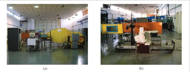
This work was carried out in the commercially available open subsonic wind tunnel Plinth & Partners LDD Wokingham Berkshire England (Serial No. 44/5065 TE) at the Kwein Lien Feng Laboratory at Instituto Tecnológico de Aeronáutica (ITA)/ DCTA, São José dos Campos, SP, Brazil (Fig. 1a). Its test section is square with cut corners (465x465 mm) with a length of 1200 mm. For this study, a channel apparatus with a width of 410 mm and length of 1200 mm, consisting of an uncovered wooden frame, with free edges and side walls parallel to each other and perpendicular to the floor of the wind tunnel, was used to extend the test section for the formation of the ABL. The walls of the tunnel and of the “channel” (Fig. 1b) do not coincide, to minimize the lateral BL of the tunnel. An automatic positioner device with an arm capable of moving in three directions perpendicular to each other and with an accuracy of tenths of a millimeter was used, coupled to a computer, with the data collection points inserted by automatic handling equipment or manually (Fig. 1b). The positioner consists of the following elements: (i) positioner, (“traversing”) from Dantec Dynamics serial code 9057 h 0123, Denmark, (ii) controls for the positioner, Dantec type 57 b 100; and (iii) command manual positioner, serial code 9055X530. The same configuration was utilized by Roballo (2007). The atmospheric flow is simulated by 22 kW (30 hp) electric fans for the range of the windspeeds. The maximum windspeed was 33 m/s (120 km/h).
For initial adjustments, passive devices — screen and spires — were used and for fine tuning a wrinkled carpet was added. It is important to note that the insertion of screens within wind tunnels is usually done with a primary objective of reduction of turbulence of flow, because they have a tendency to uniform the flow and to break the big vortices into smaller ones that decay quickly (energy cascade process). However, in this study, the screens were used to accelerate the formation of the ABL in the test section.
Three types of screens with different meshes were used: (i) nylon square mesh with spacing of 2×2 mm2 and 0.4 mm
in diameter, called “thin screen,” (ii) metal square mesh with spacing of 5.5×5.5 mm2 and 1.0 mm diameter, called “medium
screen”; and (iii) metal mesh type “beehive” with a spacing of 19.0×17.0 mm2 and 0.5 mm in diameter, called “coarse screen”
(Pires, 2009). Details regarding the calculation of the quantity and characteristics of spires that need to be used for different wind tunnel dimensions can be found in Blessmann (1973) and Pires (2009). For this work, three spires, each with heights of 307.7 mm and base width of 32.6 mm, were used. The spires (Irwin, 1981) were produced using steel plates, with each spire consisting of two plates cut and folded together by spot welding (Fig. 3).
Hot-wire measurements were performed with a single-wire BL probe (“Dantec 55P15”) of the constant-temperature hot-wire anemometer (“DANTEC Streamline bridge”). The calibration of the probe was performed using a DANTEC calibration unit. The equipment enables a precise adjustment of flow velocity at the exit of a nozzle. The dynamic pressure of the jet was measured with a standard Betz type manometer, and the respective velocities were correlated with of 2 mm thick. Their tension was adjusted with small plates
used to tighten the mesh to the frame. This was necessary in order to avoid the screen bending from aerodynamic loads during measurements. The mechanism created a small step of approximately 3 mm (approximately 1% of the BL thickness) at the basis of the BL. This height is considered small for the current experiments. For instance, the carpet used to form the ABL had nearly the same height as the step, but a much longer length. Thus, the influence of such a small step on the ABL was assumed to be negligible.
The spires consist of triangular plates arranged in the test chamber entrance which, combined with the surface roughness, are used to generate the windspeed profile of the BL. The dimensions of the spires depend on the desired BL and the dimensions of the tunnel. It is recommended that the distance between two spires should be half of the height of one spire, and their heights should be smaller than the height of the wind tunnel (Pires, 2009). It is assumed, according with Blessman (1973), that the BL real δ
is around 280 m. The tunnel test chamber used has a height of 460 mm and the reduction of scale with respect to the actual size was 1:1000. Therefore it should produce a ABL as close as possible to 280 mm, which was also checked by numerical simulations
Figure 1. Wind tunnel of Prof. Kwein Lieng Feng Laboratory (ITA) (a) and automatic positioner and extension attached (b).
Figure 2. Screens used for the formation of atmospheric
boundary layer. Figure 3. Devices used: carpet, screen, and spires.
Thin screen Medium screen Coarse screen
correction based on the extrapolation of the mean flow data was applied. The procedure resulted in a nearly constant shift of approximately 1 mm. The experimental apparatus is shown in Figs. 4 and 5. It uses an x (longitudinal), y (lateral), and z (vertical) coordinate system to describe the positions of measurements. Hot-wire anemometers of constant temperature were used to measure the flow. These anemometers utilize a several millimeter long tungsten resolution of 16 bits. To avoid clipping effects, the gain applied
to analog signal was fixed; this kept the maximum voltage always below 80% of the range of the AD card. The DC and AC parts of the signal were not split prior to the acquisition; therefore no high-pass filtering was applied. Only low-pass filters were used to avoid aliasing effects. The positioning of the probe was done with a DANTEC traverse mechanism, which provides a resolution of 6.25 μm in all three axes.
spires
410 mm
900 mm
y (mm) screen
x (mm) mesh
300 mm
carpet 20 mm
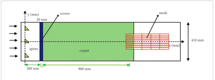
Figure 4. View of the arrangement of the experimental apparatus with the x (longitudinal) and y (lateral) coordinates.
0 -1 0 1 2 2 0
y (mm)
1120
x (mm) 1320
-30 -50 -70
10 30 50 70
1420 1520 1620
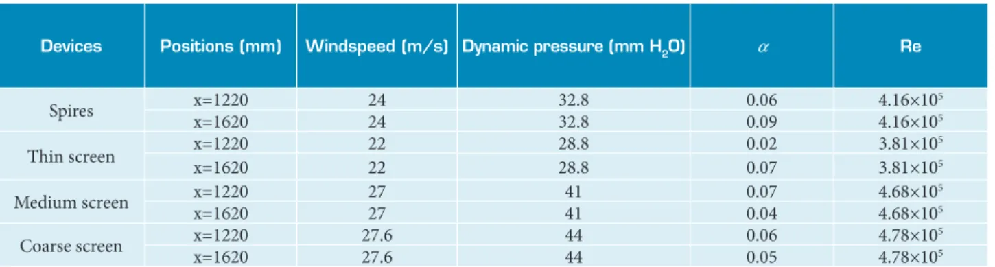
suggested by Pires et al., (2009), and the windspeed used was u∞. The largest pressure loss occurred for the fine screen, with a dynamic pressure of about 28.8 mm H2O and a Re of 3.81×10⁵.
The pressure losses measured by the Pitot tube were smaller for the coarse screen (v=27.6 m/s). The spires presented the second highest pressure loss with Re equal to 4.16×10⁵, which
is not very relevant, since it will be coupled to another device for the generation of the ABL. The ideal configuration causes the smallest pressure loss and generates the ABL in the shortest possible distance of the test section. Note that the coefficient
α is independent of Re or the longitudinal position (x) and is always smaller than 0.1 (ranging from 0.05 up to 0.09). This small value of α is due to absence of other passive devices to fine tune the generation of ABL.
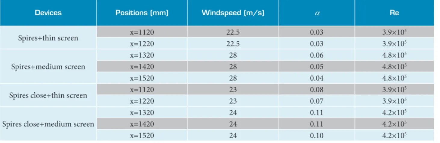
The ABL was fully developed at x=1120 mm, showing nonsignificant differences with the combination of spires and thin screen, due to different gaps between the spires and the screen (150 mm or 300 mm). The combination of the spires with the medium screen moved the ABL to the position x=1420 mm, with the highest mean square deviation for spires 300 mm distant from the screen reaching 3.0 m/s near the surface and 0.5 m/s at the height of 260 mm. For the combination of the spires with coarse screen, the ABL was not developed inside the test chamber section, presenting an irregular windspeed profile, requiring a longer test section for its formation. Table 2 summarizes the values of α and Re for spires combined with the fine and medium screens. The higher values of Re, of about 4.8×10⁵, were obtained for
the medium screen placed further away (300 mm) from the spires. Spires with the thin screen display lower values of Re (3.9×10⁵) for both small and greater separations. The largest
coefficient α occurs for spires close (150 mm) to medium screens, with values around 0.10.
wire with a diameter of around 4 μm. The system functions as one of the resistors in a Wheatstone bridge, allowing measurements with high spatial and temporal resolutions. Further details about this technique can be seen in Roballo (2007). For data acquisition, we used the Labview computer program. The positions on the longitudinal and lateral axes are shown in Fig. 5. The vertical profile was performed at the heights 1, 3, 6, 10, 20, 30, 40, 50, 60, 80, 100, 130, 160, 190, 220, and 260 mm, using a scale factor of 1:1000.
The experimental uncertainty in the measurement of pressure and temperature is 0.1 and 0.4% respectively. This result is an uncertainty of 3.1% in the estimation of the Reynolds number, with the confidence interval of 95%. More details can be found in Roballo (2007).
Initially, the spires and coarse, medium, and fine screen devices were tested separately.
Afterward, combinations of these devices were tested. Then, an optimization of the positions of spires and screen was done with distances of 150 and 300 mm from the screen. Finally, the carpet was inserted to perform the fine tuning of the desired roughness. The metric used to optimize the simulation of rural land was by the coefficient α of the wind power law, which was assumed equal to 0.15.
RESULTS AND DISCUSSION
Table 1 presents the values of the coefficient α of the power law versus the Reynolds number (Re) for the four devices (spires and fine, medium, and coarse screens) individually deployed, corresponding to the positions x=1120 mm and x=1620 mm grid points. Re was calculated for an ABL height of 280 mm as
Table 1. Re and α for isolated spires or screens.
Devices Positions (mm) Windspeed (m/s) Dynamic pressure (mm H2O) α Re
Spires x=1220 24 32.8 0.06 4.16×10
5
x=1620 24 32.8 0.09 4.16×10⁵
Thin screen x=1220 22 28.8 0.02 3.81×10
5
x=1620 22 28.8 0.07 3.81×10⁵
Medium screen x=1220 27 41 0.07 4.68×10⁵
x=1620 27 41 0.04 4.68×10⁵
Coarse screen x=1220 27.6 44 0.06 4.78×10
5
Measurements were carried out at several locations along the stream and spanwise directions, as shown schematically in Fig. 5. The variations of mean and turbulent flow profiles along the spanwise direction were used as a criterion to ensure that the
300 mm
0.2
0.7 0.1
0 0.3 0.4 0.5 0.6 0.7 0.8 0.9 1
(Z
/δ
)
U(z)/U(δ)
0.65 0.75 0.8 0.85 0.9 0.95 1
y = 0
0.02 0
50 100 150 200 250 300
Z
(mm)
ITU/U(δ)
0 0.04 0.06 0.08 0.1 0.12
y = 10 y = 30 y = 50 y = 70
150 mm
0.2
0.7 0.1
0 0.3 0.4 0.5 0.6 0.7 0.8 0.9 1
(Z
/δ
)
U(z)/U(δ)
0.65 0.75 0.8 0.85 0.9 0.95 1 0 0.02
50 100 150 200 250 300
Z
(mm)
ITU/U(δ)
0 0.04 0.06 0.08 0.1 0.12
Figure 6. Nondimensional windspeed and turbulence profile at x=1420 mm. Cases with medium screen (see Table 2). The turbulence level is normalized with respect to the velocity at top of the boundary layer.
Spires+thin screen x=1120 22.5 0.03 3.9×10
x=1220 22.5 0.03 3.9×10⁵
Spires+medium screen
x=1320 28 0.06 4.8×10⁵
x=1420 28 0.05 4.8×10⁵
x=1520 28 0.04 4.8×10⁵
Spires close+thin screen x=1120 23 0.08 3.9×10
5
x=1220 23 0.07 3.9×10⁵
Spires close+medium screen
x=1320 24 0.11 4.2×10⁵
x=1420 24 0.11 4.2×10⁵
x=1520 24 0.10 4.2×10⁵
ABL was developed. Figure 6 shows an example of developed BLs, measured with medium screens. No significant variation of the profiles is present in the results, suggesting the presence of a well-developed flow at position x=1420.
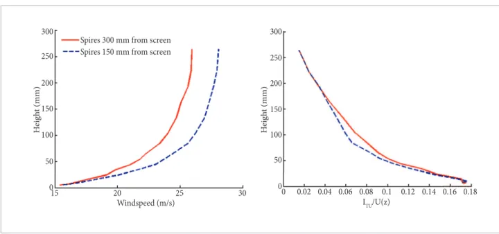
for spires further away from the screen (Fig. 7a), the velocities are greater for low heights, 15 and 25 m/s, respectively.
Figure 8 shows that when the carpet is used in conjunction with screens and spires, the windspeed profiles become more convex, with the greatest convexity noted for the smallest separation between the spires and screens (150 mm).
Figure 7. Windspeed profile at x=1420 mm.
100
50
0 150 200 250 300
H
ei
g
h
t (mm)
Windspeed (m/s)
15 20 25 30
Spires 300 mm from screen Spires 150 mm from screen
100
0.02 50
0 150 200 250 300
ITU/U(z)
0 0.04 0.06 0.08 0.1 0.12 0.14 0.16
H
eig
h
t (mm)
0.18
Figure 8. Windspeed profile and turbulent intensity at the point x=1420 mm with medium screen and carpet.
Figure 7 shows the windspeed profile for a medium screen positioned at 150 mm (named as near) and 300 mm (far) from the spires, with and without the carpet for fine adjustment. Note that the drag is higher with the carpet, and the ABL is better formed with the carpet and a medium screen positioned at a 300 mm distance from the spires. Also,
100
5 50
0 150 200 250 300
H
eig
h
t (mm)
Windspeed (m/s)
0 10 15 20 25 30 35 40
Medium screen distant 300 mm
with carpet without carpet
100
5 50
0 150 200 250 300
Windspeed (m/s)
0 10 15 20 25 30 35 40
assumed to be zero due to the flat terrain conditions and u* and
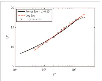
z0 were obtained using the Clauser method. The results of Fig. 9 show a good agreement of the experimental data with the theory. This confirms a good modeling of the mean flow from the ABL at the wind tunnel.
The turbulence intensity is also an important feature of the ABL; therefore its intensities measured in the current experiments were compared to a benchmark suggested by ESDU (Engineering Science Data Unit). Such a benchmark consist of an empirical correlation based on a large experimental database of ABLs measured at height up to 100 m. The expression for this correlation can be found in ESDU (1985) and Liu et al., (2003). Therefore, the current data had to be scaled to the real ABL in order to allow a proper comparison. The results in Fig. 10 show a good agreement between the correlation and the experiments, especially for the streamwise stations where the BL was fully developed (x=1420 and 1520). At these stations, all experimental results lie between the limit of ±15%, represented in the figure Thus, the height of the ABL depends on the distance
separating the devices. Adjusting the data to the theoretical power law profile, with α=0.15, with the spires 300 mm away from the screen, an ABL around 200 mm was obtained, while for the spires closer to the screen (distance of 150 mm), the result was an ABL of 180 mm. The intensity of turbulence showed nonsignificant differences between the two cases.
Table 3 summarizes that Re is not sensitive to the inclusion (or not) of the carpet, varying from 4.2×10⁵ to 4.9×10⁵. However,
the inclusion of the carpet resulted in values of α closer to the ideal 0.15. The height of the ABL increased from 180 to 200 mm as the distance between the spires and the medium screen increased (from 150 to 300 mm). Thus, the mean flow characteristics were apparently met with the combination of spires, medium screen, and carpet. In order to evaluate the results with respect to real ABLs, the mean flow profile was compared to theoretical power law and log-law profiles (Fig. 9). This last one is given by the relation U(z)/u*=1/0.4 log[(z–zd)/z0] (Blessman, 1973), where u* is the friction velocity, z0 is the roughness factor, and zd
is the zero-plane displacement for very rough surface. Here zd is
Y+
Power law - α=0.15
U
+
20
Log law Experiments
15
10
101 102 103
5
Figure 9. Windspeed profile in comparison to theoretical power law (α=0.15) and log law profiles.
Iu
(x=1320)
Z (m)
100
(x=1420) (x=1520)
90 80
0.1 0.2 0.3
70 60
50 40
30 20 10
0
0 0.4 0.5
Figure 10. Turbulent intensity at the first 100 m (equivalent to the boundary layer scaling) and comparison with the correlation suggested by ESDU 7430 and 7431 (Engineering Science Data Unit). The dotted lines represent the ±15% deviation from the correlation.
Without carpet x=1420 28 0.05 4.9×10 –
Without carpet, with spires close to the screen x=1420 24 0.11 4.2×10⁵ –
With carpet x=1420 25.5 0.14 4.4×10⁵ 200
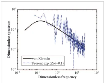
Figure 11. Comparison of the dimensionless spectrum obtained at z/δ=0.1 and the von Kármán spectrum.
to point out that for other terrain conditions, especially those at urban regions, this might not be the case.
CONCLUSION
The ideal situation is the formation of the ABL in the shortest possible extension of the wind tunnel, with the lowest pressure loss possible, to obtain a large Re, similar to the values between 106 and 107 observed in nature. An ABL can be formed
by combinations of passive devices, which do not require a long test section. So, in some situations, existing aeronautical wind tunnels can be used for atmospheric simulations, in particular those with small values of the coefficient α in the power law.
The lowest pressure loss was obtained with the coarse screen alone, while spires followed by a thin screen resulted in the highest pressure loss. The medium screen generated a well-developed ABL at the mesh point x=1420 mm, while the use of thin screen moved the ABL to the position x=1120 mm. In view of these findings, if the length of the wind tunnel is critical (being short) and the pressure loss is not so important; the best choice would be the thin screen.
The distance between spires and screen was the other factor examined. A lower pressure loss, with a larger Re equal to 4.8×10⁵, was observed with the medium screen more distant
from the spires, while for the thin screen Re was equal to 3.9×10⁵. However, higher values of α (equal to or greater than
0.10) were found for all cases of spires closer to the screens. The insertion of a carpet caused a sharp increase of α, which became closer to the desired value of 0.15. The ratio of pressure loss between the distances of the spires and the screen remained the same, but demonstrated a smaller drop with the increase of the distance between the devices; however, for the same screen, the height of the ABL was increased with a smaller distance between the screens and spires, resulting in 180 mm for the distance of 150 mm, and 200 mm for 300 mm.
These findings indicate that this technique is a suitable tool for generation of an ABL in short-chamber wind tunnel experiments. The main characteristics of wind in an ABL seem to be well reproduced in the current experiments. This is confirmed by comparisons with by dotted lines. This suggests that the characteristics of the BL
turbulence were also well modeled at the wind tunnel.
In order to complete the assessment of wind tunnel data, the spectrum of flow fluctuations was compared with the von-Kármán spectrum (ESDU, 1985), and the results are displayed in Fig. 11. According to ESDU, von-Kármán spectrum is a good model to represent the main features of the longitudinal component of turbulence in ABL. The formula of the dimensionless spectrum is fSu/σ2=4X
u(z)/[1+70,78Xu(z) 2]5/6,
where Su is the spectral density function, f the dimensional frequency, σ2 is the variance, and X
u is the dimensionless
frequency. The last term is given by fL(z)/U(z), L(z) being the integral scale calculated using the autocorrelation spectra.
A qualitatively good agreement is found between the experiments and the von Kármán spectrum. The region of constant slope that is equivalent to the -5/3 exponential decay in the inertial subrange of Kolmogorov’s cascade is nearly the same in both cases. Unfortunately, a more quantitative comparison could not be made with the current data because the period set for data acquisition was not long enough to enable the use of averaging procedures. Nevertheless, it is clearly observable that the main features of both spectra are the same. Therefore, it is reasonable to assume that mean flow and the turbulence characteristics of the ABL, expected to occur at the coast close to ALC, could be well simulated in a short wind tunnel with the use of passive devices. It is important
von Kármán Present exp (Z/δ=0.1)
Dimensionless frequency
Dime
ns
io
n
less s
p
ec
tr
um
100
10-1
10-2
100 101 102
10-3
10-2 10-1
flat terrains, which have very small values of power law exponent. For regions with higher terrain roughness, such as forests and urban areas, the ABL wind tunnels clearly are the most suitable tools.
REFERENCES
Avelar, A.C., Brasileiro, F., Marto, A.G., Marciotto, E. and Fisch, G., 2012, “Wind Tunnel Simulation of the Atmospheric Boundary Layer for Study of the Wind Pattern at the Alcantara Space Center”, Journal of Aerospace and Technology Management, Vol. 4, No. 4, doi: 10.5028/jatm.2012.04044912.
Blessmann, J., 1973, “Simulation of the Natural Wind Structure in an Aerodynamic Wind Tunnel” (in Portuguese), Ph.D. thesis, Instituto Tecnológico de Aeronáutica (ITA), São José dos Campos, S.P., Brazil, 169 p.
Cao, S. and Tamura, T., 2006, “Experimental Study on Roughness Effects on Turbulent Boundary Layer Flow over a Two-Dimensional Steep Hill”, Journal of Wind Engineering and Industrial Aerodynamics, Vol. 94, pp. 1-19. doi: 10.1016/j.jweia.2005.10.001.
Carpentieri, M., Hayden, P. and Robins, A.G., 2012, “Wind Tunnel Measurements of Pollutant Turbulent Fluxes in Urban Intersections”, Atmospheric Environment, Vol. 46, pp. 669-674. doi: 10.1016/j. atmosenv.2011.09.083.
Davenport, A.G., 1967, “The Dependence of Wind Loads on Meteorological Parameters”, Proceedings of the International Seminar on Wind Effects on Buildings and Structures, Ottawa, pp. 19-82.
ESDU, 1985, “Characteristics of atmospheric turbulence near the ground. Part II: Single point data for strong winds (neutral atmosphere)”, ESDU International, Item No. 85020, London.
Franck, N., 1963, “Model law and Experimental Technique for Determination of Wind Loads on Buildings”, in Symposium on Wind Effects on Buildings and Structures, Vol. 16, National Physical Laboratory, Teddington, UK, pp. 181-196.
Irwin, H.P.A.H., 1981, “The Design of Spires for Wind Simulation”, Journal of Wind Engineering and Industrial Aerodynamics, Vol. 7, pp. 361–366, doi: 10.1016/0167-6105(81)90058-1.
Jensen, M. and Franck, N., 1963, “Model Scale Tests in Turbulent Wind”, Part I, Danish Technical Press, Copenhagen.
Jensen, M. and Franck, N., 1965, “Model Scale Tests in Turbulent Wind”, Part II, Danish Technical Press, Copenhagen.
Kozmar, H., 2009, “Scale Effects in Wind Tunnel Modeling of an Urban Atmospheric Boundary Layer”, Theoretical and Applied Climatology, Vol. 100, pp. 153–162, doi: 10.1007/s00704-009-0156-3.
141861/2006-1) and a Research Scholarship 302117/2004-0, both
granted by CNPq (Conselho Nacional de Desenvolvimento Científico e Tecnológico, Brazil).
Kwon, K.J., Lee, J.Y. and Sung, B., 2003, “PIV Measurements on the Boundary Layer Flow around Naro Space Center”, Proceedings of the 5th International Symposium on Particle Image Velocimetry, pp. 22-24.
Liu, G., Xuan, J. and Park, S., 2003, “A new method to calculate wind proile parameters of the wind tunnel boundary layer”, Journal of Wind Engineering and Industrial Aerodynamics, Vol. 91, pp. 1155-1162.
Mavroidis, I., Grifiths, R.F. and Hall, D.J.H., 2003, “Field and Wind Tunnel Investigations of Plume Dispersion around Single Surface Obstacles”. Atmospheric Environment, Vol. 37, pp. 2903-2918, doi: 10.1016/S1352-2310(03)00300-5.
Novak, M.D., Warland, J.S., Orchansky, A.L., Ketler, R. and Green, S., 2000, “Wind Tunnel and Field Measurements of Turbulent Flow in Forests. Part I: Uniformly Thinned Stands”, Boundary Layer Meteorology, Vol. 95, pp. 457-495, doi: 10.1023/A:1002693625637.
Pires, L.B.M., 2009, “Study of the Internal Boundary Layer Developed on Coastal Cliffs with Application to the Alcântara Launching Center, Brazil” (in Portuguese), Ph.D. thesis, Instituto Nacional de Pesquisas Espaciais (INPE), São José dos Campos, SP, Brazil. 165p, (INPE-16566-TDI/1562), http://pct.capes.gov.br/teses /2009/33010013003P8/TES.PDF.
Pires, L.B.M., Souza, L.F., Fisch, G. and Gielow, R., 2009, “La Inluencia de la Altura de la Capa Límite Oceánica en la Región del Centro de Lanzamientos de Alcántara en Brasil”, Información Tecnológica, Vol. 20, pp. 119-128, doi: 10.1612/inf.tecnol.4071it.08.
Pires, L.B.M., Roballo, S.T., Fisch, G., Avelar, A.C., Girardi, R.M. and Gielow, R., 2010, “Atmospheric Flow Measurements Using the PIV and HWA Techniques”, Journal of Aerospace Technology and Management, v.2, pp.127-136, doi:10.5028/ jatm.2010.02027410.