ABSTRACT: The present work is concerned with the accurate modeling of transport airplanes. This is of primary importance to reduce aircraft development risks and because multi-disciplinary design and optimization (MDO) frameworks require an accurate airplane modeling to carry out realistic optimization tasks. However, most of them still make use of tail volume coeficients approach for sizing horizontal and vertical tail areas. The tail-volume coeficient method is based on historical aircraft data and it does not consider coniguration particularities like wing sweepback angle and tail topology. A methodology based on static stability and controllability criteria was elaborated and integrated into a MATLAB application for airplane design. Immediate advantages with the present methodology are the design of realistic tail surfaces and properly sized airplanes. Its validation was performed against data of ive airliners ranging from the regional jet CRJ-100 to the Boeing 747-100 intercontinental airplane. An existing airplane calculator application incorporated the present tail-sizing methodology. In order to validate the updated application, the Fokker 100 airliner was fully conceptually designed using it.
KEYWORDS: Aircraft design, Tailplane design, Aircraft stability and control.
An Airplane Calculator Featuring a
High-Fidelity Methodology for Tailplane Sizing
Bento Silva de Mattos1, Ney Rafael Secco1INTRODUCTION
It is of fundamental importance for any optimization framework tailored to airplane design the use of realistic airplane models. If the disciplines that are embedded in the airplane modeling are not accurate enough, it makes no sense performing any optimization tasks, because the resulting planes may be unviable to develop or deliver an acceptable performance. Thus, the present work is concerned with the development of a computational tool able to properly model transport airplane conigurations. An existing computational tool that was christened Aeronautical Airplane (AA) was enhanced with an improved approach for tailplane sizing (Mattos and Magalhães, 2012).
Tail surfaces are used to both stabilize the aircrat and provide control authority that is needed for maneuver and trim. For a conventional aircrat coniguration, the tail oten has two components, the horizontal and the vertical tails. he primary functions of these components are: take care of airplane trim and stability, and provide control by the elevator and rudder surfaces which are associated with the horizontal and vertical tails, respectively.
With regard to aircrat stability, the purpose of horizontal tail (HT) is to maintain the longitudinal stability; while the vertical ones is responsible for keeping the directional stability. Here, we refer to two stability concepts: static and dynamic. Aircrat static stability is deined as the tendency of an aircrat to return to the original trimmed conditions if diverted by a disturbance. Major disturbance sources are gusts and pilot inputs on the controls. On the other hand, the dynamic longitudinal one is related to the motion of a statically stable airplane, the way that it will return
1.Instituto Tecnológico de Aeronáutica – São José dos Campos/SP – Brazil
Author for correspondence: Bento Silva de Mattos | Instituto Tecnológico de Aeronáutica | Praça Marechal Eduardo Gomes, 50 – Vila das Acácias | CEP: 12.228-900 São José dos Campos/SP – Brazil | Email: [email protected]
o
to equilibrium ater sufering some kind of disturbance. Basically, there are two primary forms of longitudinal movements with regard to an airplane attempting to return to equilibrium ater being disturbed. he irst one is the phugoid mode of oscillation, which is a long-period and slow oscillation of the airplane’s light path; the second is a short-period variation of the angle of attack. Usually, this oscillation decreases very quickly with no pilot input (Centennial of Flight, 2011). However, the Centennial of Flight website introduces some misconceptions about Dutch roll, when it states that: “Dutch roll is a motion exhibiting characteristics of both directional divergence and spiral divergence.” herefore, Dutch-roll basic cause is the unbalance between lateral and longitudinal stabilities, when the latter is considerably lower than the irst one.
he tail surfaces of transport airplanes are usually designed to obey static stability criteria. If some undesirable dynamic behaviors become evident during a light test campaign, ixes are provided to overcome the problems. Typical ixes are dorsal and ventral ins, vortex generators, strakes, and in some extreme cases, stablets. he results obtained with an in-house application for tailplane sizing corroborate this statement, as will be shown in the next sections of this work.
As to the controllability topic, it can be stated that an airplane is fully controlled when a flight condition may be changed in a finite time by appropriate control inputs at any new flight condition. In general, a system is considered controllable if it can be transferred from selected initial conditions into chosen final states. The controllability thus describes the influence of external inputs (in general, the controlled variables) to the inner system state. About this, an important distinction must be made between output and state controllability. Output controllability is the notion associated with the system output; the output controllability describes the ability of an external input to move the output from any initial condition to any final one in a finite time interval. No relationship must exist between state and output controllability. The state of a system, which is a collection of its variables values, completely shows the system at any given time. Particularly, no information on the past of a system will help to predict the future, if the states at the present time are known. Complete state controllability (or simply controllability if no other context is given) describes the ability of an external input to move
the internal state of a system from any initial one to any other final in a finite time interval.
Concerning transonic airplanes, tail surfaces should be composed of low-thickness and/or higher sweep than that adopted for the wing, in order to prevent strong shocks on the tail in normal cruise. As required for certiication regulations and safety purposes, transport airplane must dive in an emergency event occurring at high altitudes. he main reason behind this is to reach another one, where no onboard oxygen is needed for the passengers to breath. In this situation, for high-speed airplanes, the airlow over the wing becomes fully detached and the airplane counts just on the horizontal tailplane to depart from the dive. his provides a good reason for airlow remaining attached to HT at this high-speed condition. Former airplane design teams used to increase the HT quarter-chord sweepback angle relative to that igure of the wing (typically a 5 degrees plus). Although providing higher sweepback angles to HT will mean a longer arm relative to center of gravity (CG) and a higher lit curve slope, modern multidisciplinary design and optimization (MDO) frameworks are able to ind out the optimal planform and airfoil shapes for tailplanes. hus, modern design airplanes not necessarily follow the +5 degrees rule to set such angle for the horizontal tail.
In order to keep weight and drag as low as possible, typical values for the maximum relative thickness for both HT and vertical tail (VT) lie in the range of 8 to 11%. Besides working with lower hinging moments, airfoil shapes for the HT shall present a very low maximum camber in order to avoid the generation of undesired induced drag and to maintain interference drag with the tailcone or the VT as low as possible. It is worth mentioning that the tailcone is a region of high decelerating airlow, and the thickness of boundary layer increases fast and dramatically. hus, interference drag is a big issue when integrating conventional HTs into the airframe.
A large variety of tail shapes has been employed on aircraft since the beginning of powered aviation in the early 20th century. These include configurations often denoted by the letters whose shapes they resemble in front view: T, V, H, +, Y, inverted V. The selection of the particular configuration includes complex system-level considerations.
Most of existing MDO frameworks for aircrat design makes use of tail volume coei cient or scaling factors approach for tailplane calculation. A relatively new example of this can be seen in the paper by Grundlach (1999). h e tail volume coei cient approach is based on statistical data and may lead to tailplanes that are unable to comply with stability and controllability requirements. In the present work, a more sophisticated and higher i delity methodology for the design of tail surfaces was compiled from the specialized literature, then coded using MATLAB platform, validated by comparing calculated tail areas to those from some current airliners, and incorporated into an airplane calculator sot ware. Static stability and controllability criteria were used for the design of HTs and VTs of airplanes under consideration.
METHODOLOGY
AiRplAnE CAlCulATOR TOOl
AA is a MATLAB application that calculates transport airplane characteristics, performance, and layout. User must provide to it information regarding geometry, coni guration, topology, wing and tailplanes airfoils, range at given payload, passenger capacity, and engine data of the coni guration that is due to be analyzed.
AA makes use of a wing-body full potential code with boundary-layer correction for wings employing the strip sense approach (Karas and Kovalev, 2011). h is code is known as BLWF and it is able to automatically generate
a multi-block mesh from user-provided coni guration
parameters. h e approximate-factorization algorithm AF2 is used for marching in pseudo time (Holst and h omas, 1982). Aerodynamics coei cients are calculated using Roskam Class II methodology (Roskam, 2000a) and Torenbeek’s formulation to estimate divergence Mach number of wings and HTs (Torenbeek, 1982).
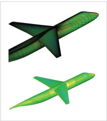
Loads calculations are performed with BLWF for some points in the airplane operational envelope (Fig. 1). At erwards, the calculated loads are used to estimate the wing structural weight applying Megson’s method in some sections of the wingbox (Fig. 2). Elastic deformation is well iteratively, since the loads will vary when the wing deforms (Fig. 3). h e procedure that was adopted for the wing-box sizing is described in Videiro (2012).
Figure 1. A full-potential code that accounts for viscous effects is used by Aeronautical Airplane. It is able to handle both low- and high-wing coni gurations.
Figure 2. Spars and ribs belong to the wing layout dei ned by Aeronautical Airplanefor a coni guration with engines positioned at aft fuselage. The green area shown above indicates availability for fuel storage.
Auxiliary spar Rear spar Outboard flap
Inboard flap
Aileron Front spar
o
Figure 3. Example of wing elastic bending deformation calculated by Aeronautical Airplane.
Figure 4. Aeronautical Airplane output of some fuselage cross sections.
1 .5 1 0 .5 0 -0 .5 -1 -1 .5
Y (m)
X (m)
-2 -1.5 -1 -0.5 0 0.5 1 1.5 2
2
1.5 1 0.5 0 -0.5 -1 -1.5 -2
-2.5 -2 -1.5 -1 -0.5 0 0.5 1 1.5 2 2.5
Y (m)
X (m)
Figure 5. Design diagram of the airplane coniguration being investigated (green circle). Criteria like the second segment climb and rate of climb at initial cruise altitude (ICA) are employed to verify whether the coniguration comply or not with FAR design requirements (Roskam, 2000).
0.4
0.35
0.3
0.25
0.2
0.15
0.1
0.05
0
Cruise Takeoff Landing 2nd segment Missed approach Climb at ICA 300 ft/min
400 450 500 550 600 650 700 750 Wing loading (kg/m2)
T0/W0→ BLWF is also used in conjunction with XFOIL for the
estimation of the CLmax for the coniguration under study. It is used to calculate the maximum lit coeicient of some sections along the wingspan and BLWF estimates the CLmax of the coniguration using those values in the technique of the critical section.
he turbofan engine model employed by AA is described in Loureiro (2008), who developed a generic deck for turbofan engines based on Benson’s work (Benson, 1995). Fan diameter, bypass ratio, fan pressure ratio, engine parts eiciencies, design point, turbine inlet temperature, and overall pressure ratio are some input variables to this model. Typical outputs from the engine module are fuel low and thrust.
AA also defines the fuselage cross section (Fig. 4) and the design diagram, the latter clustering several Federal Aviation Rules (FAR – from the United States), 25 performance conditions together, enabling a better comprehension of thrust and wing loading figures to fulfill requirements (Fig. 5). Scholz (2011) provided several guidelines that were used to define the fuselage cross section as seen in Fig. 4. The methodology that was employed to generate graphs like the one displayed in Fig. 5 is described in Roskam (2000).
AA calculates fuselage geometry, CG envelope, engine thrust and consumption chart, operational envelope, direct operating cost (DOC), payload-range diagram, airplane light mechanics, takeof path, maximum takeof weight (MTOW) with all airplane component weights, engine emissions, and noise signature.
EnhAnCED TAil Sizing mEThOD
Takeoff is a critical condition for tailplanes design, and therefore some relevant aspects of this flight phase are described in the following paragraphs. Figure 6 illustrates the takeoff segments for airplanes. V1 is the takeoff decision speed, VR the rotation speed, VLofvelocity of liftoff, and V2 is the flight speed over a hypothetical 35-feet obstacle. During the initial phase of the takeoff path, the airplane must be accelerated on the ground to VEF, at which point the critical engine must be made inoperative and remain like this for the rest of the takeoff. V1 means the maximum speed in the takeoff at which the pilot must take the first action, such as: apply brakes, reduce thrust, deploy speed brakes, and stop the airplane within the accelerate-stop distance. It also means the minimum speed in the takeoff, following a failure of the critical engine at VEF, at which the pilot can continue it and achieve the required height above the takeoff surface within its distance (Boeing, 2009).
According to FAR 25.149, Vmca is the calibrated airspeed at which:
• critical engine suddenly becomes inoperative;
• control of the airplane is possible to maintain;
• maintain straight light;
• bank angle shall be lower than ivedegrees;
• Vmca may not exceed 1.2 x Vs.
he conditions for determination of Vmca are:
• maximum takeof thrust on remaining engines;
• most unfavorable CG (usually at CG), where the tail moment arm is the shortest);
• aircrat trimmed for takeof (takeof lap setting);
• maximum TOGW;
• most critical takeof conigurations along the light path, except for landing gear retracted.
Vmcais used for determining the minimum VR and V2 . The V2 must also be chosen in order to satisfy the second segment climb requirement. Vmca must be lower than the
V2 and considering its importance for aircraft performance and safety operation, it was calculated after the tail surfaces had been obtained. For this purpose, the methodology elaborated by Cavanaugh (2004) was incorporated in the present work.
The main objective of the present paper was the calculation of the HT and VT areas through a higher fidelity method than that offered by the tail volume approach. In order to accomplish this, static stability and controllability criteria were employed for the design of the horizontal and vertical tails. The VT area is obtained by taking the larger one from that calculated employing both criteria, while the HT area is obtained with the procedure described previously. Stability derivatives that are needed for the calculation of HT and VT areas were obtained according to Roskam’s methodology (Roskam, 1971). Initial estimated values are required in order to start iterative processes for the HT and VT calculation. MATLAB’s fsolve minimization algorithm was employed for the calculation of the tail-planes areas. Indeed, no optimization of the tail-plane areas was carried out with fsolve. This MATLAB tool is used to find out the tailplane areas, because they depend on several parameters and variables such as wing location along the fuselage.
The incorporation of a more sophisticated methodology for the tail-plane sizing into AA poses a more complex task in the interactive process for MTOW calculation. The determination of the CG location is needed not only for the tail-plane area measurement, but also to position the main and nose landing gear, which is also dependent on the overall CG location, which will guide the wing placement in the configuration. The modified AA was employed to calculate the characteristics of an airplane similar to Fokker 100, a 107-seater airliner. By varying the quarter-chord wing sweepback angle, the impact on HT and VT areas was obtained.
BASElinE AiRplAnE
o
hORizOnTAl STABilizER
Design for controllability
he aircrat trim must be guarantee three axes, x, y, and z, namely the lateral, longitudinal, and directional ones, respectively. When the summation of all forces in x direction (such as drag and thrust) is zero and of all moments including aerodynamic pitching moment about y axis is zero, the airplane is longitudinally trimmed.
HT can be installed at airplane tail-cone or on top of vertical tails. Some airplanes like the Piaggio Avanti business turboprop are itted with foreplanes that are located at forward fuselage. Such foreplanes are known as canards.
he HT is responsible for maintaining longitudinal trim and making the forces summations to be zero, by generating a necessary lit and contributing in the summation of moments in y axis. When the summation of all forces in y direction (such as side force) is zero; and of all moments including aerodynamic yawing moment about z axis is zero, the aircrat is said to have the directional trim.
In order to trim longitudinally, we obtained the airplane seen in Fig. 7.
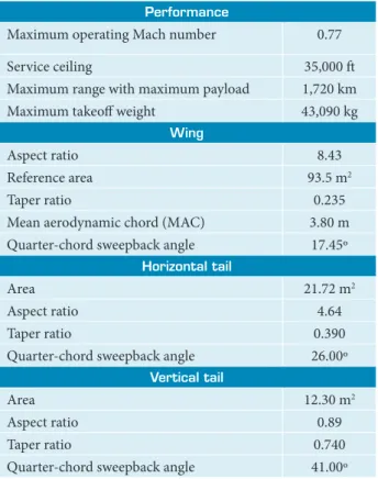
Table 1. Data for the Fokker 100 itted with Tay 620 engines. performance
Maximum operating Mach number 0.77
Service ceiling 35,000 t Maximum range with maximum payload 1,720 km Maximum takeof weight 43,090 kg
Wing
Aspect ratio 8.43
Reference area 93.5 m2
Taper ratio 0.235
Mean aerodynamic chord (MAC) 3.80 m Quarter-chord sweepback angle 17.45º
horizontal tail
Area 21.72 m2
Aspect ratio 4.64
Taper ratio 0.390
Quarter-chord sweepback angle 26.00º Vertical tail
Area 12.30 m2
Aspect ratio 0.89
Taper ratio 0.740
Quarter-chord sweepback angle 41.00º
!
Br a ke releas e
Take-off distance Take-off flight path
Ground roll 1st segment 2nd segment 3rd segment
Final segment
Reference zero
Gear up
1500 ft minimum 400 ft minimum
35 ft (15 ft wet)
One inoperative
Maximum continuous
Final segment speed V2 to final
segment speed
Retracted
Retracted Retraction
Retraction
Enroute climb
Engines
Thrust
Airspeed
Landing gear
High-lift devices V2 V1 VR VLOF V2
0 to V2
Down
Take-off setting Take-off All engines
Segment 1st 2nd Twin-Jet +ve 2.4% Tri-Jet 0.3% 2.7% Quad 0.5% 3.0% Min. climb gradients
xcg-ac Cmac
ach acwf
M0wf l M0h h
Lwf
T
CG W D
Lh
Figure 7. Forces and moments acting for longitudinal trim.
Airplane Type mTOW (kg) Wing area (m2) Overall length (m) hT area (m2) V
h Cessna 172 Light GA
(piston powered)
1,100 16.2 7.9 1.94 0.76
Piper PA-46-350P Light transport (piston powered)
1,950 16.26 8.72 – 0.66
Alenia G222 Military transport (turboprop)
28,000 82 22.7 – 0.85
Fokker 100 Jet airliner (R&R Tay 620)
43,090 93.5 32.5 21.72 1.07
Boeing F/A-18C Fighter 23,400 46 16.8 – 0.49
Pilatus PC-12 Multipurpose single-engine turboprop
4,100 25.81 14.14 – 1.08
Airbus A340-200 Jet airliner 257,000 363.1 59.39 72.90 1.11 Boeing 747-400 Jet airliner 396,830 525 68.63 136.60 0.81 Table 2. Tail volume coeficients for some airplanes (Sadraey, 2009).
(
)
0wf 0h 0e wf cg ac mac h h cg ac mac 0 ( M +M +M +L x − c −L l +x − c = (1)
where xcg-ac is the ratio between the distance of aerodynamic center of the wing to CG and the mean aerodynamic chord of the wing (static margin).
Equation 1 can be further developed and we can obtain Eq. 2:
2 2
0 0
2 w mac wf e Lwf cg ac h 2
V V
S c Cm Cm C x
ρ ρ
η
− −
+ + = −
2 2
0 (2)
2 h 2 h Lhh mac h Lh mac cg ac
V V
S C l c Cm C c x
ρ η ρ
− −
= − +
(2)
Finally, an expression for the area ratio is derived (Eq. 3):
(
)
0 0
0
wf e
h
Lwf cg ac mac h
w h Lh h cg ac mac mac
Cm Cm C x c
S
S η C l x c c Cm
−
−
+ +
=
+ −
(3)
Another form of Eq. 4 is as follows:
0 0 (4
h
wf e wf
h h h L
L cg ac w mac
S l C
Cm Cm C x
S c
η
− ′
= + +
(4)
with Eq. 5:
'
(5)
h h cg ac mac
l =l +x − c (5)
and Cm0h ~ 0, considering that horizontal stabilizers are composed of airfoil sections, which present maximum camber approximately equal to zero.
he combination h h w mac
S l
S c in Eq. 4 is an important
nondimensional parameter for the HT design, and is referred to as the “HT volume coeicient” (Eq. 6). he name is originated from the fact that both numerator and denominator have the unit of volume (e.g. m3). he numerator is a function of HT parameters, while the denominator is of wing parameters (Eq. 6):
h h h
w mac S l V
S c
′
= (6)
Table 2 shows typical Vh igures for some aircrat types. he tail volume coeicient is an indication of handling quality in longitudinal stability and control. As the Vh
increases, the aircrat tends to be more longitudinally stable, and less longitudinally controllable. he ighter aircrat that is highly maneuverable tend to have a very low tail volume coeicient. Transport airplanes require a higher one because they are tailored to perform in a stable light, for passenger and crew’s comfort.
o
serves as a significant parameter both in the longitudinal stability and longitudinal trim issues (Sadraey, 2009). On the other hand, this parameter is usually chosen by looking at similar aircraft. In fact, in the aircraft design, each parameter depends on everything else of the configuration in a non-linear and very complex fashion. In modern conceptual design, MDO frameworks have a commonplace in the aircraft industry (Mattos and Magalhães, 2012). Therefore, the horizontal tail, as well as the vertical stabilizer, shall be designed concurrently with wing and fuselage for a clean and efficient design, and picking up a tail volume coefficient makes no sense anymore.
Design for stability
Another design requirement must be examined: aircrat static and dynamic longitudinal stability. he static longitudinal stability is examined through the sign of the longitudinal stability derivative Cma or the location of the aircrat neutral point; the dynamic behavior is associated with autonomous motions such as Dutch roll, spiral divergence and other issues linked to light quality, which will not be considered in the present work.
For an aircrat with a ixed at tail, the aircrat longitudinal stability derivative is determined as Eq. 7:
(
)
00 2 [ ( )] 1 h f
w wf ac cg h h ac cg
w mac
m d Cm L x x Cm L l x x
V S c dC
Cm d
d
+ + +
= = (7)
Taking into account that, we have Eq. 8:
0h h 1 ,
h L L h h
d
L C C S
d β ε η α = + −
1 1 (8)
wf h h
h h h
m L L h ac cg L h
w w mac
S d S l d
C C C x C
S d S c d
α α α α
ε ε
η η
α − α
= + − − −
(8)
Because the tail operates in the downwash field of the wing (for conventional, aft-tail configurations), the effective tail angle of attack is reduced. According to Roskam (1971), the parameter dε/dα can be estimated by Eq. 9:
(
)
(
)
.19 25 04.44 cos w (9)
w
L M
A h w
L M
C d
k k k
d C α λ α ε α =
= Ψ
(9) where: 1.7 1 1 1 10 3 (10b) A w w w k AR AR
kλ λ
= − + − = − (10a) 1 10 3 ( 7 1 w w w AR AR k z b λ λ − + − = − (10b) 3 7 1 (10c 2 h h h z b k l b λ λ − − − = (10c)
he relationship
(
CLw) (
M/
CLw)
M=0 can be calculated byusing the following expression (Eq. 11):
(
50)
2. . w w L w AR C =
+ + + (11)
When the derivative Cma is negative or the neutral point is behind the aircraft CG, the aircraft is said to be statically longitudinally stable. The limit of the design is found when Eq. 9 is set to zero and therefore Eq. 12 is obtained. ( 1 wf h
L cg ac
h
w h
L h cg ac
mac
C x
S
S d l
C x d c α α ε η α − − = − + (12)
Obtaining the horizontal tail area
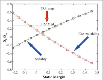
Eqs. 4 and 12 provide two relationships between the area ratio (Sh/Sw ) and xcg-ac. These equations can now be combined into a single graph (Scholz, 2011). It should be observed that the aft center of gravity must be positioned at a safe distance to the natural stability limit. For a jet transport aircraft, Roskam established this value as 5% of MAC. However, according to Raymer (1999), this can be further reduced to 3% of MAC. The permitted areas of focus are now between the limit lines of controllability and those of the stability requirement. Between these lines now, the required CG range can thus be fitted to find out the smallest HT surface area. The region of interest lies above the horizontal green line in Fig. 8.
VERTiCAl STABilizER
Two criteria were adopted for the vertical stabilizer sizing: static stability and controllability. h e i rst condition is related to stability. h e tailplane may be sized to fuli ll a desired coei cient value that incorporates the variation of yawing moment coei cient with yaw angle, Cnβ. h e fuselage and VT are the airplane components that signii cantly impact its directional stability. When an airplane experiences a sideslip angle, in general the fuselage alone will generate a moment that tends to increase the sideslip angle, which is a destabilizing and undesirable condition. h e VT plays a major role to the static directional stability. When the airplane experiences a sideslip angle, the VT has the same aerodynamic ef ects as wings at angle of attack, but at dif erent planes. h us, it generates a moment relative to airplane’s CG, which produces a stabilizing one that tends to neutralize the sideslip angle. h e VT usually has a low aspect ratio, which provides a higher stall angle than high-aspect ratio planforms. If stall occurs, a catastrophic situation may result due to the steady increase of
the sideslip angle. Ventral i ns and stablets are good options to improve Dutch-roll characteristics without an unacceptable weight penalty. h ese surfaces provide a stable yawing moment at larger sideslip angles. h e second consideration for vertical tailplane sizing is associated with controllability. h is criterion may be determinant for a multi-engined underwing coni guration. Loss of power on the number 1 engine, which are numbered from port to starboard, requires that the pilot simultaneously apply right rudder to correct the resulting yaw moment due to asymmetric thrust condition. Also, it should be applied a rolling moment to the right both to hold the starboard wing low and balance the rolling moment due to the rudder. h e low starboard wing produces a side force on the airplane that balances that generated by the rudder del ection.
Engine failure at takeof poses a critical condition for the VT design. In this case, the remaining engine (or engines) must provide enough thrust to maintain the required rate of climb with the additional drag caused by rudder and aileron del ections. Trim drag due to rudder del ection and to a lesser extent aileron del ection may be critical in meeting FAR.121 climb requirements for the second segment, especially for twin-engine airplanes.
An additional vertical tail-sizing requirement, which is harder to calculate, is to keep directional control while on the ground. h e tail must be sized such that the minimum control speed on the ground (VMCG) is less than the takeof decision speed (V1 ). If this is not the case, and VMCG is greater than V1 , then the situation may arise in which critical engine failure occurs above V1 . In such situation, the pilot has to continue the takeof (because V1 has been exceeded), but the airplane lacks adequate lateral control while still on the ground. h e requirements for VMCG are given in FAR 25.149(e). h ey are to lose the most critical engine, apply the rudder (without the use of nose wheel steering), and maintain control down the runway with a maximum of 30 feet (~ 10 m) lateral deviation from the runway centerline. In l ight test, this is performed at successively lower speeds until the pilot can no longer maintain 30 feet lateral deviation. If additional control power is required for a derivative design (such as having increased engine thrust), improved rudder ef ectiveness may be achieved by adding vortex generators to the vertical stabilizer (as was done on the L1011 for one customer with particularly short runway, and reduced Vmca , requirements). If that does not work, a double-hinged rudder might i x the problem. h is was done on the 0.8
0.6
0.4
0.2
0
-0.2
-0.4
-0.6
-0.8
CG range
0.22 MAC
Controllability
Stability
S t a t i c Margin
Sh /Sw
-0.2 -0.1 0 0.1 0.2 0.3 0.4 0.5
Figure 8. Illustration of the calculation procedure for horizontal tail area ratio. Static margin is the variable xcg-ac.
Table 3. CG variation for some airliners (Chai and Mason, 1996, Boeing, 2011).
Airplane Fore/aft
(% mAC)
Variation (% mAC) Boeing 737-800 5/36 31
Boeing 767 11/32 21
Boeing 747-400 8.5/33 24.5 Boeing 777-200 14/44 30
o
In Eq. 15, Vn is the nozzle exit velocity and
Vn/V = 0.92, 0.42 for high- and low-bypass ratio turbofans, respectively. Torenbeek’s wind milling drag equation (Torenbeek, 1982) was validated against the flight test data of 747 (Grasmeyer, 1998). Torenbeek’s equation for the estimation of wind milling drag coefficient shows relatively good agreement with the flight test data over a range of Mach numbers.
h e maximum available yawing moment coei cient is obtained at an equilibrium l ight condition with a given bank angle and a maximum rudder del ection (δr). h e bank angle is limited to a maximum of i ve degrees by FAR 25.149, and the aircrat is allowed to have some sideslip (β) (Grasmeyer, 1998). h e sideslip angle is found by summing the forces along the y-axis:
0 (
y a a y y L
Cδδ +Cδδ +Cββ+C φ=
(16)
We considered in the present work that β = 1 and ϕ is obtained from Eq. 17:
(
)
(1
y y a a
L
C C C
C
ββ δδ δδ
φ= − + +
(17)
Considering that Cyδa ~ 0, Eq. 17 can be simplii ed to Eq. 18:
(
)
(
y
L
C C
C ββ δδ
φ= − +
(18)
If ϕ calculated by Eq. 18 is greater than 50, we set this value for ϕ in Eq. 16 and then β is obtained instead of i xing a value for ϕ. h us, if the pilot slightly increases the sideslip angle further than one degree, he/she will have a safe margin for the increase of the Cn
available. In addition, if one engine is
inoperative, drag could become a critical issue if the sideslip angle were excessively increased.
At er the values for β and ϕ are known, the aileron del ection required to maintain equilibrium l ight is obtained by summing the rolling moments about the x-axis:
0 (1
l a a l l
Cδδ +Cδδ +Cββ =
(19a)
(
l
a
l a
C C
C
δ β
δ
δ β
δ =− −
(19b)
h e rudder del ection is initially set to the given maximum allowable steady state value, and the bank angle and aileron Boeing 747SP (along with increased tail height) to make up
for the shortened fuselage (and thus reduced rudder moment arm), and also on the DC-10.
Design for controllability
h e required yawing moment coei cient to maintain steady l ight with one failed outboard engine at 1.2 times the stall speed is as specii ed by FAR 25.149. h e remaining outboard engine must be at the maximum available thrust, and the bank angle cannot be larger than i ve degrees. Figure 9 shows the engine-out situation for a twin-engine coni guration. h e engine-out constraint is established by constraining the maximum available yawing moment coei cient (Cn
available) to be greater than the required one
(Cn
req) for the engine-out l ight condition (Eq. 13):
Thrust
CG
Drag
lv
le
Figure 9. Engine-out situation of a twinjet airplane.
(
)
(req
windmill e
n
ref w
D T l
C
qS b
+ =
(13)
In Eq. 14, T is the takeof thrust and Dwindmill is the wind milling drag of the failed engine.
h e drag due to the wind milling of the failed engine is calculated using the method described in Appendix G-8 of Torenbeek (1982). h us, we have
(14)
windmill
windmill D ref
D =C qS (14)
where
2 2
2
Re 2
0 07 1
1 0 1
(1 windmill
i n n
i
n D
f
d V V
d
M V V
C
S
+ + =
del ections for equilibrium l ight are determined by Eqs. 19a and b. h e maximum allowable steady-state del ection is typically 20 to 25 degrees. h is allows for an additional i ve-degree of del ection for maneuvering.
h e maximum available yawing moment is found by
summing the contributions due to the ailerons, rudder, and sideslip (Eq. 20):
(
avail (20)
Design for stability
h e remained condition for the design of the vertical stabilizer considers that the airplane is experiencing a sideslip angle (Fig. 10). In this situation, the yaw moment balancing when a sideslip angle is present is enforced
Terms in Eq. 23 are calculated according to Roskam’s methodology (Roskam, 1971):
0 (24)
wing n
Cβ ≅ (25)
(
cos s)
(
VT VT
v v
n y
w
l z
C C
b
β β
α+ α
=−
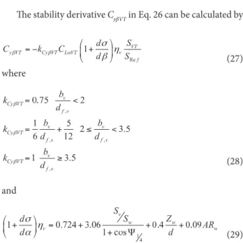
(26)
h e stability derivative CyβVT in Eq. 26 can be calculated by
1 VT (
y VT Cy VT L VT v
f S d
C k C
d S
β β α
σ η β
=− +
(27)
where
,
, ,
,
2
1 v Cy VT
f v
v v
Cy VT
f v f v
v Cy VT
f v b k
d
b b
k
b k
d
= + <
=
(28)
and
1 4
1 0.72 0 0 (
1 c v
w w
w v
S
S Z
d
AR d
d
+ = + + +
+ (29)
In Eq. 30, Zw is a vertical distance between the wing quarter-chord at the location of mean aerodynamic chord and the fuselage centerline, positive downwards.
Eq. 24 is analyzed at the beginning and end of the cruise. h e most critical condition is then considered.
RESULTS
Before integrating the present methodology into an airplane design application, a numerical tool written in
MATLAB®
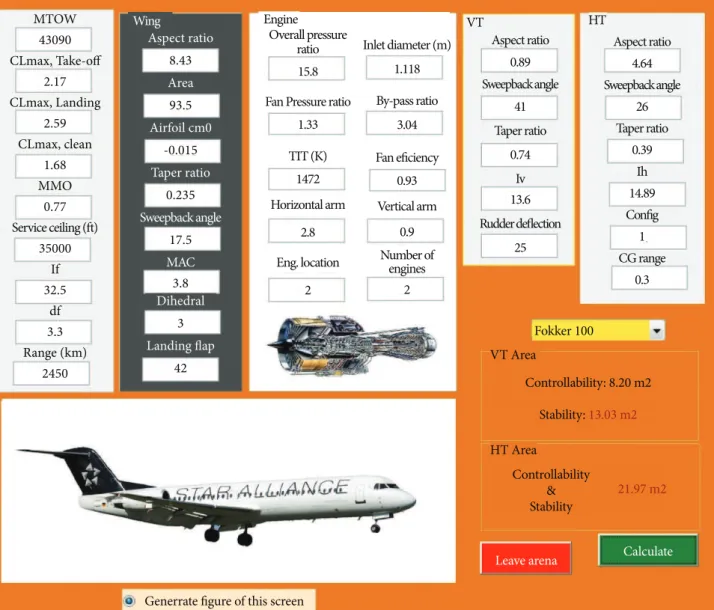
language was developed for tailplane analysis only. The main reason for creating such tool was the validation of the methodology described in the preceding sections. This tool, which was named ITAIL, presents a graphical interface as shown in Fig. 11. Stability derivatives were calculated according to the methods proposed by Roskam (1971). The incorporation of ITAIL into AA will be further described.
Moment caused by fuselage
β
CG
Figure 10. The vertical tail has a stabilizing effect when the airplane is experiencing a sideslip angle.
Re (21)
Eq. 21 can be further developed resulting in Eqs. 22 and 23.
2 2
2 2
e g a l e s u f g
n i w T
V e
n a l p r i
a w n w n w n
n
w (22)
( airplane VT wing fuselage
n n n n
o
Figure 11. Main panel of ITAIL, a tailplane sizing application written in MATLAB
!
®.MT O W 43090 CL m ax , Take-off
2.17 CLmax, Landing
2.59 CLmax, clean
1.68 MMO
0.77 Service ceiling (ft)
35000 If 32.5
df 3.3 Range (km)
2450
Aspect ratio
8.43
Area
93.5
Airfoil cm0
-0.015
Taper ratio
0.235
Sweepback angle
17.5
MAC 3.8 Dihedral
3
Landing flap
42
Wing Engine
Overall pressure ratio
15.8
Fan Pressure ratio
1.33
TIT (K)
1472
Horizontal arm
2.8
Eng. location
2
Inlet diameter (m)
1.118
By-pass ratio
3.04
Fan eficiency
0.93
Vertical arm
0.9
Number of engines
2
VT
Aspect ratio
0.89
Sweepback angle
41
Taper ratio
0.74
Iv 13.6
Rudder deflection
25
HT
Aspect ratio
4.64
Sweepback angle 26
Taper ratio
0.39 Ih
14.89
Config 1
CG range
0.3
Fokker 100
VT Area
HT Area
Controllability: 8.20 m2
Stability: 13.03 m2
Controllability & Stability
21.97 m2
Leave arena
Generrate figure of this screen
Calculate
ITAIL
ITAIL ofers users the possibility of choosing some airliners from a drop-down menu. A broad range of airliners is represented from the regional jet CRJ-100 to the Boeing 747-100. Some characteristics of the airplanes used in the validation process are listed in Table 4. Both T-tail as well as the conventional tail coniguration were considered. Aircrat manufacturers usually bring into market stretched or shortened variants featuring some shared components with a baseline coniguration. Usually, stabilizers are designed for the baseline coniguration in some cases, taking into
account characteristics of the remaining ones. Stretched versions will not be the cause of major concerns because the HT and VT arms will turn these surfaces more efective. However, shortened ones will require larger tailplanes. For this reason, the validation airplanes considered here are baseline conigurations from which others were derived. Most airplane data used for ITAIL validation were taken from online sources (Jenkinson, Simpkin and Rhodes, 2011).
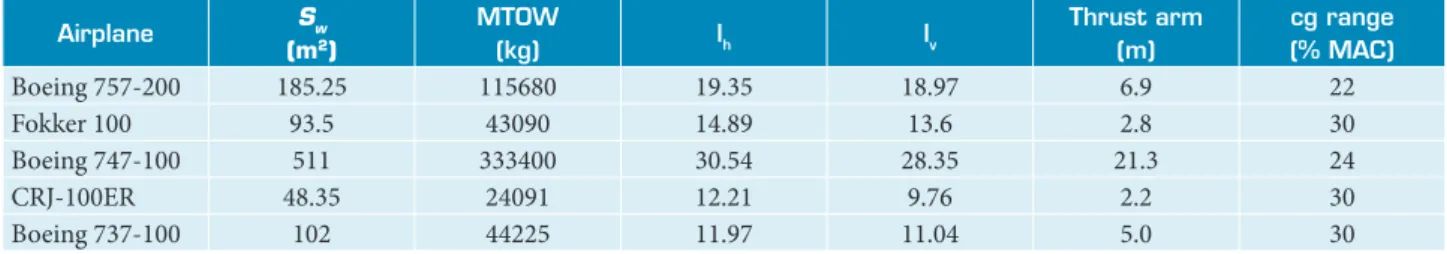
Table 4. Some data belonging to the validation airplanes that were inputted into ITAIL.
Airplane Sw
(m2)
mTOW
(kg) lh lv
Thrust arm (m)
cg range (% mAC) Boeing 757-200 185.25 115680 19.35 18.97 6.9 22
Fokker 100 93.5 43090 14.89 13.6 2.8 30
Boeing 747-100 511 333400 30.54 28.35 21.3 24
CRJ-100ER 48.35 24091 12.21 9.76 2.2 30
Boeing 737-100 102 44225 11.97 11.04 5.0 30
Table 5. Comparison of calculated stability derivatives to experimental data (Boeing 747-100).
Derivative
present work h=12,200 m m=0.90 / α=1.2º
hefley (1972) h=12,200 m m=0.90 / α=2.4º
Cnβ 0.196 0.207
Clβ -0.129 -0.095
Cnδa 0.007 0.0027
Cnδr 0.137 0.0914
Clδr -0.028 -0.0052
Table 6. Calculated tailplane areas for some airliners.
Airplane hT area (m
2) VT area (m2)
Calculated Actual Deviation (%) Calculated Actual Deviation (%)
Boeing 757-200 (RB211-535E4)
52.06 50.35 +3.40 35.61 34.27 +3.91
Fokker 100 (R&R Tay 620)
21.97 21.72 +1.15 13.03 12.30 +5.90
Boeing 747-100 (JT9D-7A)
129.28 136.60 -5.35 77.99 77.10 +1.15
Canadair CRJ-100ER (GE CF34-A)
9.67 9.44 +2.44 9.73 9.18 +5.99
Boeing 737-100 (JT8D-7)
19.46 20.81 -6.50 29.77 28.99 +2.70
Figure 12. Vmca calculation by ITAIL (Boeing 757-200). 1 5 0
1 4 0
1 3 0
1 2 0
1 1 0
1 0 0
9 0
7 7.5 8 8.5 9 9.5 10 10.5 11 11.5
x104
V
M
C
A
(
k
tas
)
vmca vstall
WEIGHT (kg) agreement between calculated and actual igures for the
areas can be considered excellent. he factor that determined the Fokker 100 VT area was stability. Considering that this airplane has at mounted engines, the controllability criterion is not the critical one. A post-design check in order to guarantee that the dynamic stability behavior will be satisfactory is obviously required.
he results presented here corroborates that tailplanes areas of airliners can be usually determined by considering static stability requirements, with undesired dynamic behavior being ixed during light test campaign if needed. Furthermore, design teams should be aware that aerodynamic phenomena like high interference drag, wake vortex and localized low separation can turn tailplanes less efective and this issue must be carefully analyzed. Figure 12 displays the Vmca and stall speed variation with takeof weight for the B-757-200 airliner. he kink in the graph can be credited to the fact that solution for the Vmcacalculation is driven by two kinds of constraints: limitation of rudder or aileron delection. In fact, the lower boundary represents 60.0% of the MTOW and may not be an operating condition.
o
EnhAnCED AEROnAuTiCAl AiRplAnE
Ater ITAIL was validated against HT and VT areas found in a large variety of transport airplane areas, its methodology was incorporated into AA. From this point on, the ability of the enhanced AA to correctly calculate VT and HT areas was put under scrutiny. For this purpose, data of the Fokker 100 airliner were input in that application. Establishing a constraint to the static margin to be exactly 12.5% of MAC, the convergence process to determination of the HT area can be seen in Fig. 13. he parameter XLE in the abscissa axis is the distance from the airplane nose of the wing leading-edge point in the fuselage centerline. Figure 14 reveals the geometry variation and the wing repositioning until the convergence was achieved. AA also provides an artistic view of the inal coniguration, which was displayed in Fig. 14. he HT area that was calculated by AA was 22.1 m2, a deviation of 2.3% when compared to the Fokker 100 actual HT area, which is displayed in Table 5.
he VT area obtained with AA was then 13.6 m2, which obeys three criteria:
• the criterion that Vmca < 1.2 Vs at MTOW, sea level takeof resulted in an area of 6.2 m2;
• the controllability requirement demanded an area of 9.7 m2; and
• the static stability imposed the ultimate area of 13.6 m2 and drove the sizing.
A study about the impact of the variation of the quarter-chord sweepback angle on the tailplane areas was carried out with AA using the Fokker 100 as baseline airplane. he results displayed in Fig. 15 indicated a decrease of the required HT area
31
29
27
25
24
21
30
20
10
0
S
ta
ti
c ma
rg
in (% MA
C)
MT A
re
a (m
2)
XLE (m)
13.1 13.2 13.3 13.4 13.5 13.6 13.7
Figure 13. Static margin and horizontal tail area convergence process for the Fokker 100 airliner.
Figure 14. Above: variation of the coniguration geometry during the convergence process for the horizontal and vertical tails sizing of the baseline coniguration. Wing area and engine data are treated as input variables. Bottom: artistic view of the designed coniguration.
10
5
0
-5
-10
0 5 10 15 20 25 30 35
colors and features a larger horizontal tail than that of the coni guration with higher sweepback angle. h e CG location for the empty airplane and the wing aerodynamic center do not change signii cantly for both coni gurations. AA also provides an output graph of the short period frequency requirements for longitudinal l ight quality in order to verify if the design complies with (Fig. 17).
24
22
20
18
16
14
12
10
A
re
a (m
2)
Quarter-chord sweepback angle 15 20 25 30 35
HI VT
Lower drag force Higher drag force
Resulting restoring moment yawing motion
CG
Figure 15. Above: tailplane area variation with wing quarter-chord sweepback angle of the Fokker 100 airplane. Values were obtained with AA calculator. Bottom: swept-wing airplanes produce a restoring moment improving the directional stability.
Figure 16. Comparison of the HT for the Fokker 100 (green color) and a derived coni guration with 28 degrees of wing sweepback angle.
Figure 17. AA analysis for the Fokker 100, which is represented by the circle between the Level 1 boundaries.
Short Period-Frequency Requirements - Category B Flight Phases
Nza [g 1/rad ]
100 101 102
airplane
Levels 2&3
Level 1 102
101
100
10-1
W
sp
[
rad
1
/s
]
CONCLUDING REMARKS
A MATLAB®
application called ITAIL was developed to validate a methodology for vertical and HT sizing of transport airplanes. ITAIL employs static stability and controllability criteria for tailplane design. h e highest deviation found by the ITAIL application was that for the Boeing 737-100 HT area, i.e. 6.5%. h e agreement between calculated and actual i gures for the areas can be considered excellent. A post-design check in order to guarantee that the dynamic stability behavior will be satisfactory is required. h e results presented here corroborates that tailplanes areas of airliners can be usually determined by considering static stability and controllability requirements,, with undesired dynamic behavior being i xed during l ight test campaign if necessary.
o
LIST OF SYMBOLS
AR = Aspect ratio b = Span
cmac = Mean aerodynamic chord
CL = Lift coeficient
CLα = Variantion of the lift coeficient with angle of attack
CLmax = Maximum lift coeficient of wing or airplane coniguration
Cme = Moment coeficient due to engine
Cm0 = Moment coeficient
Cm0wf = Moment coeficient of the wing - body combination d = diameter
D = Drag force
M∞ = Freestream Mach number
MAC – Mean aerodynamic chord l = length
L = Lift force q = Dynamic pressure S = Area
T = Engine thrust V = Velocity W = weight
α = Angle of attack b = Sideslip Angle
ε = Downwash angle at horizontal tail
h = Ratio between local and freestream dynamic pressure f = Bank angle
r = Air density Ψ = Sweepback angle
SUBSCRIPTS
50 Half chord ac Aerodynamic CG Center of gravity e Engine h Horizontal tail
mca Minimum control speed in the air mcg Minimum control speed in the ground ref Reference (area, length, etc…) s Stall
w Wing ∞ Freestream An existing airplane calculator designated AA was
enhanced with a higher idelity approach for sizing horizontal and vertical tailplanes. AA is a MATLAB application tailored to be incorporated into MDO frameworks. Results obtained with AA using the methodology described in this work and incorporated by ITAIL revealed an excellent agreement
with the VT and HT areas of the Fokker 100 airliner itted with Rolls&Royce Tay 620 engines.
Vmca may become an important driver for the design of the VT if takeof ield length or climb requirements in second segment are very stringent. Both ITAIL and AA applications already consider
Vmca for the VT sizing.
REFERENCES
Benson, T.J., 1995, “An Interactive Educational Tool for Turbojet Engines”, Cleveland, Ohio, NASA Lewis Research Center.
Boeing Co., 2009, “Takeoff Performance”, Boeing Electronic Training Material, Seattle.
Cavanaugh, M.A., 2004, “A MATLAB m-File to Calculate the Single Engine Minimum Control Speed in Air of a Jet Powered Aircraft”, VMCmav1.m User’s Manual, Virginia Tech, VA.
Centennial of Flight, “Dynamic Longitudinal, Directional, and Lateral Stability,” Retrieved on November 12 2011, from http://www.centennialoflight. gov/essay/Theories_of_Flight/Stability_II/TH27.htm
Chai, S.T. and Mason, W., 1996, “Aircraft Landing Gear Integration in Aircraft Conceptual Design”, MAD Report, MAD 96-09-01, Virginia, September.
Grasmeyer, J., 1998, “Stability and Control Derivative Estimation and Engine-Out Analysis,” Virginia Tech Department of Aerospace and Ocean Engineering Report, VPI-AOE-254.
Grundlach IV, J.F., 1999, “Multidisciplinary Design Optimization and Industry Review of a 2010 Strut-Braced Wing Transonic Transport,” Master of Aerospace Engineering Thesis, Virginia Polytechnic Institute and State University, Blacksburg, Virginia.
Hefley, R.K. and Jewell, W.F, 1972, “Aircraft Handling Qualities Data”, NASA CR 2144.
Holst, T.L. and Thomas, S.D., 1982, “Numerical Solution of Transonic Wing Flow Fields”, AIAA paper # 82-105.
Jenkinson, L., Simpkin, P., Rhodes, D., 2001, “Civil Jet Aircraft Design”, Retrieved on November 2 2011, from http://www.elsevierdirect.com/ companions/9780340741528/case-studies/default.htm
Karas, O.V. and Kovalev, V.E., 2011, “BLWF 28 User’s Guide”, Moscow.
Loureiro, V., 2008, “Optimal design of Transport Airplane with a Realistic Engine Model in the Loop,” Undergraduation Thesis, Instituto Tecnológico de Aeronáutica, São José dos Campos, Brazil.
Mattos, B.S. and Magalhães, P.E.C.S., 2012, “Conceptual Optimal Design
of Airliners with Noise Constraints”, 50th Aerospace Sciences Meeting and
Exhibit, Nashville, TN.
Raymer, D.P., 1999, “Aircraft Design: A Conceptual Approach”, 3rd Ed,
Washington D.C., AIAA.
Roskam, J., 1971, “Methods for Estimating Stability and Control Derivatives of Conventional Subsonic Airplanes,” Roskam Aviation and Engineering Corporation, Lawrence, Kansas.
Roskam, J., 2000a, “Airplane Design, Part I: Preliminary Sizing of Airplanes,” The University of Kansas, Lawrence, DARcorporation.
Roskam, J., 2000b, “Airplane Design, Part VI: Preliminary Calculation of Aerodynamics, Thrust and Power Characteristics,” The University of Kansas, Lawrence, DARcorporation.
Sadraey, M., 2009, “Aircraft Performance Analysis,” Verlag Dr. Müller.
Scholz, D., 2011, “PreSTo - Aircraft Preliminary Sizing Tool – From
Requirements to the Three-view Drawing”, EWADE 2011 – 10th Workshop
on Aircraft Design Education, Naples, Italy, May.
Toreenbeek, E., 1982, “Synthesis of Subsonic Airplane Design,” Delft University Press, Delft, the Netherlands.
Videiro, P.L., 2012, “Wing Structural Optimization in Aircraft Conceptual Design,” undergraduation thesis, Instituto Tecnológico de Aeronáutica, São José dos Campos, Brazil.