After 10 years, how do changes in
asset ownership affect the
Indicador
Econômico Nacional
?
Fernanda EwerlingI, Aluísio J D BarrosI
I International Center for Equity in Health. Programa de Pós-Graduação em Epidemiologia. Universidade Federal de Pelotas. Pelotas, RS, Brasil
ABSTRACT
OBJECTIVE: Our main objective was to analyse how the evolution of household assets ownership afected the Indicador Econômico Nacional (IEN – National Wealth index) and to point out the most stable assets and which lost importance more quickly.
METHODS: We analysed the trend of the ownership of each IEN variable and the distribution of the households’ scores. We calculated the correlation coeicients of each variable separately with the IEN score and the household income. We also evaluated how the changes of the score distribution over time afected the validity of the published reference cut-points. We used data from consortium surveys conducted every two years from 2002 to 2014 in the city of Pelotas, Brazil.
RESULTS: An increase in the educational level of household heads and in the ownership of all IEN assets, except radio and telephone, was observed in the study period. In general, the correlation of the assets with the IEN scores decreased over time. here was an increase in the score, with a consequent increase in the quintiles cut-points, but the distance between these cut-points had no signiicant variation. hus, the reference cut-points for Pelotas, quickly became outdated. CONCLUSIONS: Some assets showed greatly reduction on its importance for the indicator, and the reference cut-points became obsolete very quickly. It is essential for a standardized wealth (or asset) index with research purposes to be updated frequently, especially the cut-points of reference distribution.
DESCRIPTORS: Economic Indices. Social Conditions. Social Values. Socioeconomic Analysis. Correspondence:
Fernanda Ewerling
Rua Marechal Deodoro, 1160 Centro
96020-220 Pelotas, RS, Brasil E-mail: [email protected]
Received: 30 Jun 2015 Approved: 11 Dec 2015
How to cite: Ewerling F, Barros AJ. After 10 years, how do changes in asset ownership affect the Indicador Econômico Nacional? Rev Saude Publica. 2017;51:10.
Copyright: This is an open-access article distributed under the terms of the Creative Commons Attribution License, which permits unrestricted use, distribution, and reproduction in any medium, provided that the original author and source are credited.
INTRODUCTION
Social epidemiology sustains that individuals’ health directly connects to their life conditions1.
Its consolidation led epidemiological studies to include socioeconomic determinants
investigation in their analyses2.
Individuals can be classiied in several ways according to their socioeconomic status. Income
and consumption indicators require long questionnaires for their proper determination. As their measurement is not the focus of health surveys, their use in these surveys is generally
not possible4. hus, researchers might choose carefully the most appropriate method for
every speciic situation, considering their strengths and limitations3.
A proxy for household wealth based on household assets and household characteristics (such
as number of bedrooms) was proposed as an alternative5. he called wealth index (or asset
index) is a practical way to classify the households according to their socioeconomic status. It was initially used in the Demographic and Health Survey (DHS), which lacks information on income and consumption. Instead of the current income, this indicator represents the
permanent consumption capacity of the familya. Its main advantage is to rely on a limited set
of variables that are easily collected in health surveys, even with low educated populations. It is also a more stable socioeconomic measure than current income, which is subject to
signiicant luctuations when recorded in a relatively short reference periodb.
he Indicador Econômico Nacional (IEN – National Wealth index) was developed using the same approach of the DHS Wealth Index and is widely used in epidemiological research in
Brazil6-9. Its use enables to calculate scores for households from information on the ownership
of a set of assets, household characteristics and the household head’s education2. he Critério
Brasil, developed by the Associação Brasileira de Empresas e Pesquisas (ABEP), also present a
similar proposal. he IEN is advantageous because it is based on a national coverage sample
and because it provides the reference distribution of scores for Brazilian capitals, states and large regions, as well as the national distribution. From these data, we can compare the study sample (e.g. sample of health care users of the Family Health Strategy) with the more
suitable reference distributionc.
he wealth indices also have important limitations. Its result is a relative measure, which provides a ranking of the individuals, but does not allow the comparison between diferent populations. his is caused by the fact that an individual from the poorest quintile of a high-income country may be richer than one from the richest quintile of a middle or low-income country4. he reference distributions proposed with the IEN was an attempt
to minimize this problem. he use of asset ownership information in the indicator composition, while making the classiication more practical, may be a problem in a
society experiencing rapid income and technology improvements since expensive assets
soon become popular. hus, periodic updates are required to avoid these indicators from
losing discriminatory power.
In the last decades, Brazil experienced a systematic decrease in income inequality, with
especially growth of the poorest families’ income and credit expansiond. Data from the
“Pesquisa de Orçamento Familiar” budget survey showed a popularization of durable
goods. hat is, the poorer families also achieved access to these goods10. he country also
experienced rapid expansion of access to mobile telephony, and the service became almost
universal. he richest strata changed from ixed to mobile telephones11.
As the IEN was created from the 2000 Census data, the relative weights of the assets that compose the indicator probably have changed due to the country’s advances in that period.
his study aimed to analyze the trends of the IEN assets ownership and describe how these changes afected the discriminatory power of the indicator. his will enable to identify the
best types of assets or household characteristics to include in these indicators, favoring those that are more stable and avoiding those that lose importance more quickly.
a Ferguson B, Gakidou E, Murray C. Estimating permanent income using indicator variables.Geneva: World Health Organization; 2003 [cited 2015 Jun 22]. Available from: http://www.who. int/healthinfo/paper44.pdf b Liverpool-Tasie LS, Winter-Nelson A. Asset versus
consumption poverty and poverty dynamics in the presence of multiple equilibria in rural Ethiopia. Washington (DC): International Food Policy Research Institute; 2010 [cited 2015 Jun 22]. Available from: https://www.ifpri.org/publication/ asset-versus-consumption- poverty-and-poverty-dynamics-presence-multiple-equilibria-rural c Associação Brasileira de Empresas de Pesquisa (ABEP). Critério Brasil. São Paulo (SP); 2015 [cited 2015 Jun 22]. Available from: http://www.abep. org/criterio-brasil
METHODS
his study is part of a research consortium conducted in 2014 in the urban area of Pelotas12,
a medium-sized Brazilian municipality in the southern region, which comprehended several
research topics. We also used data from 2002 to 2012 consortium surveys conducted in the same city. IEN was developed in 2005, so the 2002 and 2004 surveys lack information on the
ownership of some IEN assets. herefore, some analyses excluded those years. he target population of all consortia prior to 2014 was adults (≥ 20 years) living in the urban area of Pelotas, except for 2012, which also included adolescents. he older adults (> 60 years) health was the focus in 2014. herefore, the logistics was diferent from the previous years for the
data collection in the households with no older adults.
In all surveys, the sampling process happened in two stages: systematic selection of the census tracts according to the average household head’s income, with probability proportional to
the tract’s size, followed by systematic household selection13. Due to the lack of income
data in 2012, the average education of the household head was used to order the sectors to procced the sampling.
In 2014, a sample size calculation evaluated the proportion of households that owned
each IEN component asset. he refrigerator obtained the largest sample size, with a 99.0% expected prevalence, using alpha error of 5.0% and power of 80.0%. We used a conidence
limit of 0.5 percentage points. According to calculations made in the OpenEpie program,
1,519 households were necessary, of which 506 with and 1,013 without older adult residents.
As the 2014 consortium included only households with older adults, we initially applied a short questionnaire to collect basic information on the household residents (family composition questionnaire). One in every two households without older adults was selected to answer a questionnaire about the ownership of some household assets and household characteristics.
We interviewed 1,937 domiciles (897 with and 1,040 with no older adults). We applied a weight to
each household, equal to the inverse of the sampling probability: 1 was the weight for households
with older adult residents; and 1/(a/b) for the other households, where a is the number of
households with no older adults that were selected for the asset ownership questionnaire and b
is the total number of households with no older adults among those selected in the tract.
A trained team conducted the interviews. In 2014, the interviewers and the ield supervisors
applied the questionnaire of asset ownership to households with no older adult residents,
when these households were identiied by the application of the family composition
questionnaire. We considered losses and denials the interviews unaccomplished after at
least three attempts on diferent days and times. A ield supervisor performed the last
attempts. To control data quality, inconsistencies were checked on a weekly basis and a
reduced questionnaire with key questions was applied in a new supervisors’ visit to 10.0%
of randomly selected interviewees.
The IEN component variables were: household head’s education (in years of study:
0-3/4-7/8-10/11 or more, incomplete higher/complete education); number of bedrooms;
number of bathrooms (with shower and toilet); number of television sets (0/1/2/3+); number of vehicles (0/1/2+); ownership (yes/no) of assets: radio, refrigerator, DVD or video tape (VCR), freezer/duplex refrigerator; washing machine (a cheaper option of washing machine with less
functions, called “tanquinho”, was excluded), microwave, telephone line, computer and air
conditioner. We also analyzed vacuum cleaner, clothes dryer, dishwasher, portable computer,
motorcycle, and internet (broadband or dial-up), pay television (yes/no) and housekeepers.
We assessed the time trend of the ownership of each IEN component variables, as well as the
household scores using descriptive statistics and graphical analyses. he correlation between
each IEN component and (1) the total household scores; and (2) the household income was
calculated. he Research Ethics Committee of the Faculdade de Medicina da Universidade Federal de Pelotas approved this study and the mentioned surveys (Protocol 472.357/2013).
All interviewees signed the informed consent form. e Dean AG SK, Soe MM.
RESULTS
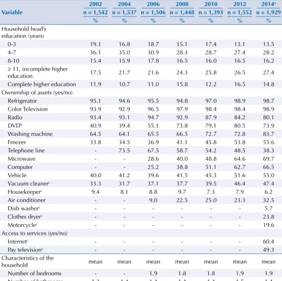
Table 1 shows the increase in the level of the household heads’ education from 2002 to 2014.
In 2002, 29.4% of the household heads had at least complete high school; in 2014, it increased to 42.2%. he number of bathrooms and bedrooms remained relatively constant. he ownership of radios decreased, while the televisions sets increased. he proportion of households with at least one car had no diference between 2002 and 2008, but increased since 2010. he ownership
of refrigerator, freezer, washing machine, microwave, computer, air conditioner and vacuum cleaner increased in the period. In 2014, computer was disaggregated in desktops and portable computers. We found that notebooks/netbooks were already more prevalent than desktops
(49.0% and 41.0%, respectively). DVD (or VCR) ownership increased from 2002 to 2012, but declined in 2014. Fixed telephone lines and housekeepers were diminishing. In 2014, 5.7% of the households had dishwashers, 23.8% had clothes dryers, and 19.6% had motorcycles. In addition, 60.4% and 49.3% of them had internet access and pay television in 2014, respectively. he household characteristics, as well as the household head’s education and the number
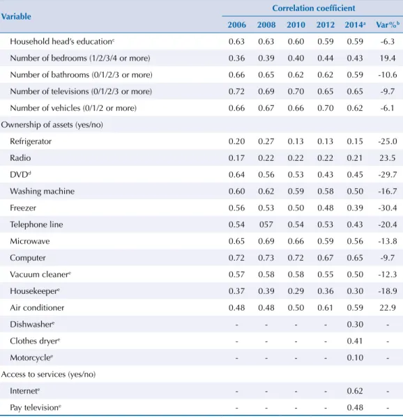
of televisions and vehicles had a stable correlation with the IEN in the period (Table 2). Refrigerator, freezer and DVD were the variables with the greatest decrease in this correlation. Number of bedrooms, radio and air conditioner showed positive variation. Radio did not present a trend of decreased, only a lower correlation in 2006 compared to the following years.
Internet, presented the highest correlation with the indicator, but was irst collected in 2014.
Table 1. Time trends of the household head’s education, assets ownership, access to services and characteristics of the households. Pelotas, RS, Southern Brazil, 2002 to 2014.
Variable
2002 2004 2006 2008 2010 2012 2014a
n = 1,542 n = 1,537 n = 1,506 n = 1,448 n = 1,393 n = 1,552 n = 1,929
% % % % % % %
Household head’s education (years)
0-3 19.1 16.8 18.7 15.1 17.4 13.1 13.5
4-7 36.1 35.0 30.9 28.3 28.7 27.4 28.2
8-10 15.4 15.9 17.8 16.5 16.0 16.5 16.2
≥ 11, incomplete higher
education 17.5 21.7 21.6 24.3 25.8 26.5 27.4
Complete higher education 11.9 10.7 11.0 15.8 12.2 16.5 14.8 Ownership of assets (yes/no)
Refrigerator 95.1 94.6 95.5 94.8 97.0 98.9 98.7
Color Television 93.9 92.9 96.5 97.9 98.4 98.4 98.9
Radio 93.4 93.1 94.7 92.9 87.9 84.2 80.1
DVDb 40.9 39.4 55.1 73.8 79.1 80.5 73.9
Washing machine 64.5 64.1 65.5 66.5 72.7 72.8 83.7
Freezer 33.8 34.5 36.9 41.1 45.8 53.8 55.6
Telephone line - 73.5 67.5 58.7 54.2 48.5 38.3
Microwave - - 28.6 40.0 48.8 64.6 69.7
Computer - - 25.2 38.8 51.1 62.7 66.5
Vehicle 40.0 41.2 39.6 41.5 45.3 51.6 55.0
Vacuum cleanerc 33.3 31.7 37.1 37.7 39.5 46.4 47.4
Housekeeperc 9.4 8.1 8.8 9.7 7.3 7.9 6.2
Air conditioner - - 9.0 22.5 25.0 23.3 32.5
Dish washerc - - - - - - 5.7
Clothes dryerc - - - - - - 23.8
Motorcyclec - - - - - - 19.6
Access to services (yes/no)
Internetc - - - - - - 60.4
Pay televisionc - - - - - - 49.3
Characteristics of the
household mean mean mean mean mean mean mean
Number of bedrooms - - 1.9 1.8 1.8 1.9 1.9
Number of bathrooms 1.3 1.4 1.4 1.4 1.4 1.5 1.4
a We calculated the means and proportions of 2014 considering the weights of the observations. b DVD = video tape (VCR) or DVD.
he household income and the IEN continuous score correlation evaluation showed moderate value in all years, ranging from 0.43 in 2010 to 0.62 in 2008 (results not shown). he cutofs for IEN quintiles had a consistent increase from 2006 to 2014. Figure 1 shows that the minimum score in 2006 and 2008 was 20 points, and it increased to 125 points in 2014. he distances between the cut-of points had no substantial variation, except for the 5th quintile cutofs in 2014, which decreased compared with 2012.
he cut-of points of the reference quintiles calculated for Pelotas with the 2000 demographic
census sample data showed a tendency of diminishing the size of the lowest reference quintiles and increasing the highest quintiles in the IEN distribution for the surveys from 2006 to 2014 (Figure 2).
All assets tended to increase their ownership in agreement with the IEN quintiles using the
2012 data, but with diferent trends (Figure 3). Assets as refrigerator, television, radio and DVD were common in the poorest group and virtually universal among the richest 20.0%.
Other assets had approximately linear growth, such as vehicle, microwave, vacuum cleaner and computer. Air conditioner and housekeeper appeared in the richest quintile only.
Table 2. Pearson’s correlation coefficients between the continuous score of the National Wealth Index and the ownership of household assets/characteristics. Pelotas, RS, Southern Brazil, 2006 to 2014.
Variable Correlation coefficient
2006 2008 2010 2012 2014a Var%b
Household head’s educationc 0.63 0.63 0.60 0.59 0.59 -6.3
Number of bedrooms (1/2/3/4 or more) 0.36 0.39 0.40 0.44 0.43 19.4
Number of bathrooms (0/1/2/3 or more) 0.66 0.65 0.62 0.62 0.59 -10.6
Number of televisions (0/1/2/3 or more) 0.72 0.69 0.70 0.65 0.65 -9.7
Number of vehicles (0/1/2 or more) 0.66 0.67 0.66 0.70 0.62 -6.1
Ownership of assets (yes/no)
Refrigerator 0.20 0.27 0.13 0.13 0.15 -25.0
Radio 0.17 0.22 0.22 0.22 0.21 23.5
DVDd 0.64 0.56 0.53 0.43 0.45 -29.7
Washing machine 0.60 0.62 0.59 0.58 0.50 -16.7
Freezer 0.56 0.53 0.50 0.48 0.39 -30.4
Telephone line 0.54 057 0.54 0.53 0.43 -20.4
Microwave 0.65 0.69 0.66 0.59 0.56 -13.8
Computer 0.72 0.73 0.72 0.67 0.65 -9.7
Vacuum cleanere 0.57 0.58 0.58 0.55 0.50 -12.3
Housekeepere 0.37 0.39 0.29 0.36 0.30 -18.9
Air conditioner 0.48 0.48 0.50 0.61 0.59 22.9
Dishwashere - - - - 0.30
-Clothes dryere - - - - 0.41
-Motorcyclee - - - - 0.10
-Access to services (yes/no)
Internete - - - - 0.62
-Pay televisione - - - - 0.48
-a We calculated the coefficients for 2014 considering the sample weights. b Percentage variation in the correlation coefficients between 2014 and 2006.
c Variable categorized according to years of study: 0 (0-3 years); 1 (4-7 years); 2 (8-10 years); 3 (11 years or more, incomplete higher education); 4 (complete higher education).
d DVD = video tape (VCR) or DVD.
Figure 1. Cut-off points of the quintiles of the National Economic Indicator and its median. Pelotas, RS, Southern Brazil, 2006 to 2014.
Asset index
800 700
600 500
400 300
2014 2012 2010 2008 2006
P20 P40 Median P60 P80
Graph command by Int’l Center for Equity in Health www.equidade.org
* The 2000 chart presents hypothetical distribution data for this year.
Figure 2. Distribution of the National Wealth Index for the consortia samples using the Pelotas reference quintiles calculated from the 2000 Demographic Census data. Pelotas, RS, Southern Brazil, 2006 to 2014.
Pe
rcentage
2000* 2006 2008
2012 2014
2010
1 2 3 4 5
0 10 20 30 40 50
Pe
rcentage
1 2 3 4 5
0 10 20 30 40 50
Pe
rcentage
1 2 3 4 5
0 10 20 30 40 50
Pe
rcentage
1 2 3 4 5
0 10 20 30 40 50
Pe
rcentage
1 2 3 4 5
0 10 20 30 40 50
Pe
rcentage
1 2 3 4 5
DISCUSSION
Selecting assets for a wealth indicator is a diicult task. Results showed that some variables
are clearly markers of rich households, such as the air conditioner and housekeeper. Many assets are linear with quintiles, such as vehicle and freezer. Other assets are almost universal, such as refrigerator and television. Representatives of all these groups are important to maintain the discrimination capacity of the indicator, but including assets with very similar behavior represent no substantial discriminatory gain.
he prospect of replacement of these assets is also an important aspect. Basic appliances
(e.g. television, refrigerator and microwave) are not likely to be substituted soon. Although increasingly popular, these assets should continue to be used. However, equipment such
as radios and DVDs, with the growing supply of music, television and ilm programming thru pay television and the internet, are uncertain. hese types of assets should be avoided.
Common assets, such as television, can have a high correlation with wealth if considered the number of them in the household. It is improbable for stove or washing machine, but feasible for television, air conditioning, computer, etc.
Education and number of bedrooms and bathrooms have high correlation with the wealth score and should always be part of the items. However, characteristics of the household that depend on the public authority (such as paving) instead of exclusively on the households’ purchasing power are inadvisable indicators (although we have not presented data on this).
Household heads’ education and ownership of assets in all income quintiles over the years
increased consistently, corroborating the literature10. Ownership of assets rise is probably
due to increased income, easier and cheaper credit accessf. he cost reduction of these
assets due to competition, technological advance or tax incentive might have also inluence
the increase of the ownership14 of some assetsf. herefore, an increase in household scores,
as Figure 1 shows, was expected. However, the distances between the quintiles did not change substantially in the period, suggesting a generalized increase in the population score
of assets, and maintaining the inequality between the groups. he correlation of the assets
f Aguiar MESS. O impacto causado pela redução do IPI na arrecadação do ICMS no Brasil [dissertation]. Fortaleza (CE): Universidade Federal do Ceará; 2009.
Figure 3. Percentage of households that own each good per quintiles of the National Wealth Index. Pelotas, RS, Southern Brazil, 2012.
Quintiles of the asset index
5 4
3 2
1 20 40 60 80 100
0
Pe
rcentage
Refrigerator Color television Radio DVD
Washing machine Freezer
with IEN fell along the years, except for the number of bedrooms, radio and air conditioner.
he radio correlation is stable because the variation increase between 2006 and 2014 is not a
tendency of the period, but rather a point variation, since 2006 presented a lower correlation,
which rose in 2008 and remained constant.
Moderate correlation occurred between the IEN score and the household income. he original
IEN2 article also presented this outcome, with a 0.40 Pearson’s correlation coeicient. Studies
show that assets indicators are generally bad proxy for consumption expenditure or current
income15, they are in fact household wealth indicators.
Like all other socioeconomic indicators, wealth indicators based on ownership of assets
have limitations. he way in which these indicators are constructed, using the ownership
of durable assets in their composition, can also entail the need for periodic updates and evaluations, such as the one carried out in this study, to assess their discriminatory power.
Moreover, the comparison of diferent populations is not possible because wealth indicators are relative measures. he reference distributions for the IEN tried to solve this problem2.
he reference cut-of points become unstable over time despite the interest of comparing
the study sample to a reference distribution (Figure 2). In the 2006 consortium, we already
observed a distant distribution from the reference one. Updating the cut-of points within one to two years would be necessary so that the reference distribution remained valid. hus, the efect of increasing assets ownership over time would be excluded, enabling to compare the sample distribution with the reference calculated for the same period. he demographic
census occurs every 10 years, so it would be necessary to use another data source to calculate
reference cut-of points. he National Household Sample Survey (PNAD), an annual survey conducted by the Brazilian Institute of Geography and Statistics is a possible alternative.
Using data from the Pelotas consortia was of great advantage for this study, as it is a set of surveys applied in the same place every two years with similar methodology. In addition, having data for almost all variables since 2002, two years after the demographic census, which
was the IEN database, ofers us important information to understand how the changes in the period afected the score.
We developed the analyses of Figure 3 from the 2012 consortium data. In the most recent survey
(2014), the data from households with no the older adult residents were from a sub-sample. Households with older adults are diferent from those with no older adult residents: on average, households with no older adults have higher IEN score (29.2 95%CI 11.6–46.7 diference). In addition, due to the diferent sampling and the high number of losses, especially in the sectors of higher socioeconomic level, these data are more subject to bias than those of 2012. he analyses of 2014 were weighted, but the use of weights might not have been efective in eliminating all possible biases.
Epidemiological research and inequality studies normally use asset (or wealth) indices
considering their easy, fast and stable classiication of the households according to their
socioeconomic situation2-4,16,17. Although widely used, the selection of the component
variables of these indicators lack of a “best practice manual” to improve their discrimination
capacity and their stability over time. In general, these variables are chosen arbitrarily18.
his study shows that the best assets are those that can discriminate households and
have high correlation with the indices (or with the household income), with no substantial variation in this correlation over time. We also advise against including items with similar distribution among the wealth subgroups.
REFERENCES
2. Barros AJD, Victora CG. Indicador econômico para o Brasil baseado no censo demográfico de 2000. Rev Saude Publica. 2005;39(4):523-9. https://doi.org/10.1590/S0034-89102005000400002
3. Howe LD, Galobardes B, Matijasevich A, Gordon D, Johnston D, Onwujekwe O et al. Measuring socio-economic position for epidemiological studies in low-and middle-income countries: a methods of measure mentin epidemiology paper. Int J Epidemiol.
2012;41(3):871-86. https://doi.org/10.1093/ije/dys037
4. Barros AJ, Victora CG. Measuring coverage in MNCH: determining and interpreting inequalities in coverage of maternal, newborn, and child health interventions. PLoS Med. 2013;10(5):e1001390. https://doi.org/10.1371/journal.pmed.1001390
5. Filmer D, Pritchett LH. Estimating wealth effects without expenditure data – or tears: an application to educational enrollments in states of India*. Demography. 2001;38(1):115-32.
6. Costanzi CB, Halpern R, Rech RR, Bergmann MLdA, Alli LR, Mattos AP. Fatores associados a níveis pressóricos elevados em escolares de uma cidade de porte médio do sul do Brasil.
J Pediatr (Rio J). 2009;85(4):335-40. https://doi.org/10.2223/JPED.1913
7. Fernandes LCL, Bertoldi AD, Barros AJD. Utilização dos serviços de saúde pela população coberta pela Estratégia de Saúde da Família. Rev Saude Publica. 2009;43(4):595-603. https://doi.org/10.1590/S0034-89102009005000040
8. Mota DM, Barros AJD, Matijasevich A, Santos IS. Avaliação longitudinal do controle esfincteriano em uma coorte de crianças Brasileiras. J Pediatr (Rio J). 2010;86(5):429-34. https://doi.org/10.1590/S0021-75572010000500013
9. Baccjoero G, Barros AJD, Santos JV, Gonçalves H, Gigante DP. Intervenção comunitária para prevenção de acidentes de trânsito entre trabalhadores ciclistas. Rev Saude Publica. 2010;44(5):867-76. https://doi.org/10.1590/S0034-89102010000500012
10. Bertasso BF. Aquisição e despesa com bens duráveis segundo as POFS de 1995-1996 e 2002-2003. In: Silveira FG, Servo LM, Menezes T, Piola SF, organizadores. Gastos e consumos das famílias brasileiras contemporâneas. Brasília (DF): IPEA; 2007. Vol 2, p.347-92.
11. Osorio R, Souza P, Soares SSD, Oliveira L. Perfil da pobreza no Brasil e sua evolução no período 2004-2009. Brasília (DF): Instituto de Pesquisa Econômica Aplicada; 2011. (Texto para discussão, vol 1647).
12. Barros AJ, Menezes AMB, Santos IS, Assunção MCF, Gigante D, Fassa AG, et al. O mestrado do Programa de Pós-graduação em Epidemiologia da UFPe lbaseado em consórcio
de pesquisa: uma experiência inovadora. Rev Bras Epidemiol. 2008;11(supl1):133-44. https://doi.org/10.1590/S1415-790X2008000500014
13. Dias-Damé JL, Cesar JA, Silva SM. Tendência temporal de tabagismo em população urbana: um estudo de base populacional no Sul do Brasil. Cad Saude Publica. 2011;27(11):2166-74. https://doi.org/10.1590/S0102-311X2011001100010
14. Alvarenga GV, Alves PF, Santos CF, De Negri F, Cavalcante LR, Passos MC. Políticas anticíclicas na indústria automobilística: uma análise de cointegração dos impactos da redução do IPI sobre as vendas de veículos. Brasília (DF): Instituto de Pesquisa Econômica Aplicada; 2010. (Texto para discussão, vol 1512).
15. Howe LD, Hargreaves JR, Gabrysch S, Huttly SR. Is the wealth index a proxy for consumption expenditure? A systematic review. J Epidemiol Community Health. 2009;63(11):871-7. https://doi.org/10.1136/jech.2009.088021
16. Freitas ICM, Moraes SA. Perfil econômico da população de Ribeirão Preto: aplicação do Indicador Econômico Nacional. Rev Saude Publica. 2010;44(6):1150-4.
https://doi.org/10.1590/S0034-89102010000600022
17. Silveira MF, Barros AJ, Santos IS, Matijasevich A, Victora CG. Diferenciais socioeconômicos na realização de exame de urina no pré-natal. Rev Saude Publica. 2008;42(3):389-95. https://doi.org/10.1590/S0034-89102008000300001
18. Vyas S, Kumaranayake L. Constructing socio-economic status indices: how to use principal components analysis. Health Policy Plan. 2006;21(6):459-68. https://doi.org/10.1093/heapol/czl029
Funding: Coordenação de Aperfeiçoamento de Pessoal de Nível Superior (Capes – Process 23038.003968/2013-99).
Authors’ Contributions: Analysis and data interpretation: FE. Writing of the manuscript: FE, AJB. Critical review of the manuscript: FE, AJB.