www.atmos-chem-phys.net/8/5061/2008/ © Author(s) 2008. This work is distributed under the Creative Commons Attribution 3.0 License.
Chemistry
and Physics
Pressure broadening in the 2ν
3
band of methane and its implication
on atmospheric retrievals
C. Frankenberg1, T. Warneke2, A. Butz1, I. Aben1, F. Hase3, P. Spietz2, and L. R. Brown4 1Netherlands Institute for Space Research, Sorbonnelaan 2, 3584 CA Utrecht, The Netherlands 2Institute of Environmental Physics, Otto-Hahn-Allee 1, 28359 Bremen, Germany
3Institut f¨ur Meteorologie und Klimaforschung, Forschungszentrum Karlsruhe, 76021 Karlsruhe, Germany 4Jet Propulsion Laboratory, California Institute of Technology, 4800 Oak Grove Drive, Pasadena, CA 91109, USA Received: 26 March 2008 – Published in Atmos. Chem. Phys. Discuss.: 29 May 2008
Revised: 4 August 2008 – Accepted: 11 August 2008 – Published: 1 September 2008
Abstract.N2-broadened half widths and pressure shifts were obtained for transitions in the 2ν3 methane band. Labora-tory measurements recorded at 0.011 cm−1 resolution with a Bruker 120 HR Fouriertransform spectrometer were anal-ysed from 5860 to 6185 cm−1. A 140 cm gas cell was filled with methane at room temperature and N2as foreign gas at pressures ranging from 125 to 900 hPa. A multispectrum nonlinear constrained least squares approach based on Op-timal Estimation was applied to derive the spectroscopic pa-rameters by simultaneously fitting laboratory spectra at dif-ferent ambient pressures assuming a Voigt line-shape. At room temperature, the half widths ranged between 0.030 and 0.071 cm−1atm−1, and the pressure shifts varied from –0.002 to –0.025 cm−1atm−1 for transitions up to J′′=10. Especially for higher rotational levels, we find systemati-cally narrower lines than HITRAN predicts. The Q and R branch of the new set of spectroscopic parameters is fur-ther tested with ground based direct sun Fourier transform infrared (FTIR) measurements where systematic fit residu-als reduce by about a factor of 3–4. We report the implica-tion of those differences on atmospheric methane ments using high-resolution ground based FTIR measure-ments as well as low-resolution spectra from the SCanning Imaging Absorption SpectroMeter for Atmospheric Chartog-raphY (SCIAMACHY) instrument onboard ENVISAT. We find that for SCIAMACHY, a latitudinal and seasonally vary-ing bias of about 1% can be introduced by erroneous broad-ening parameters.
Correspondence to:C. Frankenberg ([email protected])
1 Introduction
Methane (CH4) is, after carbon dioxide, the second most important anthropogenic greenhouse gas, directly contribut-ing 0.48 W/m2to the total anthropogenic radiative forcing of 2.63 W/m2 by well-mixed greenhouse gases (IPCC, 2007). Although the global annual source strength of methane (550±50 Tg/year) is comparatively well constrained, consid-erable uncertainties still exist in regard to the partitioning amongst sources and their spatial and temporal distribution.
SCIAMACHY (SCanning Imaging Absorption SpectroM-eter for Atmospheric ChartographY) onboard ENVISAT pro-vides the unique opportunity to monitor methane globally with high sensitivity for the entire atmospheric column, in-cluding the surface layers where sources are located. Results obtained so far (Frankenberg et al., 2005a, 2006; Bergam-aschi et al., 2007; Buchwitz et al., 2006) underline the poten-tial of SCIAMACHY to detect local and regional methane sources. However, there are indications for systematic bi-ases as detailed in Frankenberg et al. (2006) and Bergam-aschi et al. (2007). Hence, we want to investigate whether spectroscopic uncertainties can be the cause of observed re-trieval biases.
0.2 0.4 0.6 0.8 1.0
Transmittance
6000 6020 6040 6060 6080 6100 6120 6140
Wavenumber [cm-1]
0.040 0.042 0.044 0.046 0.048 0.050
I/I0
[1/sr]
Q-branch R0 R1 R2 R3 R4 R5 R6 R7 R8 R9 R10 R11 R12
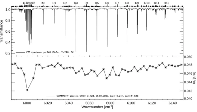
Fig. 1. Example of a recorded FTS methane transmission spectrum at 240.1 hPa (top) and a SCIAMACHY reflectance spectrum over the
Sahara (bottom). On top of the plot, a stick spectrum of methane in logarithmic scale is depicted to indicate line positions and strengths. In addition, the attribution to Q and R-branch transitions in the 2ν3band is given. Please note that the SCIAMACHY spectrum is not absolute-radiometric calibrated, so only relative variations should be considered. The major absorber in the SCIAMACHY spectrum is CH4 but smaller absorptions by CO2and H2O are also present.
about 6000 cm−1 as well as the more widely spaced tran-sitions in the R branch at higher wavenumbers. The spec-tral resolution of SCIAMACHY in this channel is relatively poor with a FWHM (Full width at half maximum) of 1.33 nm (≈4.8 cm−1), sampling the entire Q-branch with a mere 3-4 detector pixels.
Thus, individual lines are not resolved, so that incorrect line-shapes do not necessarily result in systematic retrieval residuals. However, if absorptions are strong, the line-shape and pressure shifts govern the sensitivity of the retrievals with respect to trace gas perturbations (Frankenberg et al., 2005b) as broader lines absorb more efficiently. This can cause systematic biases that change with the degree of satura-tion of the absorpsatura-tion lines, i.e. also with viewing geometry. Washenfelder et al. (2003) already found systematic biases in methane total columns retrieved from ground-based FTIR measurements in the P-branch of the 2ν3band.
For methane, the HITRAN 2004 linelist (Rothman et al., 2005; Brown et al., 2003) in this region is mainly based on empirical line positions and intensities of Margolis (1988, 1990). Measurements were performed at low pressures, thus only estimated broadening coefficients from limited mea-surements were adopted. The widths ranged from 0.054 to 0.066 cm−1atm−1at 296 K for J′′=0 to 10, and transitions of the same lower state energy were given the same widths re-gardless of rotational symmetry (A,F,E). All air-broadened pressure shifts were set to a constant –0.008 cm−1atm−1.
Margolis (1990) originally provided calculated ground state energies for assigned 2ν3 transitions and empirical lower state energies for many of the unassigned features, but in HI-TRAN 2004, all the empirical values were replaced by –1, leaving lower state energies only for the assigned transitions in the 2ν3band.
a discussion on the effect of the temperature dependence of the broadening coefficient). In this study, we neglect those intricacies of methane spectroscopy but follow a pragmatic approach to determine an updated set of effective methane spectroscopic parameters with focus on pressure-broadening. The paper is structured as follows: Sect. 2 describes the experimental setup, followed by a description of the applied inverse method in Sect. 3. Derived spectroscopic parame-ters are presented and discussed in Sect. 4 and the impact on atmospheric retrievals is shown in Sect. 5. Conclusions are drawn in Sect. 6.
2 Experimental setup
Laboratory spectra were recorded over the 5600–6300 cm−1 spectral range with a Bruker IFS 120 HR FTS located at the Institute of Environmental Physics of the University of Bre-men. All spectra were obtained using a tungsten lamp as the infrared source, a 1.7 mm input aperture at the entrance of the FTS, a CaF2 beamsplitter and a liquid nitrogen cooled InSb detector. An optical filter was used to reduce the band-pass. This optical filter was not wedged, which resulted in a sinusoidal structure in the continuum. The gas mixtures were introduced in a 140 cm cell. For thermal stabilization and insulation the cell body is enclosed by 2 coaxial quartz jackets. The inner one is temperature stabilized by a flow of ethanol from a thermostatic bath. The outer one is evacuated for thermal insulation. Windows at the front and back end of the cell are made of CaF2. The cell was located behind the interferometer and the light passed twice through the cell before being detected.
Transmission spectra were calculated by dividing sample spectra (resolution=0.011 cm−1) by the spectra obtained for the evacuated cell (resolution=0.1 cm−1). Twenty-five inter-ferograms were co-added for the calculation of the spectra, resulting in a signal-to-noise of about 200 for the transmis-sion spectra.
To achieve a uniform and constant methane mixing ratio in the cell, it was first filled with N2, then with methane and finally with N2. During the measurements the pressure in the cell remained stable to within 0.6% or better. Table 1 gives an overview of measurement conditions and measured spectra applied in this study. All spectra were recorded consecutively on the same day, and we assumed the internal calibration of the FTS was unchanged during that time. The pressure in the absorption vessel was measured with two independent capac-itive pressure transducers of 500 hPa and 1000 hPa maximum range (MKS Baratron).
3 Data analysis
We applied a nonlinear fitting approach to derive the spec-tral line parameters pressure-broadening coefficient and pressure-induced shift. Parameters for each individual line
were fitted using multiple laboratory spectra simultaneously. Relative line intensities were also fitted but strictly con-strained to the Margolis (1988) values given in HITRAN, permitting only small deviations.
Details about the multispectrum fitting technique and its advantages can be found in Benner et al. (1995). Even though the multispectrum approach greatly reduced uncertainty in the retrieval, the inverse problem remained underdetermined as the blended lines could not be fully separated. For this reason, we added additional constraints using the Optimal Estimation technique (Rodgers, 2000). This approach al-lowed us to attribute prior uncertainties to the target param-eters, thereby minimising oscillations of parameters whose retrieval errors would be strongly correlated in an uncon-strained least squares approach. The solution to this nonlin-ear constrained least squares approach which maximises the a posteriori probability density function of the state vector is given by Rodgers (2000):
xi+1=xa+
KTi S−ǫ1Ki+S−a1
−1
KTi S−ǫ1
·[y−F(xi)+Ki(xi −xa)], (1) where
xa= a priori state vector,
xi =state vector at theith iteration, Sǫ=(pixel)error covariance matrix, Sa=a priori covariance matrix, F(xi)=forward model evaluated atxi,
Ki =Jacobian of the forward model atxi, y=measurement vector.
In our particular case the state vector comprised relative line intensity, pressure broadening parameter and pressure-induced shift of each individual line as well as a low or-der polynomial (for each spectrum separately) to account for broad-band baseline structures. The forward model simu-lates the transmission spectra of the gas cells depending on the integrated column density of methane (fixed, equals con-centrationctimes absorption path lengthl) and the spectral parameters to be retrieved:
Fj(ν)=(a0,j+a1,jν)·fILS(ν)⊗exp −X
i
Si·cj ·l·fvoigt,γi(ν−δi · p
pref
−ν0,i
!
(2) wherefILSis the instrumental line-shape (in our case a sinc convolved with a box function) and⊗denotes convolution.
Table 1.Laboratory measurement conditions for the FTS methane spectra. FTS optical path difference was 90 cm and gas cell length 140 cm, traversed twice for the measurement.
CH4mixing ratio [%] Temperature [K] total pressure at start [hPa] at start of scan increase during scan [%]
≈1.2 295.65 900.0 0.1
≈2 295.65 500.0 0.2
≈2 296.15 239.9 0.2
≈2 297.15 125.7 0.6
Each line is treated separately, even for multiplets, and no cross-correlations between lines is assumed (i.e.Sa is diag-onal). A standard Voigt line-shape is applied and the Ja-cobian of the transmission with respect to shift and broad-ening coefficients computed analytically, as explained in Schreier (1992) and references therein. Self-broadening was neglected since the methane volume mixing ratio in the cell was 2% at most.
From a measurement perspective, no attempt was made to determine an accurate total methane content in the cell a pri-ori. Hence, the integrated column density of methane was determined using a fit covering the isolated R0 and R1 tran-sitions. The line strengths retrieved in this study are thereby linked to the R0 and R1 strengths given in HITRAN (Margo-lis, 1988). For the final determination of spectral parameters, cell column densities were kept fixed. Prior line strengths were taken from HITRAN and prior pressure shifts are all re-set to –0.011 cm−1atm−1as Kapitanov et al. (2007) reports this pressure shift for the R3 triplet.
Prior broadening coefficients were not taken from HI-TRAN but adapted from measurements in the fundamental by Pine (1992, 1997), as done by Washenfelder et al. (2003). The actual fitting was performed in 10 cm−1bins for the sake of computational efficiency. In the inversion, four N2 broad-ened spectra at different pressures at room temperature were used (see Table 1). As we were mainly interested in broaden-ing coefficients, we applied relatively strict prior constraints for line intensity and pressure shift. We then performed retrievals with increasingly stricter constraints on pressure broadening and found that only for prior covariances be-low about(0.002 cm−1atm−1)2, fit residuals started getting worse. Hence we chose this value as optimal constraint on pressure broadening. Depending on the spectral microwin-dow, the fit typically converged within 3–10 iterations. Ta-ble 2 lists the employed prior uncertainties for the individual parameters.
4 Results and discussion
Figures 2, 3 and 4 show the fit results for the P, Q and R-branch, respectively. Only measured FTS spectra and fitting residuals are displayed. As can be seen in the systematic red residuals, applying the HITRAN database yields wrong
line-Table 2.Fit parameters used in the inversion.
prior 1σof
relative line intensity δN2[cm−1atm−1] γN2[cm−1atm−1]
0.1% 0.001 0.002
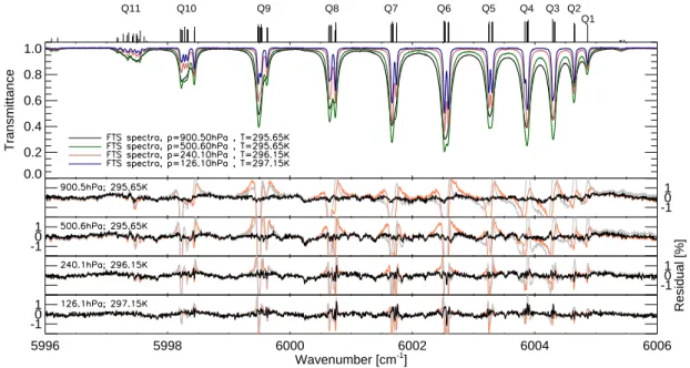
widths and partly shifted lines. While there only seems to be a shift for low rotational levels in the Q branch, higher levels show systematic residuals typical of too high broaden-ing coefficients (wbroaden-ings too strong, line center too weak). The P and R-branches behave similarly and a zoom on the R6 multiplet in Fig. 5 shows the improvements in the fits more clearly. Looking closely at the R6 multiplet, some systematic residuals at intermediate pressures (125 and 250 hPa) exist, hinting at deviations from the Voigt line-shape, perhaps due to Dicke-narrowing. Line-mixing as observed in theν3 fun-damental can also play a role. The same holds true for other transitions. However, those residuals are typically below 1%, being very small compared to residuals induced when apply-ing the current HITRAN broadenapply-ing coefficients. Overall, the final residuals after fitting line parameters show far less systematic features and are dominated by the instrumental artifact of channeling due to the applied spectral filter.
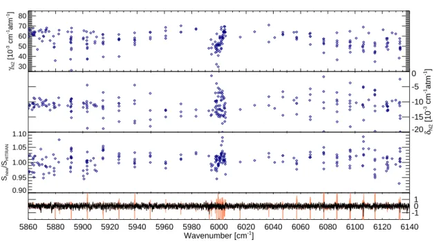
The fitted N2broadening coefficients and pressure shifts for strong transitions in the spectral region under investiga-tion are shown in Fig. 6, along with the ratio of present and HITRAN line strengths. To estimate possible systematic er-rors and the impact of prior values in the retrieved parame-ters, additional fits were performed with varying assumptions as a sensitivity study:
– 2 fits with different low frequency correction terms for the channeling;
– 1 fit where methane abundances in the cell are an addi-tional fit parameter, i.e. not fixed;
– 1 fit with HITRAN broadening and pressure shift pa-rameters as prior;
0.0 0.2 0.4 0.6 0.8 1.0
Transmittance
-1 0 1
-1 0 1
-1 0 1
Residual [%]
5860 5880 5900 5920 5940 5960 5980
Wavenumber [cm-1]
-1 0 1
P1 P2 P3 P4 P5 P6 P7 P8 P9 P10
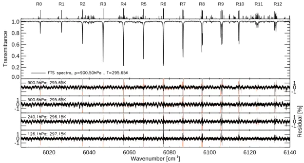
Fig. 2. Fit results of the multi-spectra inversion for the P-branch. The upper panel depicts the N2broadened FTS spectrum at 900.5 hPa.
The lower panels show the fitting residuals for each FTS spectrum (decreasing pressure from top to bottom) separately in black (measured-modelled times 100). The red lines indicate residuals if no changes to the HITRAN database were applied. The gray lines show residuals using the HITRAN database but replacing broadening coefficients with results by Pine (1992, 1997) in the fundamental.
0.0 0.2 0.4 0.6 0.8 1.0
Transmittance
-1 0 1
-1 0 1
-1 0 1
Residual [%]
5996 5998 6000 6002 6004 6006
Wavenumber [cm-1]
-1 0 1
Q11 Q10 Q9 Q8 Q7 Q6 Q5 Q4 Q3 Q2 Q1
Fig. 3.As in Fig. 2 but for the Q-branch and with all FTS spectra plotted in the upper panel (black: 900.5 hPa; green:500.6 hPa; red:240.1 hPa;
blue:126.1 hPa)
Table 3 gives an overview of the results for the transitions of the 2ν3 band that are assigned in HITRAN (please note that some upper state rotational levels are not yet attributed to specific transitions). The outcome of the sensitivity study is used as an error estimate for retrieved broadening coefficients and pressure shifts.
0.0 0.2 0.4 0.6 0.8 1.0
Transmittance
-1 0 1
-1 0 1
-1 0 1
Residual [%]
6020 6040 6060 6080 6100 6120 6140
Wavenumber [cm-1]
-1 0 1
R0 R1 R2 R3 R4 R5 R6 R7 R8 R9 R10 R11 R12
Fig. 4.As in Fig. 2 but for the R-branch.
0.0 0.2 0.4 0.6 0.8 1.0
Transmittance
-2 0 2
-2 0 2
-2 0 2
Residual [%]
6076.0 6076.5 6077.0 6077.5 6078.0 Wavenumber [cm-1]
-2 0 2
Fig. 5.As in Fig. 3 but for the R6 manifold with six strong
transi-tions. The sum of the measured intensities in the manifold is greater by only 1.2% compared to the Margolis (1988) values. In contrast, the average of measured widths is 19% smaller than the average of default widths applied in HITRAN. The residuals seen in the fit of the lowest pressure spectrum could arise from combined inaccura-cies of the retrieved positions, relative strengths, widths, the pres-ence of weak transitions not included in the database or effects of non-Voigt line-shapes.
a systematic dependence on the prior. Figure 7 shows the retrieved broadening parameters as a function of|m|, where
|m|corresponds to the rotational state J (upper state J for R branch lines, lower state for the Q and P-branch). The|m|
dependence is very similar for all branches, slightly increas-ing in the beginnincreas-ing with decreasincreas-ing widths for higher rota-tional levels. As for the comparison with results from theν3 band (Pine, 1992, 1997), which are displayed in the lower panel, we see a slightly different|m|dependence, especially at higher rotational levels our measurements show systemat-ically lower broadening coefficients. Pine (1992, 1997) in-cluded collisional narrowing in their analysis and broaden-ing parameters derived with a non-Voigt profile cannot be easily compared with Voigt-only retrievals, as can be seen in Dufour et al. (2003). However, Predoi-Cross et al. (2006) noted similar differences at higher J in the air-broadened widths at 4300 cm−1. Finally, at the end of the present study, new measurements of N2-broadening in the ν4 fundamen-tal were reported by Martin and Lep`ere (2008). Compari-son for 31 transitions with the same rotational quantum as-signments produced an average ratio (ν4 to 2ν3 widths) of 1.01±13%. Given the experimental precisions of the stud-ies, the large root-mean-square is interpreted as evidence of the vibrational dependences of the widths, as discussed by Predoi-Cross et al. (2006). However, such conclusions must await theoretical validation through the calculations such as those produced by Antony et al. (2008).
30 40 50 60 70 80
γN2
[10
-3 cm -1atm -1]
-20 -15 -10 -5 0
δN2
[10
-3 cm -1atm -1]
0.90 0.95 1.00 1.05 1.10
Snew
/S
HITRAN
5860 5880 5900 5920 5940 5960 5980 6000 6020 6040 6060 6080 6100 6120 6140 Wavenumber [cm-1]
-1 0 1
Fig. 6. N2-broadening coefficients (upper panel, in 10−3cm−1atm−1), pressure shifts (middle panel, in 10−3cm−1atm−1) and ratio
of present line intensities compared to HITRAN (lower panel, mean ratio=1.013) retrieved for all transitions with line intensities above 5·10−23cm−1/(molecule cm−2). The lowest panel again depicts fitting residuals (black line) and residuals assuming HITRAN parameters (red) for the 900 hPa spectra.
in retrieved broadening coefficients within a multiplet should be interpreted with care as many solutions can lead to iden-tical line-shapes. For example, different retrieved pressure shifts within a multiplet might accommodate line-mixing or Dicke narrowing features, thereby not representing the pres-sure shift in its physical sense any more. However, the main objective of this work is to create a set of empirical spectro-scopic parameters that allows a best possible modelling of methane cross sections at typical pressures encountered in the Earth’s atmosphere applying the simple and widely-used Voigt line-shape.
There are only a few studies of broadening parameters in the 2ν3band to compare with and a comparison for multi-plets is not straightforward as the results depend on a va-riety of assumptions that might differ from study to study. However, for the fully isolated R0 and R1 lines a compari-son is possible with work from Darnton and Margolis (1973) and also with the results from Pine (1997) for the fundamen-tal. The comparison is shown in Table 4 and shows very good agreement between the different results, both in abso-lute terms and also concerning the difference of the broaden-ing coefficient between the R0 and R1 line.
4.1 Open issues
Studies of methane pressure broadening are greatly hindered by the lack of basic characterization of the spectrum in this region. The spectral interval between 4800 and 6300 cm−1
contains 14 vibrational bands with some 60 sub-vibrational components. A complete linelist would likely contain more than 20,000 features, but at present no global analysis has been published to provide a reliable calculation of line posi-tions, strengths and lower state energies. Similarly, there is no theoretical model that predicts pressure broadening coeffi-cients with the accuracies required for state-of-the-art remote sensing. Hence, more laboratory measurements and develop-ment of theoretical models are needed to achieve 1% accura-cies for line intensities and broadening parameters as well as to resolve line-mixing and collisional-narrowing effects.
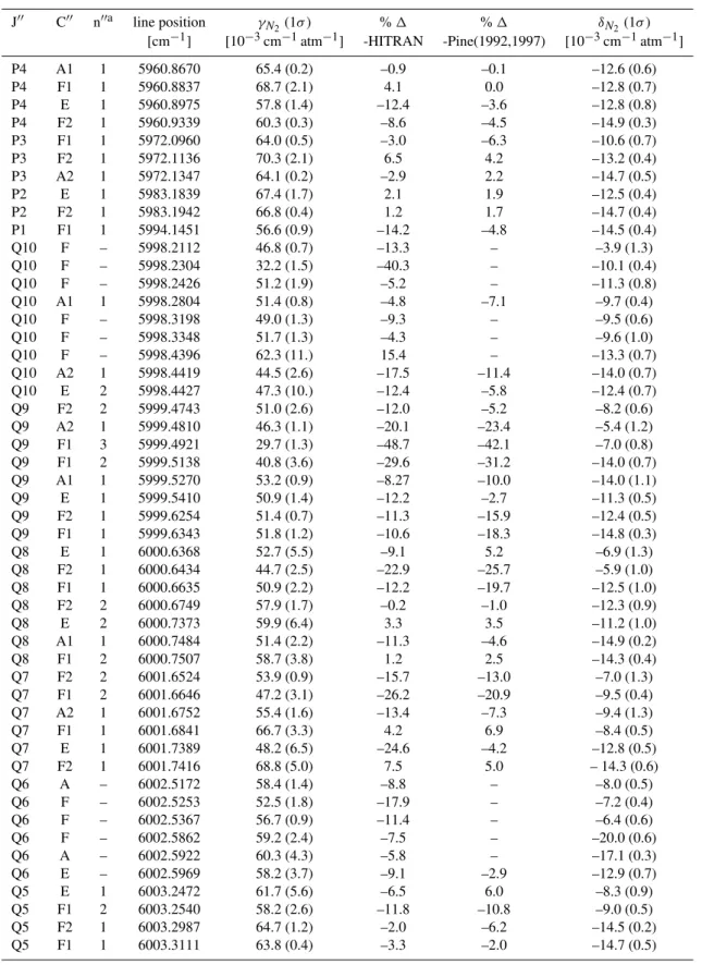
Table 3. Retrieved broadening coefficients and pressure shifts in the 2ν3band for12CH4listed for lower rotational level J′′, symmetry species C′′ and ordering index n′′. For broadening coefficients and pressure shifts, the standard deviation of the fitted parameters in the sensitivity study is provided as error estimate. The differences to HITRAN and to Pine (1992, 1997) values are listed separately, calculated as ((γthis study−γreference)/γreference∗100). Broadening parameters are given for 296 K, assuming a temperature dependence exponent of 0.75. A more detailed list as well as retrieved parameters for all lines are provided in the supplementary material. http://www.atmos-chem-phys. net/8/5061/2008/acp-8-5061-2008-supplement.zip
J′′ C′′ n′′a line position γN2(1σ) %1 %1 δN2(1σ) [cm−1] [10−3cm−1atm−1] -HITRAN -Pine(1992,1997) [10−3cm−1atm−1]
P10 F – 5891.0652 57.2 (8.8) 5.9 – –9.6 (0.3)
P10 A2 1 5891.0676 54.2 (5.7) 0.4 6.1 –9.6 (0.5)
P10 E – 5891.0695 37.2 (10.) –31.1 – –11.7 (1.0)
P10 F – 5891.3418 53.4 (1.1) –1.1 – –10.0 (0.7)
P10 F – 5891.3784 56.1 (1.3) 3.9 – –11.4 (0.8)
P10 A1 1 5891.4572 58.0 (0.5) 7.4 3.3 –13.2 (0.3)
P10 F – 5891.5008 59.4 (1.5) 10.0 – –9.1 (0.9)
P10 F1 1 5891.5826 46.7 (1.6) –13.5 –17.9 –8.9 (1.2) P10 E 1 5891.6159 26.2 (1.8) –51.4 –27.5 –13.0 (0.6) P10 F2 1 5891.6452 48.1 (1.5) –10.9 –15.6 –15.2 (0.7)
P9 F – 5902.9488 52.1 (0.6) –10.1 – –9.8 (0.5)
P9 F – 5902.9645 55.7 (0.9) –4.0 – –10.9 (0.5)
P9 F – 5903.1035 59.5 (3.3) 2.6 – –11.2 (1.1)
P9 E – 5903.1591 52.3 (1.1) –9.8 – –11.5 (0.7)
P9 F – 5903.1800 58.9 (1.1) 1.6 – –12.1 (0.6)
P9 A1 1 5903.2861 47.7 (0.4) –17.7 –15.9 –4.4 (0.4)
P9 F – 5903.3376 37.2 (1.0) –35.8 – –13.2 (1.0)
P9 F – 5903.3654 37.6 (1.9) –35.1 – –22.9 (0.5)
P9 A2 1 5903.3857 49.0 (0.6) –15.5 –14.5 –18.7 (1.0)
P8 A1 1 5914.7515 53.3 (1.1) –8.1 0.2 –9.5 (0.7)
P8 F1 2 5914.7651 61.9 (5.0) 6.7 7.9 –11.4 (0.5)
P8 E 2 5914.7762 61.5 (1.9) 6.0 9.8 –11.8 (0.9)
P8 F2 2 5914.9181 58.2 (0.6) 0.3 –1.0 –12.2 (0.3)
P8 F1 1 5915.0006 52.2 (0.5) –10.0 –15.4 –6.8 (0.4) P8 E 1 5915.0461 39.5 (0.9) –31.8 –18.2 –18.8 (0.4) P8 F2 1 5915.0631 54.5 (0.6) –6.0 –8.2 –15.3 (0.5) P7 F2 1 5926.4662 56.5 (0.3) –11.7 –11.2 –10.4 (0.4)
P7 F1 1 5926.4837 61.7 (0.9) –3.6 2.2 –8.5 (0.3)
P7 A2 1 5926.5755 57.6 (0.2) –10.0 –2.8 –12.9 (0.2) P7 F2 2 5926.6250 56.4 (0.6) –11.8 –8.4 –10.5 (0.8) P7 E 1 5926.6482 39.9 (1.1) –37.6 –16.2 –11.4 (0.4) P7 F1 2 5926.6785 57.0 (0.4) –10.9 –3.7 –16.5 (0.3) P6 E 1 5938.0571 56.7 (0.8) –11.4 –6.9 –10.6 (0.4) P6 F2 2 5938.0661 63.3 (1.1) –1.1 –1.6 –9.5 (0.2) P6 A2 1 5938.0947 58.3 (0.3) –8.9 –4.9 –4.4 (0.2) P6 F2 1 5938.1676 53.5 (0.4) –16.4 –18.8 –16.9 (0.6) P6 F1 1 5938.1901 51.5 (1.1) –19.5 –18.6 –21.3 (0.3) P6 A1 1 5938.2086 55.7 (0.1) –12.9 –6.5 –16.3 (0.5)
P5 F1 1 5949.5276 64.1 (0.2) –2.9 2.9 –12.8 (0.4)
P5 F2 1 5949.5526 63.6 (0.6) –3.6 –5.0 –7.1 (0.2) P5 F1 2 5949.6100 57.2 (0.9) –13.3 –11.6 –18.0 (0.3)
P5 E 1 5949.6214 59.0 (0.9) –10.6 3.1 –15.8 (0.5)
Table 3.Continued.
J′′ C′′ n′′a line position γN2(1σ) %1 %1 δN2(1σ) [cm−1] [10−3cm−1atm−1] -HITRAN -Pine(1992,1997) [10−3cm−1atm−1]
P4 A1 1 5960.8670 65.4 (0.2) –0.9 –0.1 –12.6 (0.6)
P4 F1 1 5960.8837 68.7 (2.1) 4.1 0.0 –12.8 (0.7)
P4 E 1 5960.8975 57.8 (1.4) –12.4 –3.6 –12.8 (0.8) P4 F2 1 5960.9339 60.3 (0.3) –8.6 –4.5 –14.9 (0.3) P3 F1 1 5972.0960 64.0 (0.5) –3.0 –6.3 –10.6 (0.7)
P3 F2 1 5972.1136 70.3 (2.1) 6.5 4.2 –13.2 (0.4)
P3 A2 1 5972.1347 64.1 (0.2) –2.9 2.2 –14.7 (0.5)
P2 E 1 5983.1839 67.4 (1.7) 2.1 1.9 –12.5 (0.4)
P2 F2 1 5983.1942 66.8 (0.4) 1.2 1.7 –14.7 (0.4)
P1 F1 1 5994.1451 56.6 (0.9) –14.2 –4.8 –14.5 (0.4)
Q10 F – 5998.2112 46.8 (0.7) –13.3 – –3.9 (1.3)
Q10 F – 5998.2304 32.2 (1.5) –40.3 – –10.1 (0.4)
Q10 F – 5998.2426 51.2 (1.9) –5.2 – –11.3 (0.8)
Q10 A1 1 5998.2804 51.4 (0.8) –4.8 –7.1 –9.7 (0.4)
Q10 F – 5998.3198 49.0 (1.3) –9.3 – –9.5 (0.6)
Q10 F – 5998.3348 51.7 (1.3) –4.3 – –9.6 (1.0)
Q10 F – 5998.4396 62.3 (11.) 15.4 – –13.3 (0.7)
Q10 A2 1 5998.4419 44.5 (2.6) –17.5 –11.4 –14.0 (0.7) Q10 E 2 5998.4427 47.3 (10.) –12.4 –5.8 –12.4 (0.7) Q9 F2 2 5999.4743 51.0 (2.6) –12.0 –5.2 –8.2 (0.6) Q9 A2 1 5999.4810 46.3 (1.1) –20.1 –23.4 –5.4 (1.2) Q9 F1 3 5999.4921 29.7 (1.3) –48.7 –42.1 –7.0 (0.8) Q9 F1 2 5999.5138 40.8 (3.6) –29.6 –31.2 –14.0 (0.7) Q9 A1 1 5999.5270 53.2 (0.9) –8.27 –10.0 –14.0 (1.1) Q9 E 1 5999.5410 50.9 (1.4) –12.2 –2.7 –11.3 (0.5) Q9 F2 1 5999.6254 51.4 (0.7) –11.3 –15.9 –12.4 (0.5) Q9 F1 1 5999.6343 51.8 (1.2) –10.6 –18.3 –14.8 (0.3)
Q8 E 1 6000.6368 52.7 (5.5) –9.1 5.2 –6.9 (1.3)
Q8 F2 1 6000.6434 44.7 (2.5) –22.9 –25.7 –5.9 (1.0) Q8 F1 1 6000.6635 50.9 (2.2) –12.2 –19.7 –12.5 (1.0) Q8 F2 2 6000.6749 57.9 (1.7) –0.2 –1.0 –12.3 (0.9)
Q8 E 2 6000.7373 59.9 (6.4) 3.3 3.5 –11.2 (1.0)
Q8 A1 1 6000.7484 51.4 (2.2) –11.3 –4.6 –14.9 (0.2)
Q8 F1 2 6000.7507 58.7 (3.8) 1.2 2.5 –14.3 (0.4)
Q7 F2 2 6001.6524 53.9 (0.9) –15.7 –13.0 –7.0 (1.3) Q7 F1 2 6001.6646 47.2 (3.1) –26.2 –20.9 –9.5 (0.4) Q7 A2 1 6001.6752 55.4 (1.6) –13.4 –7.3 –9.4 (1.3)
Q7 F1 1 6001.6841 66.7 (3.3) 4.2 6.9 –8.4 (0.5)
Q7 E 1 6001.7389 48.2 (6.5) –24.6 –4.2 –12.8 (0.5)
Q7 F2 1 6001.7416 68.8 (5.0) 7.5 5.0 – 14.3 (0.6)
Q6 A – 6002.5172 58.4 (1.4) –8.8 – –8.0 (0.5)
Q6 F – 6002.5253 52.5 (1.8) –17.9 – –7.2 (0.4)
Q6 F – 6002.5367 56.7 (0.9) –11.4 – –6.4 (0.6)
Q6 F – 6002.5862 59.2 (2.4) –7.5 – –20.0 (0.6)
Q6 A – 6002.5922 60.3 (4.3) –5.8 – –17.1 (0.3)
Q6 E – 6002.5969 58.2 (3.7) –9.1 –2.9 –12.9 (0.7)
Q5 E 1 6003.2472 61.7 (5.6) –6.5 6.0 –8.3 (0.9)
Table 3.Continued.
J′′ C′′ n′′a line position γN2(1σ) %1 %1 δN2(1σ) [cm−1] [10−3cm−1atm−1] -HITRAN -Pine(1992,1997) [10−3cm−1atm−1]
Q4 F2 1 6003.8370 64.0 (0.1) –3.0 –2.9 –8.7 (0.2) Q4 F1 1 6003.8714 64.3 (1.7) –2.6 –5.8 –11.5 (0.7)
Q4 E 1 6003.8830 65.1 (4.8) –1.4 5.8 –11.0 (0.3)
Q4 A1 1 6003.8928 69.6 (1.7) 5.5 4.3 –12.0 (0.7)
Q3 A2 1 6004.2930 66.6 (0.2) 0.9 4.1 –12.1 (0.4)
Q3 F1 1 6004.3133 69.5 (1.7) 5.3 0.0 –14.1 (0.3)
Q3 F2 1 6004.3291 63.9 (0.5) –3.2 –0.1 –16.4 (0.6) Q2 F2 1 6004.6435 63.8 (0.4) –3.3 –2.4 –10.4 (0.2)
Q2 E 1 6004.6527 64.1 (0.8) –2.9 1.4 –13.3 (0.2)
Q1 F1 1 6004.8632 60.2 (0.3) –8.8 –5.5 –15.2 (0.1) R0 A1 1 6015.6643 59.1 (0.1) –10.4 0.9 –12.5 (0.2) R1 F1 1 6026.2274 64.4 (0.2) –2.4 –0.1 –11.1 (0.0) R2 E 1 6036.6536 54.2 (2.3) –17.8 –7.9 –8.2 (0.2)
R2 F2 1 6036.6584 71.0 (1.9) 7.6 6.2 –11.1 (0.2)
R3 F2 1 6046.9420 62.1 (2.1) –5.9 –6.3 –6.6 (0.5) R3 F1 1 6046.9527 63.9 (3.6) –3.2 –5.5 –8.4 (0.1) R3 A2 1 6046.9647 61.3 (1.7) –7.1 3.1 –14.4 (0.2)
R4 E 1 6057.0778 59.0 (1.5) –10.6 7.8 –8.6 (0.3)
R4 A1 1 6057.0861 64.2 (2.0) –2.7 7.4 –10.4 (0.5) R4 F1 1 6057.0998 58.1 (1.5) –11.9 –13.9 –10.5 (0.5) R4 F2 1 6057.1273 56.8 (0.2) –13.9 –9.2 –14.1 (0.3) R5 F2 1 6067.0816 59.7 (0.2) –9.5 –7.2 –7.5 (0.1)
R5 F1 1 6067.0997 63.0 (0.4) –4.5 1.4 –5.6 (0.1)
R5 E 1 6067.1485 51.8 (0.6) –21.5 –4.3 –14.8 (0.1) R5 F1 2 6067.1570 59.7 (0.3) –9.5 –1.6 –15.8 (0.2) R6 E 1 6076.9280 53.3 (0.9) –16.7 –4.4 –10.1 (0.3) R6 F2 2 6076.9350 57.2 (0.6) –10.6 –8.1 –6.5 (0.0) R6 A2 1 6076.9540 57.4 (0.2) –10.3 –0.1 –1.7 (0.1) R6 F1 1 6077.0283 55.3 (0.7) –13.5 –10.5 –19.8 (0.5) R6 F2 1 6077.0466 43.5 (0.9) –32.0 –31.6 –21.9 (0.2) R6 A1 1 6077.0636 52.3 (0.1) –18.2 –11.1 –12.1 (0.3) R7 F1 1 6086.6229 50.1 (0.3) –21.7 –16.4 –6.9 (0.2)
R7 F2 1 6086.6350 63.4 (0.6) –0.9 0.9 –9.3 (0.1)
R7 A2 1 6086.7454 53.7 (0.1) –16.0 –0.0 –13.2 (0.1) R7 F2 2 6086.7797 55.5 (0.5) –13.2 –6.0 –9.8 (0.5) R7 E 1 6086.7994 36.6 (0.7) –42.8 –15.4 –10.7 (0.1) R7 F1 2 6086.8307 51.5 (0.2) –19.5 –6.7 –16.5 (0.2) R8 F1 2 6096.1665 48.1 (1.2) –17.0 –17.0 –7.6 (0.3) R8 A1 1 6096.1743 50.0 (1.9) –13.7 2.6 –12.5 (0.7) R8 E 2 6096.1809 64.8 (5.6) 11.7 21.1 –10.4 (0.6) R8 F2 2 6096.3727 55.6 (0.1) –4.1 0.7 –11.5 (0.1) R8 F1 1 6096.4244 54.2 (0.1) –6.6 –7.6 –3.7 (0.2) R8 E 1 6096.4856 44.1 (0.5) –23.9 –7.8 –21.5 (0.3) R8 F2 1 6096.5015 50.8 (0.3) –12.4 –14.5 –18.1 (0.2) R9 F1 1 6105.6259 50.2 (4.4) –13.4 –13.2 –10.8 (0.6) R9 F2 1 6105.6261 49.2 (5.6) –15.1 –14.0 –11.1 (0.9)
R9 F – 6106.0402 46.2 (1.1) –20.3 – –5.2 (0.4)
R9 A1 1 6106.0505 69.0 (1.1) 19.0 28.5 –4.9 (0.2)
R9 E – 6106.1943 52.7 (7.7) –9.1 – –17.1 (1.4)
Table 4.Comparison of retrieved R0 and R1 N2-broadening coefficients with literature.
line This study Darnton and Margolis (1973) Pine (1997) (ν3)
R0 59.1 (±0.2(2σ )) 59.0 (±06.7(1σ )) 58.7 (±0.17(1σ )) R1 64.4 (±0.4(2σ )) 63.7 (±10.2(1σ )) 64.7 (±0.08(1σ ))
4.2 Additional information
Along with the results described in the paper, we provide two files with supplementary informa-tion http://www.atmos-chem-phys.net/8/5061/2008/ acp-8-5061-2008-supplement.zip. One file lists retrieval results (line strengths, broadening coefficients and pressure induced shifts) and associated standard deviations from the sensitivity studies for about 1300 lines in the 5860 to 6184.5 cm−1range. A second file provides these results in a HITRAN-format (2001) file for easy application. In this file, the following changes were made:
– retrieved N2-broadening coefficients are scaled with 0.985 to give an estimate of air-broadening;
– empirical lower state energies measured by Margolis (1990) are restored;
– exponent of the temperature dependence of broadening has been reset to 0.85 for all lines;
– default value for shifts are changed from –0.008 to – 0.011 cm−1atm−1at 296 K.
Even though the results of this study are most re-liable for almost 150 strong lines of the 2ν3 band, about 1300 transitions in the considered spectral range have been fitted and the results incorporated in the sup-plementary files http://www.atmos-chem-phys.net/8/5061/ 2008/acp-8-5061-2008-supplement.zip.
5 Impact on atmospheric methane measurements
Erroneous broadening coefficients can have a profound im-pact on the retrieval of gases (Washenfelder et al., 2003). Mondelain et al. (2007) found deviations of up to 7% due to line-mixing and pressure broadening effects in atmospheric profile retrievals. In this study we consider total column re-trievals which should be less susceptible to errors in line-shapes as compared to profile retrievals that actually rely on an accurate knowledge of the line-shape to differentiate trace gas perturbations at different height layers. However, possi-ble errors depend on a variety of factors like spectral resolu-tion, retrieval method and viewing geometry.
Here we discuss two kinds of measurements, first a high resolution ground based direct sun measurement using an FTIR instrument located in Bremen, Germany, and second
30 40 50 60 70 80
γN2
[10
-3 cm -1atm -1]
1 2 3 4 5 6 7 8 9 10
|m| 0.6
0.8 1.0 1.2 1.4
This work / Pine(1992,1997)
Fig. 7. Measured N2-broadening coefficients retrieved in the P, Q
and R-branch (depicted as black square, red triangle, blue diamond, respectively) as a function of|m|, where|m|is the lower state J for P and Q transitions and the upper state J for R branch lines. For easier identification, branches are slightly shifted with respect to|m|. The lower panels depicts the ratio of the retrievals with results from Pine (1992, 1997) in theν3band. Values greater than one indicate that broadening coefficients retrieved in this study are larger than those from Pine (1992, 1997)
retrievals from the SCIAMACHY instrument (Bovensmann et al., 1997) onboard the European research satellite EN-VISAT. As SCIAMACHY retrievals are the main driver for this study, we focus only on the Q and R-branch in both cases.
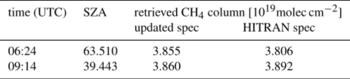
Table 5. FTIR methane total columns retrieved with the updated spectroscopy and HITRAN at two different solar zenith angles. The root mean square of the fit is about 0.5% using HITRAN and im-proves to about 0.3% using the updated spectroscopy.
time (UTC) SZA retrieved CH4column [1019molec cm−2]
updated spec HITRAN spec
06:24 63.510 3.855 3.806
09:14 39.443 3.860 3.892
5.1 Ground based high resolution solar absorption mea-surements
Two ground-based solar absorption FTIR-spectra, covering the near infrared spectral region are analysed. The FTIR measurements were performed at the University of Bre-men (53.1◦N, 8.9◦E) with a Bruker 125 HR and an optical path difference of 45 cm, corresponding to a resolution of 0.022 cm−1. As a possible retrieval bias due to erroneous broadening coefficients largely depends on the observed air-mass (defined as 1/cos(SZA), whereSZAdenotes the so-lar zenith angle), we analyse two spectra from 3 July 2006 at different solar zenith angles, 63.510◦ (Airmass=2.242, 06:24 UTC) and 39.443◦(Airmass=1.295, 09:14 UTC). A fit at high solar zenith angle is shown in Fig. 8. Pressure, tem-perature and water vapour profiles were taken from NCEP (National Centers for Environmental Prediction), the initial CH4 profile from a TM5 model run (similar to the S1 sce-nario described in Bergamaschi et al., 2007) and the CO2 profile set to a constant 380 ppm (parts per million). We used a least squares approach and scaled the entire initial profiles with factors for the respective trace gases. A disk center solar spectrum was calculated from a linelist provided by Geoffrey Toon, Jet Propulsion Laboratory, Pasadena, USA. CO2 spec-troscopic parameters from a recent study by Toth et al. (2007) are applied.
The lower panel in Fig. 8 shows the residuals using the methane spectroscopic parameters derived in this study and the parameters given by HITRAN. It is striking that the new methane spectroscopy largely reduces systematic residual structures, not only for the methane lines itself but also for the CO2 lines which exhibit a slight shift when HITRAN methane spectroscopy is applied. This is most likely due to the updated pressure shifts. Table 5 shows the retrieval results for the two different FTIR spectra applying updated and HITRAN methane spectroscopic parameters. As the time difference between the measurements was short (below 3 hours), the methane vertical column is expected to remain rather constant. This is true for the retrievals using the up-dated spectroscopy, where the difference between the two measurements is only 0.13%, underlining the precision that can be achieved in this spectral range. However, applying HITRAN spectroscopic parameters, the difference is 2.3%,
rendering the retrievals virtually useless for the detection of small changes in atmospheric methane abundances. A simi-lar systematic error depending on sosimi-lar zenith angle was al-ready found by Washenfelder et al. (2003) for the P-branch of the 2ν3band.
5.2 Low resolution space borne measurements by SCIA-MACHY onboard ENVISAT
Previous studies suggest systematic biases in the SCIA-MACHY methane retrievals (Frankenberg et al., 2006; Bergamaschi et al., 2007). Here we analyse the impact of the new spectroscopy using the retrieval approach described in Frankenberg et al. (2005b) for the year 2004. Two re-trieval runs were performed that only differed in methane spectroscopy, all other retrieval parameters being identical. Figure 9 shows the average differences for the entire globe averaged through a year as well as latitudinal averages for individual months. The new retrieval gives in general higher methane columns, ranging from 0 to 1.5%. This can be eas-ily explained by narrower lines that absorb less efficient as they are not resolved by SCIAMACHY (in contrast to the FTIR retrievals). Over highly elevated regions, such as the Himalayas or Andes, the differences are negligible. This can be explained by two reasons: First, the atmosphere is opti-cally thinner, leading to less saturation effects that would be governed by line-widths. Second, pressure broadening and shift are less dominant.
The differences for North America, for example, over the Rocky Mountains are smaller compared to the eastern re-gions. In that particular case, wrong spectroscopic param-eters would create an artificial east-west gradient. The right panel of Fig. 9 depicts the dependence of the mean latitudinal bias on season, exemplified by 4 different months. Differ-ences are minimal in tropical regions where the solar zenith angle is low. However, at higher latitudes the solar zenith angle and thus the bias changes during the year. Artificial seasonal structures with a peak-to-peak amplitude of about 1% could thereby be generated, which is crucial for source inversions as it cannot easily be discerned from seasonally varying methane source.
0.0 0.2 0.4 0.6 0.8 1.0
Transmittance
6000 6020 6040 6060 6080 6100 6120
Wavenumber [cm-1]
-6 -4 -2 0 2 4 6
Residual [%]
Fig. 8.Spectral fit of a ground based FTIR measurement in Bremen, Germany, measured with 45 cm optical path difference at 63.51◦SZA on
3 July 2006. The upper panel shows the spectrum and the contributions of the individual gases as well as the sun (black: measured spectrum; red: Methane; green: Carbon dioxide; blue: Water vapor; grey: sun). The lower panel depicts the fit residuals (Measured-modelled) using the spectroscopic parameters from this study (black) and HITRAN(red).
0.0 0.5 1.0 1.5 0.0 0.5 1.0 1.5
-80 -60 -40 -20 0 20 40 60 80
2004 Average Individual months
Difference New-HITRAN [%]
Fig. 9. Impact of spectroscopy on methane retrievals by SCIAMACHY onboard ENVISAT. The left panel shows the percentage
differ-ences averaged over the year 2004 ((xVMR CH4(New spectroscopy) – CH4xVMR(HITRAN spectroscopy))/CH4xVMR(HITRAN spec-troscopy)*100) on a 1 by 1 degree grid. The right panel shows the mean latitudinal differences for individual months (x-axis as in left panel; y-axis: in degree latitude).
(about 0.3%) while Frankenberg et al. (2006) found system-atic seasonal biases of about 40 ppb peak to peak. Most of this previous bias is actually caused by spectroscopic inter-ferences with water vapor, as shown by Frankenberg et al. (2008). These findings are already taken into account in this study, eliminating a large part of the seasonal bias. Using the old retrieval version (HITRAN methane spectroscopic parameters, scaled by 1.02), however, still shows a distinct deviation by about 10 ppb from April through September, corresponding with high air mass factors.
6 Conclusions
01Feb 01Mar 01Apr 01May 01Jun 01Jul 01Aug 01Sep 01Oct 01Nov 01Dec 2004
1695 1700 1705 1710 1715 1720
CH
4
xVMR [ppbv]
2.0 2.2 2.4 2.6 2.8 3.0 3.2
Air Mass Factor
Fig. 10.Timeseries of SCIAMACHY methane column averaged mixing ratios over Australia in 2004. Concurrent CO2retrievals have been
used as proxy for the light path (Frankenberg et al., 2005a, 2006), using CarbonTracker by NOAA for model CO2profiles to minimise the impact of CO2variations. The air mass factor is shown in grey and a decontamination period (±10 days) of the satellite is overlaid as grey box. Time series data have been smoothed with a 30-day running time-average (box filter) and spatially averaged over the entire australian continent between –20 and –30 degree latitude. Black: retrieval with new CH4spectroscopic parameters (this study); red: retrieval with HITRAN CH4spectroscopic parameters; green: modelled CH4mixing ratio.
Compared to the HITRAN spectroscopic database, we found systematically lower broadening parameters, espe-cially at higher rotational levels. These results were con-firmed using ground based solar absorption FTIR measure-ments where we found systematic residuals and biases de-pending on solar zenith angle when applying HITRAN spec-troscopic parameters. The results of this study largely re-duced residuals and the bias. Some small systematic incon-sistencies between modelled and measured methane spec-tra still exist, probably owing to line-mixing and Dicke-narrowing effects. However, compared to the improvements achieved in this study, deviations from the Voigt line-shape are small.
We further show that SCIAMACHY retrievals based on the spectroscopy derived in this work are systematically dif-ferent from a retrieval version using the HITRAN database. Differences for monthly and yearly averages are between 0 and 1.5%, depending on solar zenith angle and surface el-evation. Thus, artificial seasonal structures with a peak-to-peak amplitude of about 1% can be introduced in our par-ticular retrieval setup. With the new spectroscopy, we find only very small differences (max. 5 ppb) as compared to an atmospheric model over Australia for monthly averages.
The main purpose of this study was to provide an effective set of spectroscopic parameters for methane retrievals in the Earth’s atmosphere, minimising systematic seasonal and lati-tudinal biases. The new spectroscopy will not only be helpful for ground-based FTIR and SCIAMACHY retrievals but also be for future space missions such as the GOSAT (Greenhouse gases Observing Satellite) mission by the Japan Aerospace Exploration Agency covering a similar spectral range for re-trieval.
Acknowledgements. CF is supported by the Dutch science
foundation (NWO) through a VENI grant. We acknowledge John Burrows, PI of the SCIAMACHY instrument, for having
initiated the SCIAMACHY project. The experimental data for the study of the broadening parameters, used in this study, was recorded in the Molecular Spectroscopy laboratory of the Institute of Environmental Physics and Remote Sensing of the University of Bremen. This laboratory is funded by the University of Bremen and the German Aerosopsace (DLR) to undertake spectroscopic studies in support of SCIAMACHY science. We thank R. Washenfelder for providing a spectroscopic linelist based on the results of Pine et al. The Netherlands SCIAMACHY Data Center and ESA is greatly acknowledged for providing data and R. van Hees for having written the versatile NADC tools software package. We thank Jan Fokke Merink and Peter Bergamaschi for providing TM5-4DVAR methane model fields and Wouter Peters for providing CarbonTracker results. We also thank A. Segers, C. Schrijvers, and O. Tuinder for providing the ECMWF data. Part of the research described in this paper was performed at the Jet Propulsion Laboratory, California Institute of Technology, under contract with the National Aeronautics and Space Administration (NASA). We acknowledge the European Commission for sup-porting the 6th Framework Programme project HYMN (contract number 037048) and GEOMON (contract number 036677). We further acknowledge exchange of information within the EU 6th FP Network of Excellence ACCENT.
Edited by: W. Lahoz
References
Antony, B. K., Niles, D. L., Wroblewski, S. B., Humphrey, C. M., Gabard, T., and Gamache, R. R.: N2, O2and air-broadened half-widths and line shifts for transitions in theν3band of methane in the 2726–3200 cm−1 spectral region, Journal of Molecular Spectroscopy, 251, 268–281, 2008.
M., et al.: Satellite chartography of atmospheric methane from SCIAMACHY on board ENVISAT: 2. Evaluation based on in-verse model simulations, J. Geophys. Res., 112, D02304, doi: 10.1029/2006JD007268, 2007.
Bovensmann, H., Burrows, J. P., Buchwitz, M., Frerick, J., No¨el, S., Rozanov, V. V., Chance, K. V., and Goede, A. P. H.: SCIA-MACHY: Mission Objectives and Measurement Modes, J. At-mos. Sci., 56, 127–150, 1997.
Brown, L. R., Benner, D. C., Champion, J. P., Devi, V. M., Fejard, L., Gamache, R. R., Gabard, T., Hilico, J. C., Lavorel, B., Loete, M., et al.: Methane line parameters in HITRAN, J. Quant. Spec-trosc. Radiat. Transfer, 82, 219–238, 2003.
Buchwitz, M., de Beek, R., No¨el, S., Burrows, J. P., Bovensmann, H., Schneising, O., Khlystova, I., Bruns, M., Bremer, H., Berga-maschi, P., K¨orner, S., and Heimann, M.: Atmospheric carbon gases retrieved from SCIAMACHY by WFM-DOAS: version 0.5 CO and CH4and impact of calibration improvements on CO2 retrieval, Atmos. Chem. Phys., 6, 2727–2751, 2006,
http://www.atmos-chem-phys.net/6/2727/2006/.
Darnton, L. and Margolis, J. S.: The temperature dependence of the half widths of some self-and foreign-gas-broadened lines of methane., J. Quant. Spectrosc. Radiat. Transfer, 13, 969–976, 1973.
Dufour, G., Hurtmans, D., Henry, A., Valentin, A., and Lep`ere, M.: Line profile study from diode laser spectroscopy in the12CH4 2ν3band perturbed by N2, O2, Ar, and He, J. Mol. Spectrosc., 221, 80–92, 2003.
Frankenberg, C., Meirink, J. F., van Weele, M., Platt, U., and Wagner, T.: Assessing Methane Emissions from Global Space-Borne Observations, Science, 308, 1010–1014, doi:10. 1126/science.1106644, http://www.sciencemag.org/cgi/content/ abstract/308/5724/1010, 2005a.
Frankenberg, C., Platt, U., and Wagner, T.: Iterative maximum a posteriori (IMAP)-DOAS for retrieval of strongly absorbing trace gases: Model studies for CH4and CO2retrieval from near infrared spectra of SCIAMACHY onboard ENVISAT, Atmos. Chem. Phys., 5, 9–22, 2005b.
Frankenberg, C., Meirink, J. F., Bergamaschi, P., Goede, A. P. H., Heimann, M., K¨orner, S., Platt, U., van Weele, M., and Wagner, T.: Satellite chartography of atmospheric methane from SCIAMACHY on board ENVISAT: Analysis of the years 2003 and 2004, J. Geophys. Res., 111, D07303, doi:10.1029/ 2005JD006235, 2006.
Frankenberg, C., Bergamaschi, P., Butz, A., Houweling, S., Meirink, J. F., Petersen, K., Schrijver, H., Warneke, T., and Aben, I.: Tropical methane emissions: A revised view from SCIA-MACHY onboard ENVISAT, Geophys. Res. Lett., 35, L15811, doi:10.1029/2008GL034300, 2008.
Gharavi, M. and Buckley, S. G.: Diode laser absorption spec-troscopy measurement of linestrengths and pressure broadening coefficients of the methane 2ν3band at elevated temperatures, J. Mol. Spectrosc., 229, 78–88, 2005.
IPCC: Climate Change 2007 – The Physical Science Basis: Work-ing Group I Contribution to the Fourth Assessment Report of the IPCC (Climate Change 2007), Cambridge University Press, Cambridge, United Kingdom and New York, NY, USA, 2007. Kapitanov, V. A., Ponomarev, Y. N., Tyryshkin, I. S., and Rostov,
A. P.: Two-channel opto-acoustic diode laser spectrometer and fine structure of methane absorption spectra in 6070–6180 cm−1
region, Spectrochim. Acta A, 66, 811–818, 2007.
Margolis, J. S.: Measured line positions and strengths of methane between 5500 and 6180 cm−1, Appl. Opt., 27, 4038–4051, 1988. Margolis, J. S.: Empirical values of the ground state energies for methane transitions between 5500 and 6150 cm−1, Appl. Opt., 29, 2295–2302, 1990.
Martin, B. and Lep`ere, M.: N2-broadening coefficients in theν4 band of12CH4at room temperature, Journal of Molecular Spec-troscopy, 250, 70–74, doi:10.1016/j.jms.2008.05.001, 2008. Mondelain, D., Payan, S., Deng, W., Camy-Peyret, C., Hurtmans,
D., and Mantz, A. W.: Measurement of the temperature depen-dence of line mixing and pressure broadening parameters be-tween 296 and 90K in theν3band of12CH4and their influence on atmospheric methane retrievals, J. Mol. Spectrosc., 244, 130– 137, 2007.
Mondelain, D., Camy-Peyret, C., Deng, W., Payan, S., and Mantz, A. W.: Study of molecular line parameters down to very low temperature, Appl. Phys. B, 90, 227–233, doi:10.1007/ s00340-007-2918-x, 2008.
Pine, A. S.: Self-, N2, O2, H2, Ar, and He broadening in the ν3 band Q branch of CH4, J. Chem. Phys., 97, 773–785, 1992. Pine, A. S.: N2 and Ar broadening and line mixing in the P and
R branches of theν3band of CH4, J. Quant. Spectrosc. Radiat. Transfer, 57, 157–176, 1997.
Pine, A. S. and Gabard, T.: Multispectrum fits for line mixing in the ν3band Q branch of methane, J. Mol. Spectrosc., 217, 105–114, 2003.
Predoi-Cross, A., Brawley-Tremblay, M., Brown, L. R., Malathy Devi, V., and Benner, D. C.: Multispectrum analysis of 12CH
4from 4100 to 4635 cm−1: II. Air-broadening coefficients (widths and shifts), J. Mol. Spectrosc., 236, 201–215, 2006. Predoi-Cross, A., Unni, A. V., Heung, H., Malathy Devi, V., Benner,
C. D., and Brown, L. R.: Line mixing effects in theν2+ν3band of methane, J. Mol. Spectrosc., 246, 65–76, 2007.
Rodgers, C. D.: Inverse Methods for Atmospheric Sounding, World Scientific, London, 2000.
Rothman, L. S., Jacquemart, D., Barbe, A., Benner, D. C., Birk, M., Brown, L. R., Carleer, M. R., Chackerian, C., Chance, K., Coudert, L. H., et al.: The HITRAN 2004 molecular spectro-scopic database, J. Quant. Spectrosc. Radiat. Transfer, 96, 139– 204, 2005.
Schneising, O., Buchwitz, M., Burrows, J. P., Bovensmann, H., Bergamaschi, P., and Peters, W.: Three years of greenhouse gas column-averaged dry air mole fractions retrieved from satellite – Part 2: Methane, Atmos. Chem. Phys. Discuss., 8, 8273–8326, 2008,
http://www.atmos-chem-phys-discuss.net/8/8273/2008/. Schreier, F.: The Voigt and complex error function – A comparison
of computational methods, J. Quant. Spectrosc. Radiat. Transfer, 48, 743–762, 1992.
Toth, R. A., Brown, L. R., Miller, C. E., Devi, V. M., and Benner, D. C.: Spectroscopic database of CO2 line parameters: 4300-7000 cm−1, J. Quant. Spectrosc. Radiat. Transfer, 109(6), 906– 921, 2007.