www.geosci-model-dev.net/3/553/2010/ doi:10.5194/gmd-3-553-2010
© Author(s) 2010. CC Attribution 3.0 License.
Geoscientific
Model Development
Development of an online radiative module for the computation of
aerosol optical properties in 3-D atmospheric models: validation
during the EUCAARI campaign
B. Aouizerats1, O. Thouron1, P. Tulet1,2, M. Mallet3, L. Gomes1, and J. S. Henzing4
1CNRM/GAME, Meteo-France/CNRS-INSU, URA1357, 42 av G. Coriolis, 31057 Toulouse, France 2LACy, Universit´e de La R´eunion, 15 av Ren´e Cassin, 97715 Saint-Denis, France
3LA, Universit´e de Toulouse, 14 av Ed Belin, 31400 Toulouse, France
4Netherlands Organisation for Applied Scientific Research, TNO, 80015 Utrecht, The Netherlands Received: 30 April 2010 – Published in Geosci. Model Dev. Discuss.: 1 June 2010
Revised: 7 October 2010 – Accepted: 8 October 2010 – Published: 25 October 2010
Abstract. Obtaining a good description of aerosol optical properties for a physically and chemically complex evolving aerosol is computationally very expensive at present. The goal of this work is to propose a new numerical module com-puting the optical properties for complex aerosol particles at low numerical cost so that it can be implemented in atmo-spheric models. This method aims to compute the optical properties online as a function of a given complex refractive index deduced from the aerosol chemical composition and the size parameters corresponding to the particles.
The construction of look-up tables from the imaginary and the real part of the complex refractive index and size param-eters will also be explained. This approach is validated for observations acquired during the EUCAARI (European in-tegrated project on aerosol cloud climate air quality interac-tions) campaign on the Cabauw tower during May 2008 and its computing cost is also estimated.
These comparisons show that the module manages to re-produce the scattering and absorbing behaviour of the aerosol during most of the fifteen-day period of observation with a very cheap computationally cost.
1 Introduction
While the greenhouse effect on global warming is quite well understood and leads to a quantification of global tempera-ture increases, the effects of aerosol particles on the radia-tive budget of the atmosphere are still modelled only roughly
Correspondence to:B. Aouizerats ([email protected])
(Forster et al., 2007). The direct, indirect and semi-direct ef-fects of aerosols may have opposite impacts on the Earth’s ra-diative budget, as noted in the third and fourth reports by the Intergovernmental Panel on Climate Change (IPCC, 2007), and there are still large uncertainties of radiative forcing by anthropogenic aerosols.
Modelling the aerosol particles’ size distribution, chem-ical composition, optchem-ical properties, and impacts on radia-tive forcing is therefore a major objecradia-tive in the understand-ing and quantification of the effects of aerosols on the atmo-sphere radiative budget. Atmospheric research models such as meteorological forecasting models and regional-global cli-mate models, generally use climatology or parametrization of the aerosol optical properties in order to quantify their im-pacts on radiations (Kinne et al., 2006; Solmon et al., 2008). Studying aerosols with meso- to fine-scale models may imply high variability of the physical and chemical pro-perties, such as the description of size distributions and chemical compositions of urban polluted aerosols (Costabile et al., 2009; Raut and Chazette, 2008). In such cases, the temporal and spatial variability of aerosol size and chemical description is so high that online coupling with a radiative module is the only way to obtain a good quantification of the aerosol optical properties, radiative direct forcing and feed-back. The current methods used to quantify the optical pro-perties are not accurate enough to take the high variability of aerosol composition and size distribution into account.
Mikhailov et al., 2006). In parallel, the increase of the par-ticle size also impacts the scattering and absorbing power of the aerosol (Seinfeld and Pandis, 1997). In that sense, it is necessary to have a good description of both chemi-cal and physichemi-cal aspects. Modelling the chemichemi-cal evolution of aerosols and computing the aerosol optical properties as prognostic variables is numerically very expensive. Because of this high cost, which results from an iterative computa-tion of particle optical properties, the computacomputa-tion of aerosol optical properties as a function of its size distribution and chemical composition is never performed within meso-scale atmospheric models nor within weather models. In several models, the impacts of aerosols on radiation is paramete-rized either by climatology tables or as a function of the main compounds concentration deduced from the literature (Kinne et al., 2006). In Grini et al. (2006), the effect of dust parti-cles on radiation is studied with an evolving aerosol size dis-tributions, but the aerosol is supposed to be only one kind of chemical composition. We propose a more complex ap-proach, with a number of aerosol compounds taken into ac-count higher than in usual methods (Lesins et al., 2002).
In this context, the goal of the present work is to set up a computationally cheap module depending on a complex physical and chemical aerosol description to compute the op-tical properties at six short wavelengths.
The EUCAARI (European integrated project on aerosol cloud climate air quality interactions) field experiment (Kul-mala et al., 2009) which took place during May 2008 near Cabauw (Netherlands) provided us with a complete data set of aerosol measurements for the validation of the work. The Cabauw tower was fully equipped with a set of instruments measuring various aerosol properties. The location of the Cabauw site between the North Sea and the industrialized area of Rotterdam allowed different aerosol types, from pol-luted to maritime air masses, to be observed.
The first section will describe the bases used to compute the aerosol optical properties, and highlight the sensitivity of those parameters as a function of both physical and chemical aerosol description. Then the building of look-up tables in order to save time during the computation will be explained, and the resulting optical properties will be evaluated in re-gard of Mie computations. Finally, the comparisons between observations acquired during the EUCAARI campaign at the Cabauw tower and computations from the module will be presented.
2 Computation of optical parameters
In order to compute the aerosol optical properties, we applied the Mie theory (Mie, 1908) assuming that the aerosol was made up of spherical particles. Relative to other theories that exist to compute the optical properties of a particle, the Mie theory remains the method that is the most commonly used at present. For a given complex refractive indexk=kr+i·ki and a given effective radiusrat a wavelengthλ, the Mie theory
computes the extinction, absorption and scattering, efficiency of the particle which are notedQext,abs,sca(r,λ), respectively, and the phase functionP (θ,r,λ). The asymmetry parameter g′
can be defined from the phase function as: g′(r,λ)=1
2
Z π
0
P (θ,r,λ)cos(θ )sin(θ )dθ
Because of the high cost of the explicit fluxes computa-tion, the radiative models commonly use the following three optical parameters: the extinction coefficient orb, the single scattering albedo (ratio of scattering to extinction) or SSA, and the asymmetry parameter for the aerosol population,g, by integratingg′over the radius. Considering the aerosol size
distributionn(r), the optical parameters can be computed for a given radiusras:
b(λ)=
Z +∞
0
Qext(r,λ)π r2n(r)dr
SSA(λ)=
R+∞
0 Qsca(r,λ)π r2n(r)dr
R+∞
0 Qext(r,λ)π r2n(r)dr g(λ)=
R+∞
0 r2n(r)Qsca(r,λ)g
′(r,λ)dr
R+∞
0 r2n(r)Qsca(r,λ)dr
One of the first steps to apply the Mie theory to an aerosol particle with a complex chemical composition, is to define a refractive index for the whole aerosol.
It is important to consider an evolving refractive index for the aerosol. Indeed, the main objective of this study is to per-form an online computation of the aerosol optical properties considering an aerosol evolving through its size distribution and its chemical composition. The purpose of this study is to set up a module for a large set of aerosol compositions. As discussed in Chylek et al. (2000), the Maxwell-Garnett mixing rule suits the best for situations with many insoluble particles suspended in solution. Yet, the small scale stud-ies about aerosol particles and with a high spatial variability usually take place in urban areas, which precisely show those conditions.
In order to define a refractive index corresponding to an aerosol particle composed of different chemical components, the Maxwell-Garnett equation (Maxwell-Garnett, 1904) as defined in Tombette et al. (2008) allows us to link the chem-ical composition of the aerosol to a refractive index and then to take the particle size distribution into account.
2.1 The Maxwell-Garnet equation
This approach considers the aerosol as being made up of an inclusion and an extrusion.
The inclusion is composed of the primary and solid parts of the aerosol, whereas the extrusion is composed of the sec-ondary and liquid parts of the aerosol. Then the effective refraction index is:kaer=ǫ2
withǫ=ǫ2
ǫ1+2ǫ2+2f (ǫ1−ǫ2) ǫ1+2ǫ2−f (ǫ1−ǫ2)
Table 1.Refractive indices used for the main aerosol species at six wavelengths from Krekov (1993) and from Tulet et al. (2008) for dust.
Specie/ 217.5 nm 345 nm 550 nm 925 nm 2.285 µm 3.19 µm
Wavelength
BC 1.80−0.74i 1.80−0.74i 1.83−0.74i 1.88−0.69i 1.97−0.68i 2.10−0.72i OCp 1.45−0.001i 1.45−0.001i 1.45−0.001i 1.46−0.001i 1.49−0.001i 1.42−0.0126i Du 1.448−0.00292i 1.448−0.00292i 1.478−0.01897i 1.4402−0.00116i 1.41163−0.00106i 1.41163−0.00106i H2O 1.36−3.60E−8i 1.34−3.00E−9i 1.33−1.80E−8i 1.33−5.75E−7i 1.31−1.28E−4i 1.42−2.54E−1i NO−
3 1.53−5.00E−3i 1.53−5.00E−3i 1.53−6.00E−3i 1.52−1.30E−2i 1.51−1.30E−2i 1.35−1.00E−2i NH+4 1.52−5.00E−4i 1.52−5.00E−4i 1.52−5.00E−4i 1.52−5.00E−4i 1.51−5.00E−4i 1.35−1.40E−2i SO24− 1.52−5.00E−4i 1.52−5.00E−4i 1.52−5.00E−4i 1.52−5.00E−4i 1.51−5.00E−4i 1.35−1.40E−2i SOA 1.45−0.001i 1.45−0.001i 1.45−0.001i 1.46−0.001i 1.49−0.001i 1.42−0.0126i
– ǫiare the complex effective dielectric (square root of the refractive index) constants in which subscripts 1 and 2 stand for the inclusion and the extrusion.
– f is the volumic fraction of inclusion.
In the computation it is assumed that aerosol particles are only composed of primary Organic Carbon (OCp), Black Carbon (BC), dust, nitrates (NO−
3), sulphates (SO2
−
4 ), ammonium (NH+
4), water (H2O) and Secondary Organic Aerosols (SOA).
The inclusion or core of the aerosol is then composed of the OCp, the BC and the dust whereas the extrusion or shell is composed of NO−
3, SO 2−
4 , NH
+
4, H2O and SOA.
The refractive index for each component considered is as defined by Krekov (1993) and Tulet et al. (2008) and shown in Table 1.
2.2 Sensitivity of optical parameters
Here, we conducted various sensitivity tests based on varia-tions of the aerosol size distribution (Sect. 2.3.1) and chemi-cal composition (Sect. 2.3.2). Although these results are well known by the radiation community, the goal of this section is to highlight the non-linearity of the aerosol optical properties evolution and the necessity of the proposed parametrization. In order to show the importance of considering a consistent size distribution and chemical composition for the aerosol, Mie computations were performed with different refractive indices and different size distributions.
2.2.1 Sensitivity to size distribution
The size distributions were represented by a lognormal func-tion and described by a median radius and a geometric stan-dard deviation. The effective radius, representing the pre-dominant radius with respect to radiation, is expressed as reff=rv3/rs2withrv,rs standing respectively for the volume mean radius and surface mean radius depending on the geo-metric standard deviation.
Fig. 1.Mass extinction efficiency as a function of the median radius in solid lines and in function of the effective radius in dashed lines for three geometric standard deviation at the wavelength of 550 nm and a complex refractive index of 1.55–0.1i.
Figure 1 shows that for a given refractive index of 1.55– 0.1i, the increase of the median radius and the geometric standard deviation has a direct impact on the mass extinction efficiency distribution. For the three geometric standard de-viations considered: 1.55, 1.75 and 1.95, the evolution of the mass extinction efficiency is non-linear with respect to both the median radius and the effective radius, and can show a difference of 40%. The maximum value for each geometric standard deviation considered stands for a different median radius and can reach 3.6 m2g−1for a geometric standard de-viation of 1.55 whereas it reaches only 2.5 m2g−1for a geo-metric standard deviation of 1.95.
Fig. 2.Extinction efficiency as a function or radius overlaid on the three size distributions corresponding to the same geometric stan-dard deviations as in Fig. 1 and the same median radius of 0.045 µm and a refractive index of 1.55–0.1i.
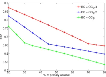
Fig. 3. Single scattering albedo at the 550 nm wavelength versus percentage of primary aerosol for 3 different core compositions with a median radius of 0.15 µm and a geometric standard deviation of 1.65.
to the same median radius of 0.045 µm and the three geo-metric standard deviation are overlaid in red blue and green. The mass extinction efficiency results from the integration of the extinction efficiency multiplied by the size distribution (and a factor ofπ r2). Figure 2 shows that the non-linearity of the extinction efficiency versus the median or effective radius mainly comes from the high fluctuations of the extinction ef-ficiency up to 2 µm.
2.2.2 Sensitivity to chemical composition
The influence of the chemical composition of the aerosol is shown in Fig. 3. The aerosol is considered to have a fixed me-dian radius of 0.15 µm, a fixed geometric standard deviation of 1.6, and a fixed total mass concentration of 10 µg m−3.
We calculated the aerosol SSA for different refractive in-dices by using the Maxwell-Garnett equation (see Sect. 2.2), considering an aerosol composed of 20 to 80% of core (pri-mary aerosol), and 80 to 20% of a shell of secondary species composed with the following mass ratio: 0.75 NH+
4, 1 H2O, 1.35 SO2−
4 , 0.9 NO
−
3 and 1 SOA to ensure the electroneutral-ity of the secondary solution.
The resulting SSA is computed for 3 different core com-positions depending of the BC/OCp ration, and for a core proportion varying from 20 to 80% of the total aerosol mass in steps of 5%. For example, an aerosol composed of 20% primary species with BC=0.25 OCp inside the core, gives
a SSA computed at 550 nm of 0.87 whereas for an aerosol composed of 80% primary species with the same OCp/BC ratio, the SSA value at the same wavelength is 0.64.
It is noteworthy that, for the same primary mass, the core composition is also very important for the computation of the SSA. For a primary mass of 50%, and for as much BC as OCp, the SSA computed reaches 0.62 whereas, with BC=1/4 OCp the SSA value is 0.77.
This is consistent with our expectations because a low SSA means that the extinction efficiency is mainly caused by ab-sorption, and the SSA has lower values when the black car-bon concentration, which is a primary and highly absorbing component, increases.
The same phenomenon is observed at the six wavelengths considered but is not shown here.
3 Methodology for the building of the look-up tables
An analytical solution was used, employing a look-up table of aerosol optical properties and a mathematical analytical function approximating the Mie computation.
In order to minimize the number of stored terms, the con-struction of the look-up tables was adjusted in two different ways described thereafter.
3.1 Description of the polynomial interpolation method
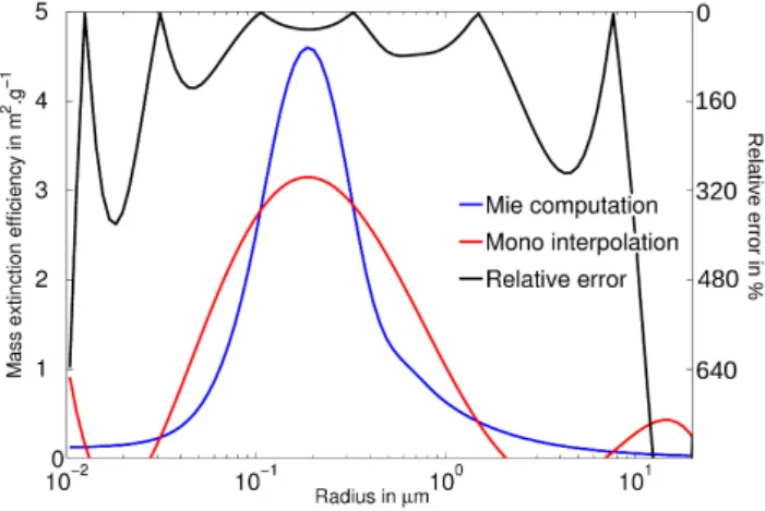
Fig. 4.Mass extinction efficiency (left) at 550 nm for given values ofσ andkr, ki as a function of the radius for the Mie computa-tion versus the mono polynomial interpolacomputa-tion and the relative error (right).
at the maximum of mass extinction efficiency. For this rea-son the interpolation of the curve was divided into two dif-ferent curves defined by the evolution from the first radius considered to radius corresponding to the maximum of the curvercut, and fromrcutto the last radius considered. Then as shown on Fig. 5, for each case considered, the two fifth de-gree polynomial coefficient and thercutwere stored. The to-tal number of stored terms was 13, which is around an eighth of the 100 stored for a discrete radius computation.
To summarize, the polynomial coefficients stored corre-sponding to the polynomialP (r)follow the equation: P (r)=
(
a10+a11r+a12r2+a13r3+a14r4+a15r5 if r < rcut a20+a21r+a22r2+a23r3+a24r4+a25r5 if r > rcut wherercutis defined as the median radius corresponding to the maximum value of the optical parameter, and the 12ai,j, withi=1,2,j=0 to 5 are stored in the look-up table. The coefficientsai,j were computed by a least square approach for the fitting of the two parts of the curve.
3.2 Range of parameters chosen
The input terms of the look-up tables are then the imaginary and real part of the complex refractive index of the aerosol, and the geometric standard deviation of the size distribu-tion. The second way to minimize the stored terms was by choosing of input terms in the look-up tables so as to obtain pseudo linearity between adjacent pairs of resulting optical properties.
Tests were performed to select a minimum amount of stored terms (not shown here), and sixki, eightkrand eight σwere chosen because of the pseudo linearity between pairs
Fig. 5.Mass extinction efficiency (left) at 550 nm for given values ofσ andkr, ki as a function of the radius for the Mie computa-tion versus the dual polynomial interpolacomputa-tion and the relative error (right).
Table 2.Input stored terms into the look-up tables for the polyno-mial interpolation.
kr ki σ λ 1.45 −0.001 1.05 217.5 nm 1.50 −0.006 1.25 345 nm 1.55 −0.008 1.45 550 nm 1.60 −0.02 1.65 925 nm 1.65 −0.1 1.85 2.285 µm 1.70 −0.4 2.05 3.19 µm
1.75 × 2.25 ×
1.80 × 2.45 ×
of terms. This selection method allowed us to interpolate be-tween the results of each optical property corresponding to the two stored values. The stored terms of the input parame-ters as well as the 6 wavelengths are reproduced in Table 2. As an example, if the value of the geometric standard devia-tion is 1.52, the corresponding aerosol optical properties are the weighted interpolations between the optical properties corresponding to the stored geometric standard deviations of 1.45 and 1.65.
3.3 Evaluation of the method in regard of direct Mie computations
In order to evaluate the dual polynomial interpolation method, a comparison between the resulting and the di-rect Mie computed aerosol optical properties was performed. This comparison was done at the 6 previously explicitedλ, for 100 considered values of median radii, and for 20 kr, 20ki and 18σ equally spaced in order not to be located at the stored values, leading to 4 320 000 comparison points for the 3 optical parameters. Because the computed parameters stands for values ofkr,ki andσ which require an interpola-tion by the module (they do not match to the stored values), this comparison allows to evaluate the module in regard of both polynomial interpolation method and choice of input stored terms.
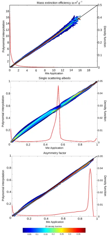
Figure 6 shows the result of the comparison for the three optical properties between the dual polynomial interpolation module and the direct Mie application. On the top (respec-tively middle and bottom) is represented the mass extinc-tion efficiency, single scattering albedo and asymmetry pa-rameter, computed by the dual polynomial interpolation as a function of the same parameter computed from the direct Mie application. Due to the very high number of scatter plots (4 320 000 for each optical parameter), the compari-son is shown as a 2-D density function computed over 100 equally splitted bins. For each bin, the 2-D density function is computed as a function of the number of sampling included in the bin. The first coloured contour (dark blue) stands for 99% of the optical parameters computed by the dual polyno-mial interpolation included within the area. The 1-D density function of the Mie computed optical parameters are repre-sented by the continuous red lines and shows to which optical parameter values do the most cases stand for. The 1-D den-sity function is computed as a function of the total number of sampling.
First, Fig. 6 shows that for the three optical parame-ter computations, the dual polynomial inparame-terpolation method manages to reproduce the values computed by the direct Mie application. Indeed, almost all of the parameters computed by the module follow the linear curvex=y represented by a continuous black line. The correlation coefficients value standing for the three optical parameters are respectively 0.9992, 0.9946 and 0.9994. The most large differences stand for extreme cases with very low median radius or very high geometric standard deviation. As an example, the highest values of mass extinction efficiencies which can reach more than 15 g m−2stand for very unusual combinations of param-eters such as a geometric standard deviation below 1.4, a real part of the refractive index of 1.80. These extreme cases all occur on the first wavelength. We can also notice that for the single scattering albedo, the highest dispersion stand for very low values, meaning that the extinction is mainly ab-sorbing. Moreover, the most computed cases, represented by the continuous red line, occur where the density function is
the highest, and at this points there is a good linearity be-tween the two methods.
4 Validation during the EUCAARI campaign
For the validation of the module, a full set of measured data for the inputs and of the outputs was required. Concerning inputs, a description of the aerosol size distribution giving the median radius and the geometric standard deviation for each mode, associated with the aerosol chemistry giving the aerosol composition was needed. Concerning outputs, the measurements of the aerosol optical properties was also nec-essary.
During the EUCAARI field experiment, a complete set of instruments were available at the Cabauw tower. Between 15 and 29 May 2008, all the selected instruments requested to test this module were operational.
4.1 Description of observations
4.1.1 Period and instruments
The data were processed to give one average value over 30 min for each parameter during the 15 days.
– The aerosol size distribution was deduced after merg-ing the size spectral observations from a SMPS (model TSI 3034) and an APS (model TSI 3321): the SMPS measures the aerosol size distribution between 10 and 500 nm, and the APS between 500 nm and 20 µm. All the measurements were made in dry conditions (RH<50%).
Then, a lognormal fit that best approached the observed distribution was found. At each time step, a least square approach gave the median radius, the geomet-ric standard deviation and the mass concentration for each aerosol mode observed by both instruments. To link the number of aerosol directly measured to the mass of aerosol, the assumption of spherical particles with a density of 2.5 g cm−3was done.
– The chemical composition of the aerosol was deduced from the observations of an aerosol mass spectrome-ter (AMS, cTOF type) and a multi angle absorption photometer (MAAP model 5012). The AMS gave us the mass concentration of particulate organic matter (POM), NO−
3, NH
+
4, SO2
−
4 at each time step and the black carbon (BC) concentration was deduced form the MAAP measurements. The water concentration was de-duced from the thermodynamical equilibrium EQSAM (Metzger et al., 2002) on dry conditions.
– The scattering coefficient at 550 nm was measured by a nephelometer (model TSI 3563). A truncation cor-rection is performed on the nephelometer data accord-ing to Mallet et al. (2009). The absorption coefficient
was measured by the MAAP at 670 nm and deduced at 550 nm by using the absorption Angstr¨om coefficient measured with an aethalometer. All these measure-ments were also made in dry conditions.
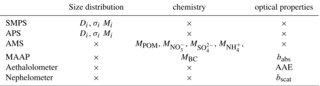
A summary of the instruments and the associated aerosol properties is presented in Table 3.
4.1.2 Methodology and assumptions
Figure 7 shows as a diagram the methodology used for the validation of the radiative module. Some assumptions were made from the observations. The choice was to split the POM between primary organic carbon and secondary organic carbon with a 60–40% distribution according to Dentener et al. (2006). A second assumption was to split the aerosol compounds equally between modes. The SMPS+APS observations are fitted to describe the aerosol mass size distribution along three lognormal modes: Mi,σi,ri withi for the mode index. This fit is performed according to two assumptions allowing to compute the mass concentration from the observed number concentration: the aerosol is supposed to be spherical and has a constant density ρ. From this fit is also deduced the total aerosol mass concentrationMsd and the aerosol mass concentration integrated from 0.01 to 0.5 µm (Msd,500). The particle organic matter, ammonium, nitrate, sulfate, and black carbon mass concentration are deduced from the AMS+MAAP observations (respectively MPOM, MNH4, MSO4, MNO3,
MBC). It was noticed that the AMS had a cut-off diameter of 500 nm. The total aerosol mass concentration for aerosols with a diameter inferior to 500 nm and as observed by the AMS+MAAP is also computed (Mch,500). Then, for each of the three considered mode, the mass concentration of each aerosol compounds is computed and weighted by the total mass concentration observed by the SMPS+APS (MPOM,i, MNH4,i,MSO4,i,MNO3,i,MBC,i). The inputs for the radiative
module are then for each mode: MPOM,i, MNH4,i, MSO4,i,
MNO3,i, MBC,i, ri, σi. The outputs are then for each of
Fig. 7.Diagram representation of the methodology used for the validation.ρis the density considered for the aerosol particle.iis the index of the aerosol lognormal mode. Mi is the aerosol mass concentration value for thei-th mode obtained from the lognormal fit adjusted on the SMPS+APS size distribution observations.Msdis the total mass concentration deduced from the fit of the SMPS+APS size distribution observations. Msd,500is the mass concentration calculated from the fit of the SMPS+APS size distribution observations integrated up to 500 nm.MPOM,MNH4,MSO4,MNO3, is the particle organic matter, ammonium, sulfate, nitrate mass concentration respectively measured by the AMS.MBCis the black carbon mass concentration deduced from the MAAP.Mch,500is the mass concentration deduced from the AMS+MAAP observations up to 500 nm. babs,obs,670is the absorption coefficient measured by the MAAP at the wavelength of 670 nm. AAEabs,obsis the absorption Angstr¨om coefficient measured by the aethalometer. MEE is th Mass extinction efficiency.
Table 3.Summary of aerosol measurements on Cabauw tower during the EUCAARI campaign.
Size distribution chemistry optical properties
SMPS Di,σiMi × ×
APS Di,σiMi × ×
AMS × MPOM,MNO−
3,MSO2
−
4 ,
MNH+
4,
×
MAAP × MBC babs
Aethalolometer × × AAE
Nephelometer × × bscat
4.1.3 First results from instruments
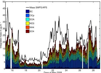
The 15-day period of the study showed different aerosol con-centration level due to different regimes. As presented in Fig. 8, the aerosol composition gives us several items of in-formation: from 15 to 17 May, the aerosol shows a continen-tal composition; from 17 to 21 May, the low level of aerosols is characteristic of a scavenging period with a clean air mass and fresh aerosols; from 21 to 29 May, the aerosol comes again from a continental air flux and the secondary fraction of the aerosol, in particular the inorganic species, also grows in proportion. The total measured mass concentration is also represented in Fig. 8 as a black line. Also one can note that the ratio of primary aerosol to secondary aerosol remains quite stable during the fourteen days of measurements.
Figure 9 shows the evolution of the aerosol size distribu-tion during the fourteen days of measurement. This figure is
the result of the fit applied to the SMPS+APS data and used as inputs in the module.
The Fig. 9 shows the evolution of all the size distribution parameters versus time. The maximum of mass also evolves consequently as already shown in Fig. 8. Finally, the combi-nation of data measuring size description and chemical com-position gives a good representation of the period.
16 18 20 22 24 26 28 0
5 10 15 20 25 30 35 40 45 50
Days of May 2008
Integrated mass in
µ
g.m
−3
Mass SMPS/APS
BC
OCp
SOA
NO3
NH4
SO4
Fig. 8. Evolution of aerosol chemical composition from AMS+MAAP and mass integrated from the SMPS and APS in µg m−3during the fourteen days of measurement.
4.2 Comparison of computed optical properties and observations
Figure 10 shows the single scattering albedo at 550 nm as cal-culated form the nephelometer and the MAAP measurements (continuous red line) and computed by the module (dashed blue line).
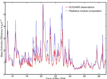
Figure 11 shows the mass extinction efficiency at 550 nm as calculated from observations (continuous red line) and computed by the module (dashed blue line). There were no instruments able to measure the asymmetry parameter during the EUCAARI campaign. Therefore, there is no comparison possible with the computed values.
First, the main trend shows that both mass extinction effi-ciency and single scattering albedo are correctly reproduced by the module during the 15 days. The correlation coefficient for the 15-day period and for the mass extinction efficiency is 0.94, and 0.89 for the single scattering albedo and the as-sociated biases are 0.32 and 0.0025, respectively.
Concerning the single scattering albedo, the module mainly manages to reproduce the highest as the lowest val-ues observed, even with high temporal variability. Single scattering albedo values observed and modelled in dry condi-tions fluctuate around 0.8 (with a mean value of 0.815 for the modelled values and 0.818 for the observed values during the period studied). However, some isolated measurements show low values of single scattering albedo below 0.7. Al-though such very low values could be unusual, recent studies (Marley et al., 2009; Gomes et al., 2008; Babu et al., 2002; Singh et al., 2005; Ganguly et al., 2006) show single scat-tering albedo observations showing chronic very low values below 0.6 indicating an higher concentration of absorbing aerosols. In addition, it has to be noted that the SSA ob-served and modelled are both under dry conditions, leading to lower SSA values compared to wet conditions.
Fig. 9. Evolution of aerosol size distribution fits obtained from SMPS+APS during the fourteen days of measurement.
16 18 20 22 24 26 28
0.5 0.6 0.7 0.8 0.9 1
Days of May 2008
Single Scattering Albedo
Nephelometer+MAAP observations Radiative module computation
Fig. 10. Evolution of the dry single scattering albedo at 550 nm measured at Cabauw during EUCAARI by the nephelometer and the MAAP, and computed by the module.
Concerning the mass extinction efficiency comparison, again there is a good agreement between the observations and the computations. However, it is noticeable that from 20 to 24 May, the computations overestimate the mass extinction efficiency by 10 to 80%. To understand why there is a less good correlation especially between 20 and 24 May, Fig. 12 shows the evolution of the difference between the observed and computed mass extinction efficiency (in red) during the 15-day period, and the evolution of the relative error on the integrated mass up to 500 nm observed by the SMPS+APS
Msd,500and by the AMS+MAAPMch,500.
16 18 20 22 24 26 28 0
1 2 3 4 5 6
Days of May 2008
Mass Extinction Efficiency in g.m
−2
EUCAARI observations Radiative module computation
Fig. 11.Evolution of the dry mass extinction efficiency in g m−2at 550 nm measured at Cabauw during EUCAARI and computed by the module.
Fig. 12. Relative error between the mass concentration measured by the AMS+MAAP and that deduced from the SMPS+APS for particles up to 500 nm (blue line) and difference between mass ex-tinction efficiency observed and computed (red line).
chemical composition. Between 20 and 24 May, the relative error between both systems on the aerosol integrated mass up to 500 nm can reach more than 100% and the major differ-ences between the observed and computed mass extinction efficiency occur at these same maxima. Thus, the main dif-ferences observed may probably come from a discrepancy in the instruments in term of mass measurement, leading to an inconsistency between the inputs and outputs of the module. Moreover, the constant density used for the computations of the module’s inputs certainly leads to the main limitation of this evaluation.
5 Conclusions
In order to quantify the direct and semi-direct effect of aerosols, it is necessary to compute the aerosol optical pro-perties in atmospheric models depending on an evolving and complex aerosol particle. To study the aerosol particles inter-action with radiation in highly temporal and spatial variable locations, such as urban areas, it is necessary to consider a large number of chemical species.
Nevertheless, the high computing cost of the classi-cally applied Mie theory generally leads to a climatologi-cal parametrization of aerosol opticlimatologi-cal properties in regional-climate models.
The numerical computation was performed for six wave-lengths using a vectorial computer (NEC SX8 type), in order to compare the time cost of this module with the other atmo-spheric processes (turbulence, advection, chemistry, aerosol solver, etc.).
The comparison was made between two standard simu-lations, with and without computation of the aerosol opti-cal properties. The standard simulation required a cpu time per point per time-step of 98.0 µs versus the standard simula-tion with the aerosol optical properties computasimula-tion has a cpu time per point per time-step of 99.7 µs. These results show that the numerical cost of the module was no more than 1.7% of the standard simulation total cost. As an example, the chemistry solving cost of these same simulations is 35.6%.
We can then consider that the previously described module is numerically very cheap relative to other processes and is consequently affordable for most atmospheric modelling.
This work presents a new, computationally cheap module dedicated to the online computation of optical properties ac-cording to the particle chemical composition and size distri-bution.
To minimize the computing cost, the module is founded on look-up tables built by a dual fifth degree polynomial inter-polation of the parameters depending on the median radius of the aerosol size distribution. The parameters are the geo-metric standard deviation of the lognormal size distribution of the aerosol mode considered, and the imaginary and real part of the complex aerosol refractive index corresponding to a chemical composition deduced from the Maxwell-Garnett equation.
The module was then evaluated by using observations ac-quired during the EUCAARI campaign (May 2008). The nu-merical cost was also tested.
1998). This development will be used in future works to investigate feedbacks of polluted aerosols on radiation and urban climate (especially impacts on radiative heating, de-velopment of the urban boundary layer and the urban breeze). Such a model could also be used for studying the effect of ur-ban aerosols on UV radiation and the possible feedbacks on atmospheric photochemistry (such as the ozone production) in urban zones.
Supplement related to this article is available online at: http://www.geosci-model-dev.net/3/553/2010/
gmd-3-553-2010-supplement.zip.
Acknowledgements. This work has been partially funded by
Eu-ropean Commission 6th Framework program project EUCAARI, contract no. 036833-2 (EUCAARI), and by the French National Research Agency (ANR) under the AEROCLOUD program, con-tract no. 06-BLAN-0209. Astrid Kiendler-Scharr from Research Center Juelich, Germany, is acknowledged for providing AMS data. The Meso-NH team is also acknowledged for its support. The topical editor O. Boucher is also acknowledged for his constructive remarks improving this manuscript.
O. Boucher
The publication of this article is financed by CNRS-INSU.
References
Babu, SS., Satheesh, S.K., and Moorthy, K.K.: Aerosol radiative forcing due to enhanced black carbon at an urban site in India, J. Geophys. Res., 29, 1880, doi:10.1029/2002GL015826, 2006. Chylek, P., Videen, G., Geldart, W., Dobbie, S., and Tso, W.:
Ef-fective medium approximation for heterogeneous particles, in: Light Scattering by Nonspherical Particles: Theory, Meas. Geo-phys. Appl., 273–308, 2000.
Costabile, F., Birmili, W., Klose, S., Tuch, T., Wehner, B., Wieden-sohler, A., Franck, U., K¨onig, K., and Sonntag, A.: Spatio-temporal variability and principal components of the particle number size distribution in an urban atmosphere, Atmos. Chem. Phys., 9, 3163–3195, doi:10.5194/acp-9-3163-2009, 2009. Dentener, F., Kinne, S., Bond, T., Boucher, O., Cofala, J.,
Gen-eroso, S., Ginoux, P., Gong, S., Hoelzemann, J.J., Ito, A., Marelli, L., Penner, J.E., Putaud, J.P., Textor, C., Schulz, M., van der Werf, G.R., and Wilson, J.: Emissions of primary aerosol and precursor gases in the years 2000 and 1750 prescribed data-sets for AeroCom, Atmos. Chem. Phys., 6, 4321–4344, doi:10.5194/acp-6-4321-2006, 2006.
Forster, P., Ramaswamy, V., Artaxo, P., Berntsen, T., Betts, R., Fa-hey, D., Haywood, J., Lean, J., Lowe, D., Myrhe, G., Nganga, J., Prinn, R., Raga, G., Schulz, M., and van Dorland, R.: Changes
in atmospheric constituents and in radiative forcing, in: Climate Change 2007: The Physical Science Basis, Contribution of work-ing group I to the fourth assessment report of the intergovern-mental panel on climate change, edited by: Solomon, S., Qin, D., Manning, M., Chen, Z., Marquis, M., Averyt, K. B., Tignor, M., and Miller, H. L., Cambridge University Press, 2007.
Ganguly, D., Jayaraman, A., Rajesh, T.A., and Gadhavi, H.: DWintertime aerosol properties during foggy and nonfoggy days over urban center Delhi and their implications for short-wave radiative forcing, J. Geophys. Res., 111, D15217, doi:10.1029/2005JD007029, 2006.
Gomes, L., Mallet, M., Roger, J.C., and Dubuisson, P.: Effects of the physical and optical properties of urban aerosols measured during the CAPITOUL summer campaign on the local direct ra-diative forcing, Meteorol. Atmos. Phys., 108, 289–306, 2008. Grini, A., Tulet, P., and Gomes, L.: Dusty weather forecast using the
MesoNH atmospheric model., J. Geophys. Res., 111, D19205, doi:10.1029/2005JD007007, 2006.
IPCC (Ed.): Climate change 2007: The scientific basis. Contribu-tion of working group I to the Fourth Assessment Report of the Intergovernmental Panel on Climate Change, http://www.ipcc. ch/, last access: 27 May 2010, 2007.
Jacobson, M.: A physically-based treatment of elemental carbon optics: Implications for global direct forcing of aerosols, Geo-phys. Res. Lett., 27, 217–220, 2000.
Kinne, S., Schulz, M., Textor, C., Guibert, S., Balkanski, Y., Bauer, S. E., Berntsen, T., Berglen, T. F., Boucher, O., Chin, M., Collins, W., Dentener, F., Diehl, T., Easter, R., Feichter, J., Fillmore, D., Ghan, S., Ginoux, P., Gong, S., Grini, A., Hen-dricks, J., Herzog, M., Horowitz, L., Isaksen, I., Iversen, T., Kirkev˚ag, A., Kloster, S., Koch, D., Kristjansson, J. E., Krol, M., Lauer, A., Lamarque, J. F., Lesins, G., Liu, X., Lohmann, U., Montanaro, V., Myhre, G., Penner, J., Pitari, G., Reddy, S., Se-land, O., Stier, P., Takemura, T., and Tie, X.: An AeroCom ini-tial assessment – optical properties in aerosol component mod-ules of global models, Atmos. Chem. Phys., 6, 1815–1834, doi:10.5194/acp-6-1815-2006, 2006.
Krekov, M.: Aerosols Effects on Climate, Univerity of Arizona Press, USA, 9–72, 1993.
Kulmala, M., Asmi, A., Lappalainen, H. K., Carslaw, K. S., P¨oschl, U., Baltensperger, U., Hov, Ø., Brenquier, J.-L., Pan-dis, S. N., Facchini, M. C., Hansson, H.-C., Wiedensohler, A., and O’Dowd, C. D.: Introduction: European Integrated Project on Aerosol Cloud Climate and Air Quality interactions (EU-CAARI) – integrating aerosol research from nano to global scales, Atmos. Chem. Phys., 9, 2825–2841, doi:10.5194/acp-9-2825-2009, 2009.
Lafore, J. P., Stein, J., Asencio, N., Bougeault, P., Ducrocq, V., Duron, J., Fischer, C., H´ereil, P., Mascart, P., Masson, V., Pinty, J. P., Redelsperger, J. L., Richard, E., and Vil`a-Guerau de Arel-lano, J.: The Meso-NH Atmospheric Simulation System. Part I: adiabatic formulation and control simulations, Ann. Geophys., 16, 90–109, doi:10.1007/s00585-997-0090-6, 1998.
Lesins, G., Chylek, P., and Lohmann, U.: A study of internal and external mixing scenarios and its effect on aerosol optical pro-perties and direct radiative forcing, J. Geophys. Res., 107(D10), 4094, doi:10.1029/2001JD000973, 2002.
properties during photochemical pollution events, J. Geophys. Res., 110, D03205, doi:10.1029/2004JD005139, 2005.
Marley, N.A., Gaffney, J.S., Castro, T., Salcido, A., and Freder-ick, J.:Measurements of aerosol absorption and scattering in the Mexico City Metropolitan Area during the MILAGRO field cam-paign: a comparison of results from the T0 and T1 sites, Atmos. Chem. Phys., 9, 186–206, doi:10.5194/acp-9-186-2009, 2009. Maxwell-Garnett, J.: Colours in metal glasses and in metallic films,
Philos. T. Roy. Soc. A, 203, 385–420, 1904.
Metzger, S., Dentener, F., Pandis, S., and Lelieveld, J.: Gas/aerosol partitioning: 1. A computationally efficient model, J. Geophys. Res., 107(D16), 4312, doi:10.1029/2002GL014769, 2002. Mie, G.: Beitr¨age zur Optik tr¨uber Medien, speziell kolloidaler
Metall¨osungen, Ann. Phys.-Leipzig, 330, 377–445, 1908. Mikhailov, E. F., Vlasenko, S. S., Podgorny, I. A., Ramanathan, V.,
and Corrigan, C. E.: Optical properties of soot water drop agglomerates: An experimental study, J. Geophys. Res., 111, 1815–1834, doi:10.1029/2005JD006389, 2006.
Raut, J.-C. and Chazette, P.: Vertical profiles of urban aerosol com-plex refractive index in the frame of ESQUIF airborne mea-surements, Atmos. Chem. Phys., 8, 901–919, doi:10.5194/acp-8-901-2008, 2008.
Russell, P. B., Bergstrom, R. W., Shinozuka, Y., Clarke, A. D., DeCarlo, P. F., Jimenez, J. L., Livingston, J.M., Redemann, J., Dubovik, O., and Strawa, A.: Absorption Angstrom Exponent in AERONET and related data as an indicator of aerosol composi-tion, Atmos. Chem. Phys., 10, 1155–1169, 2010,
http://www.atmos-chem-phys.net/10/1155/2010/.
Seinfeld, J. and Pandis, S.: Atmospheric Chemistry and Physics, Wiley Interscience Pub., New York, USA, 691–711, 1997.
Singh, S., Nath, S., Kohli, R., and Singh, R.: Aerosols over Delhi during pre-monsoon months: Characteristics and effects on surface radiation forcing, Geophys. Res. Lett., 32, L13808, doi:10.1029/2005GL023062, 2005
Solmon, F., Chuang, P., Meskhidze, N., and Chen, Y.: Acidic processing of mineral dust iron by anthropogenic compounds over the North Pacific Ocean, J. Geophys. Res., 114, D02305, doi:10.1029/2008JD010417, 2008.
Tombette, M., Chazette, P., Sportisse, B., and Roustan, Y.: Simu-lation of aerosol optical properties over Europe with a 3-D size-resolved aerosol model: comparisons with AERONET data, At-mos. Chem. Phys., 8, 7115–7132, doi:10.5194/acp-8-7115-2008, 2008.
Tulet, P., Crassier, V., Cousin, F., Shure, K., and Rosset, R.: ORILAM, a three moment lognormal aerosol scheme for mesoscale atmospheric model. On-line coupling into the MesoNH-C model and validation on the ESCOMPTE campaign, J. Geophys. Res., 110, D18201, doi:10.1029/2004JD005716, 2005.
Tulet, P., Grini, A., Griffin, R., and Petitcol, S.: ORILAM-SOA: a computationally efficient model for predicting secondary or-ganic aerosols in 3D atmospheric models., J. Geophys. Res., 111, D23208, doi:10.1029/2006JD007152, 2006.