Particle size distributions by laser diffraction: sensitivity of granular matter strength to analytical operating procedures

(1)

www.solid-earth.net/1/25/2010/

Solid Earth

Particle size distributions by laser diffraction: sensitivity of

granular matter strength to analytical operating procedures

F. Storti and F. Balsamo

Dipartimento di Scienze Geologiche, Universit`a “Roma Tre”, Largo S. L. Murialdo 1, 00146 Roma, Italy Received: 6 November 2009 – Published in Solid Earth Discuss.: 21 December 2009

Revised: 24 March 2010 – Accepted: 2 April 2010 – Published: 19 April 2010

Abstract. We tested laser diffraction particle size analy-sis in poorly coherent carbonate platform cataclastic brec-cias and unfaulted quartz-rich eolian sands, representing low-and high-strength granular materials, respectively. We used two different instruments with different sample dispersion and pumping systems and several wet analytical procedures that included different pump speeds, measurement precision tests with and without sample ultrasonication, and different dispersant liquids. Results of our work indicate that high strength material is not strongly affected by analytical op-erating procedures, whereas low strength materials are very sensitive to the pump speed, ultrasonication intensity, and measurement run time. To reduce such a data variability, we propose a workflow of analytical tests preliminary to the set up of the most appropriate SOP.

1 Introduction

Particle size distributions provide fundamental information for rock characterization and geological process descrip-tion in earth sciences, including sedimentology, stratigraphy, structural geology, pedology, and volcanology (e.g. Krum-bein, 1941; Irani and Callis, 1963; Engelder, 1974; Fried-man, 1979; Sheridan et al., 1987; Rieu and Sposito, 1991). In the last three decades, laser diffraction particle size analy-sers have proved to be an effective tool for providing particle size distributions of poorly coherent rocks and soils (Weiss and Frock, 1976; McCave et al., 1986; de Boer et al., 1987; Wanogho et al., 1987; Agrawal et al., 1991; Loizeau et al., 1994; Pye and Blott, 2004; Blott and Pye, 2006). This is be-cause they require little time for analysis, cover a wide size range, and require small size samples (e.g. Beuselinck et al.,

Correspondence to:F. Storti (storti@uniroma3.it)

1998), thus facilitating very detailed studies of particle size distributions in geological structures.

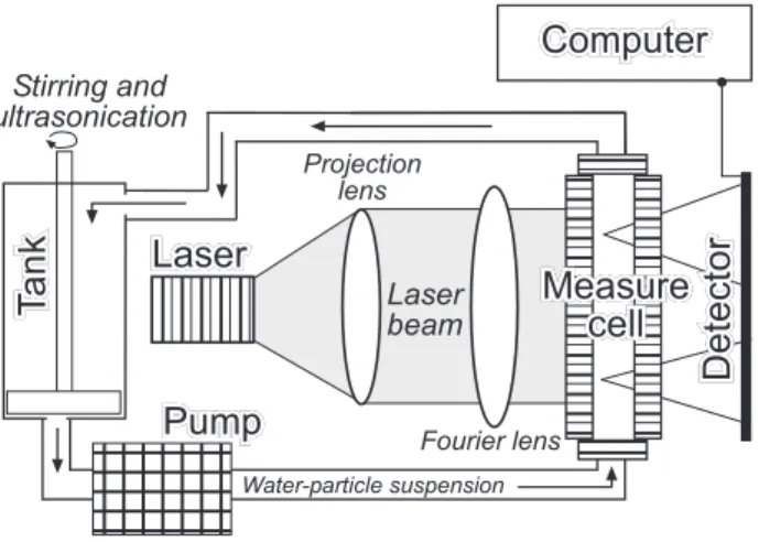
Laser diffraction particle size analysers provide indirect size measurements of spherically equivalent particles, based on the principle that particles of a given size diffract light through a given angle that increases logarithmically with de-creasing size (e.g. Beuselinck et al., 1998). In “wet proce-dures”, a few grams of material are dispersed into a liquid that circulates across a quartz measurement cell illuminated by a laser beam (Fig. 1). Different instruments have dif-ferently designed systems for stirring the dispersant liquid into the tank and ensuring its circulation through the mea-surement cell by mechanical pumping. A wide variety of standard operating procedures (SOP) can be set up in laser diffraction particle size analysers. They include the pump speed, the number of measurement runs, the length of the measurement time, and the use of dispersing agents and/or ultrasonication to aid sample disaggregation and dispersion (e.g. Blott et al., 2004; Sperazza et al., 2004). It follows that measurement results, particularly when dealing with datasets produced by different operators and/or different instruments, can be influenced by the adopted SOP. Sample ultrasonica-tion, for example, can aid particle disaggregation by collision or, in some cases, particle agglomeration (e.g. Mason et al., 2003; Blott et al., 2004).

(2)

Laser

Laser beam Projection

lens

Fourier lens

Water-particle suspension Stirring and

ultrasonication

T

ank

Measure

cell

Pump

Detector

Computer

Fig. 1.Schematic cartoon showing the main components of a laser diffraction particle size analyser. See text for details.

in granular rocks. The proposed testing procedure can result appropriate for a wide variety of rock types, including cata-clastic rocks in fault zones and cata-clastic sediments that under-went burial-related grain microfracturing.

2 Instruments overview

Most granulometric analyses were performed with a Mas-tersizer 2000 laser diffraction granulometer and associated dispersion units manufactured by Malvern Instruments Ltd. This laser diffraction particle size analyser is designed for measuring particle sizes in the 0.02 to 2000 µm range by us-ing a blue (488.0 µm wavelength LED) and red (633.8 µm wavelength He-Ne laser) light dual-wavelength, single-lens detection system. The light energy diffracted by the di-lute suspension circulating through the cell is measured by 52 sensors. The light intensity adsorbed by the material is measured asobscurationand indicates the amount of sam-ple added to the dispersant liquid. Light scattering data are accumulated in 100 size fractions bins, which are analysed at 1000 readings per second, and compiled with Malvern’s Mastersizer 2000 software by using either full Mie or Fraun-hofer diffraction theories (de Boer et al., 1987). Light scatter-ing data acquired by the Mastersizer 2000 granulometer were all mathematically inverted using the Mie theory, which uti-lizes the refractive index (RI) and absorption (ABS) of the dispersed granular material, and RI of the dispersant liquid. This theory is based on the assumption that: (1) particles are mineralogically homogeneous; (2) particles are spherical; (3) the optical properties of particle and dispersion medium are known; (4) suspension dilution guarantees that light scat-tered by one particles is measured before being-re-scatscat-tered by other particles.

Particle size distributions were measured from wet disper-sions using both small (Malvern Hydro 2000 S) and large (Malvern Hydro 2000 MU) volume sample dispersion units available for the Mastersizer 2000 granulometer. The Hy-dro 2000 S unit has a capacity of 50 to 120 ml and is equipped with a continuously variable single shaft centrifugal pump and stirrer (up to 3500 revolutions per minute; in the follow-ing rpm), and by a continuously variable ultrasonic probe. The Hydro 2000 MU unit has a dispersion mechanism con-sisting of a sample recirculation head immerged into a stan-dard laboratory beaker (capacity of 600 to 1000 ml), which contains a built-in stirrer and sample recirculation centrifu-gal pump (from 600 to 4000 rpm), and a continuously vari-able ultrasonic probe (maximum power is 20 µm of tip dis-placement). A comparative wet analysis was performed by a Cilas 930 laser diffraction granulometer manufactured by Cilas, which measures particle size distributions in the 0.2 to 500 µm size range of wet dispersions by diffraction of a laser light of 830 nm wavelength, based either on the Fraunhofer or Mie diffraction theories. Sample recirculation is achieved by two peristaltic pumps.

The analysed carbonate fault breccia sample, named CABRE3, was collected in the same site of sample CABRE1 described in Storti and Balsamo (2010), and was sieved at 500 µm to account for the analytical size range of the Cilas 930 laser diffraction particle size analyser. Repro-ducible sub-sampling up to about 20 g weight of the total sample amount was achieved by using a Quantachrome Siev-ing Riffler-Rotary Sample Splitter. Sub-sample aliquots nec-essary to produce laser obscuration values between 10% and 15% were randomly selected from sub-samples (from 0.5 g to few grams) and added into the liquid-filled beaker for anal-ysis.

3 Factors influencing data acquisition and processing from dilute suspensions: testing strategy

(3)

(sub-sample aliquots CABRE3x): pump speed test, measure-ment precision test (instrumeasure-ment precision test of Blott et al., 2004), ultrasonication test, chemical test, and reprocessing test.

The pump speed test is labelled Pt-test, wheretis the

mea-surement run time (i.e. the number of readings that are aver-aged in a single measurement), and consists of measurement runs performed on a given sub-sample aliquot, at different stirrer and pump speed (in the following simply referred to as pump speed) for a givent. The test starts with the set up of laser obscuration values between 10% and 15% at half of the maximum pump speed. The pump speed is then lowered to the minimum value and few (typically 10) measurement runs are performed before increasing the pump speed (typically by 100 rpm). Progressive measurement steps are carried out up to the maximum pump speed. Results are plotted in a mean diameter versus pump speed graph to select the most appropriate rpm value for further analyses. The measurement precision test is labelled MPtS, whereSis the pump speed,

and consists of measurement runs acquired at given pump speed and measurement run time during sub-sample recir-culation through the measurement cell. Our MPtS analyses

typically consisted of 100 measurement runs, which means some hundred thousands of instrument readings. Analysis of data trends is included in the measurement precision test to help selecting the most appropriate number of measurement runs and to prevent significant mechanical bias. Addition of sub-sample ultrasonication to the measurement precision test produces the ultrasonication test US, which is labelled as USdS, whered is the probe tip displacement in the

Hy-dro 2000 MU dispersion unit. Chemical effects were inves-tigated by repeating the above mentioned sample tests using different dispersion liquids. The suffixlis added to the ap-propriate test labelling in order to indicate the dispersion liq-uid used, which can be a solution with a dispersing agent. We did not use specific labelling for decalcified tap water by cou-pled magnetic and chemical commercial devices, which was used in most of our analyses. The reprocessing test consists of changing the optical properties of both granular material and dispersant liquid during light scattering data processing of a given analysis by the Mie theory through the Master-sizer 2000 software.

Our preferred workflow (Fig. 2) starts with a pump speed test to provide indications on the pump speed range for fur-ther testing. Short measurement run times (typically 5 s as a starting value) are used in pump speed analyses, in order to minimise sub-sample mechanical alteration without com-promising the statistical robustness of the data. Results from the P-test provide constraints for MP and US test pairs per-formed at the same pump speed values. More than one test pair can be performed to investigate uncertainties associated with the pump test. Cross checking of results from the MP and US tests is commonly achieved by comparing the be-haviour of mean diameters, of the corresponding laser ob-scuration values, and of other statistical parameters including

pump speed range

1 n

MPt_S1

+

USd_S1

P testt

MPt_Sn

+

USd_Sn

best sample recirculation and measure run time parameters

Chemical test

best dispersant liquid

SP test

Final

SOP

P = pump speed test

MP = measurement precision test US = Ultrasonication test

t = measurement run time s = pump speed d = probe tip displacement

Reprocessing test

Fig. 2.Flow chart illustrating the main steps that constitute the pro-posed workflow to select the most appropriate operating procedure for analyzing granular materials. See text for details.

the mode and percentiles, among whichD10,D50, andD90

are the most common ones. Once the most appropriate pa-rameters in terms of best sample recirculation, measurement run time, and measurement run number are selected, all in-formation for defining the most appropriate SOP is available for a given dispersion liquid. The next step is to check the effectiveness of the selected dispersion medium by running the same test with different dispersion liquids. Comparison of all results leads to the selection of the final SOP, which can be repeated for several sub-samples to perform a sam-pling precision test (Blott et al., 2004) that allows evaluating measurement reproducibility (Fig. 2).

(4)

a

b

c

0 1000 2000 3000 4000

0 100 200 300 400 500

Pump speed (revolutions per minute)

Mean diameter (

m

m)

0 1000 2000 3000 4000

0 2 6 8 10 12 14 16 18

Obscuration (%)

0 1000 2000 3000 4000

0 200 400 600 800

Diameter (

m

m)

Pump speed (revolutions per minute) D50

D10 D90

d

Log Particle Size (mm)

V

olume percent

age

0.01 0.1 1 10 100 1000

6 9 12 18

3

0

900 rpm

1400 rpm 1500 rpm 1000 rpm 1100 rpm 1200 rpm 1300 rpm

2500 rpm 3000 rpm 3500 rpm 4000 rpm 2000 rpm

15 clay size

silt size sand size

V

olume percent

age

Pump speed (rpm)

0 1000 2000 3000 4000

0 20 40 60 80 100

e

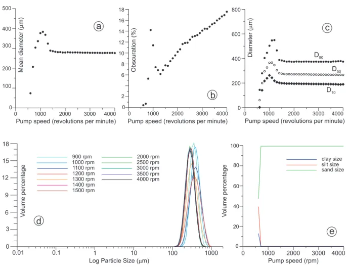
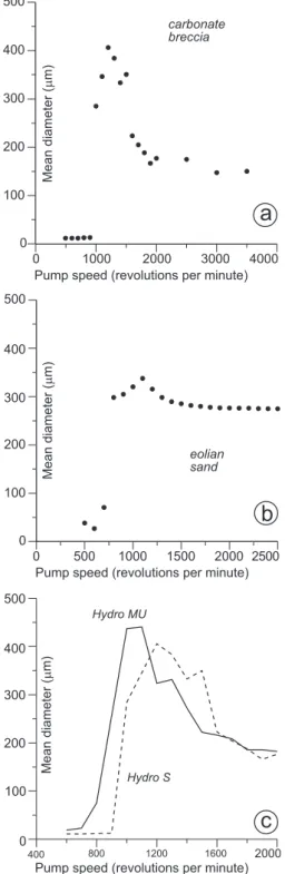
Fig. 3. Results of the pump speed test P5performed on sub-sample aliquot SAND1a by the Hydro 2000 MU dispersion unit. (a)Mean

diameter value evolution with increasing the pump speed from 600 up to 4000 rpm.(b)Laser obscuration value progression during the same test.(c)Progression ofD₁₀,D₅₀, andD₉₀during the same test.(d)Granulometric curves obtained by averaging data from the corresponding 10 measurement runs during representative pump speed steps.(e)Distribution of clay, silt, and sand size fractions during the test. Note that the sand fraction quickly reaches 100% of the sample material. See text for details.

measurement runs regardless of indications from previous tests. This because of the short time required by laser diffrac-tion particle size analysers to acquire light scattering data, thus encouraging the collection of large datasets from which sub-sets can then be easily extracted.

4 Pump speed test

Results of the P5-test of sub-sample aliquot SAND1a

(i.e. 5000 readings of the scattered light energy distribution for each measurement run) are illustrated in Fig. 3. Mean diameters show an asymmetric bell-shaped trend character-ized by very low values at 600 and 700 rpm, a maximum at 1000 to 1200 rpm, and an almost flat envelope of mean di-ameter values at pump speed higher than 1800 rpm (Fig. 3a). The corresponding laser obscuration values show a much higher variability, with a peak at 900 rpm and a minimum at 1300 rpm, followed by a near constant increase at higher

pump speed values (Fig. 3b). The trend ofD10,D50, andD90

percentile data points strongly resembles the distribution of the mean diameters (Fig. 3c). Granulometric curves averaged over 10 measurement runs indicate a strongly unimodal par-ticle size distribution with some variability of both volume percentage and modal peak size between 900 and 1500 rpm. Conversely, almost overlapping curves support strongly con-sistent results at pump speed values greater than 2000 rpm (Fig. 3d). The well sorted particle size distribution of the sample is illustrated by the pattern of clay, silt, and sand size fractions: starting from 700 rpm, the latter includes 100% of the analysed material (Fig. 3e).

The P5-test of sub-sample aliquot CABRE3a shows an

(5)

c

Diameter (

m

m)

a

0 100 200 300 400 500

0 1000 2000 3000 4000

Mean diameter (

m

m)

b

0 1000 2000 3000 4000

Obscuration (%)

0 2 4 6 8 10 12 14 16 18

0 200 400 600 800

Pump speed (revolutions per minute) D50 D10

D90

0 1000 2000 3000 4000

clay size silt size sand size

V

olume percent

age

Pump speed (rpm)

d

V

olume percent

age

0.01 0.1 1 10 100 1000

8 12 16

4

0

900 rpm

0 1000 2000 3000 4000

0 20 40 60 80

100

_e

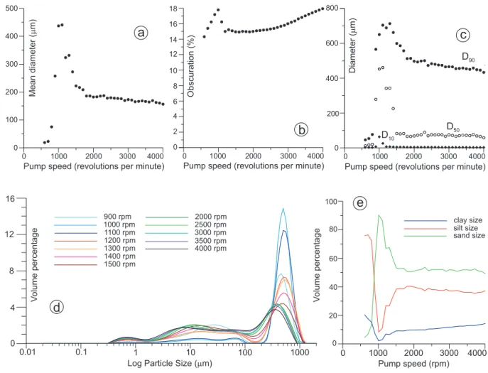
Fig. 4. Results of the pump speed test P5performed on sub-sample aliquot CABRE3a by the Hydro 2000 MU dispersion unit. (a)Mean

diameter value evolution with increasing the pump speed from 600 up to 4000 rpm.(b)Laser obscuration value progression during the same test.(c)Progression ofD₁₀,D₅₀, andD₉₀percentiles during the same test.(d)Granulometric curves obtained by averaging data from the corresponding 10 measurement runs during representative pump speed steps.(e)Distribution of clay, silt, and sand size fractions during the test.

up to the maximum pump speed. The corresponding laser ob-scuration values show a rapid initial increase up to about 18% at 1000 rpm, followed by a rapid decrease towards the initial reference value (between 14.8% and 15.2%). A short-lived plateau occurs up to 2000 rpm and then obscuration con-stantly increases with increasing the pump speed (Fig. 4b). The D10, D50, and D90 percentiles show bell-shaped

en-velopes, qualitatively similar to that of the mean diameter (Fig. 4c). From 2000 to 4000 rpm, theD90data point

enve-lope shows a constant and significant decrease, whileD50is

characterized by a higher scattering and only a slightly de-creasing trend.D10values decrease as well and at 4000 rpm

reach almost half of the value at 2000 rpm. Granulometric curves averaged over 10 measurement runs, are characterised by a strongly asymmetric shape that includes a major peak in the coarser fractions and a subordered “long tail” in the finer ones (Fig. 4d). With increasing the pump speed, the height of the major peak decreases and shifts towards finer

modal values, and the volume percentage of finer particles (equivalent diameter smaller than about 100 µm) correspond-ingly increases. The pattern of clay, silt, and sand size frac-tion curves indicates an initial dominance of silt sizes, fol-lowed by their abrupt decrease and a corresponding increase of sand size fractions at pump speed values corresponding to the maximum mean diameter (Fig. 4e). At pump speed values higher than 1500 rpm, the sand size fraction slightly varies about a plateau value, the silt size fraction slightly de-creases, and the clay size fraction slightly increases.

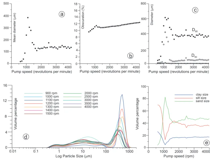
Results of the P1-test of sub-sample aliquot CABRE3b are

(6)

0 1000 2000 3000 4000 0

500

Mean diameter (

m

m)

0 1000 2000 3000 4000

0 200 400 600 800

Pump speed (revolutions per minute) D50

D90

a

Obscuration (%)

0 1000 2000 3000 4000

0 2 4 6 8 10 12 14 16 18

b

Diameter (

m

m)

c

400

300

200

100

0.01 0.1 1 10 100 1000

900 rpm

V

olume percent

age

8 12 16

4

0

V

olume percent

age

Pump speed (rpm)

d

e

0 1000 2000 3000 4000

0 20 40 60 80 100

Fig. 5. Results of the pump speed test P1performed on sub-sample aliquot CABRE3b by the Hydro 2000 MU dispersion unit. (a)Mean

diameter value evolution with increasing the pump speed from 600 up to 4000 rpm.(b)Laser obscuration value progression during the same test.(c)Progression ofD₁₀,D₅₀, andD₉₀percentiles during the same test.(d)Granulometric curves obtained by averaging data from the corresponding 10 measurement runs during representative pump speed steps.(e)Distribution of clay, silt, and sand size fractions during the test.

A comparative P5-test of sub-sample aliquot CABRE3c

was performed with the Hydro 2000 S dispersion unit. The overall behaviour is quite similar to the previous test, with very low mean diameter values at 500 rpm, a maximum at 1200 rpm, and a decrease up to 2000 rpm. The last steps, with pump speed increments of 500 rpm, show quite small variations (Fig. 6a). A P5-test by the Hydro 2000 S

dis-persion unit of sub-sample aliquot SAND1b, from 500 to 2500 rpm, shows a bell-shaped distribution of mean diameter values similar to that produced by using the Hydro 2000 MU dispersion unit (Fig. 6b). Comparison of pump speed test re-sults from sample CABRE, acquired at 5 s of measurement run time by the Hydro 2000 MU and S dispersion units, shows that the former systematically provides higher mean diameter values at low pump speed ranges up to 1100 rpm, including the highest one (Fig. 6c). In the 1200 to 1600 rpm range, higher mean diameter values are provided by the Hy-dro 2000 S unit. At higher pump speed, values provided by the two dispersion units are similar.

Interpretation of the pump speed test results

(7)

eolian sand carbonate breccia

400 800 1200 1600 2000

0 100 200 300 400 500

Mean diameter (

m

m)

Pump speed (revolutions per minute) Hydro S

Hydro MU 0

500

0 1000 2000 3000 4000

a

400

300

200

100

0 500 1000 1500 2000 2500

0 500

b

400

300

200

100

Mean diameter

(

m

m)

Mean diameter

(

m

m)

c

Fig. 6. (a)Pump speed test P5performed on sub-sample aliquot

CABRE3c by the Hydro 2000 S dispersion unit; mean diame-ter value evolution with increasing the pump speed from 500 up to 3500 rpm. (b) Pump speed test P5 performed on sub-sample

aliquot SAND1b by the Hydro 2000 S dispersion unit; mean di-ameter value evolution with increasing the pump speed from 500 up to 2500 rpm.(c)Comparison, in the range 500–2000 rpm, of the trends of mean diameter values obtained from pump speed tests on sample CABRE. The solid line refers to data in Fig. 3a; the broken line refers to data in Fig. 6a.

Mean diameter (

m

m)

fineward bias

coarseward

bias

negligible size reduction

significant size reduction

IV

III

II

I

Fig. 7.Conceptual sketch showing the four main stages character-ising the typical asymmetric bell shaped curve resulting from the progression of mean diameter values during pump speed tests of granular materials. See text for details.

2100 rpm, whereas obscuration remains almost constant and within the initial reference interval from 1500 to 2000 rpm (Fig. 4b). This evidence suggests that highest mean diameter values are coarseward biased through inefficient sample re-circulation, and that values in the plateau characterizing both mean diameter and laser obscuration values, correspond to the most likely measurement runs. In CABRE3b the obscu-ration data point plateau adjacent to the maximum value is not well developed and, conversely, it seems to indicate a slight increase of finer material during measurement. How-ever, analysis of theD10,D50, andD90percentiles does not

indicate significant particle size reduction despite significant scattering.

(8)

measurement run number

a

e

b

c

0 20 40 60 80 100

measure run number

d

0.01 0.1 1 10 100 1000

6 12 18

0

V

olume percent

age

sand size

0 20 40 60 80 100

Linear Fit:

Y = 0.001588220822 * X + 271.6571448 Average Y = 271.737

Residual sum of squares = 84.7112 Regression sum of squares = 0.210183 R-squared = 0.00247503

0 100 200 300 400 500

0 20 40 60 80 100

0 200 400 600 800

D50

D90

D10

Mean diameter (mm)

Volume percentage

Obscuration (%) Diameter (mm)

16

14

10

8

4

2 Measurement run number

Mode (

m

m)

0 2 4 6 8 10

250 260 270 280 curve 1

curve 100 curve 90 curve 80 curve 70 curve 60 curve 40 curve 30 curve 20 curve 10

curve 50

0 20 40 60 80 100

10 11 12 13 14

Linear fit:

Y = -0.01827272727 * X + 262.8133636 Average Y = 262.704

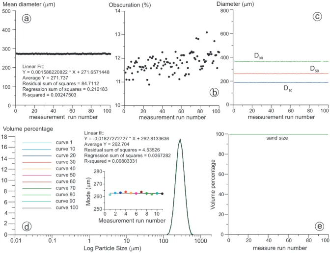
Fig. 8.Results of the measurement precision test MP25005performed on sub-sample aliquot SAND1c by the Hydro 2000 MU dispersion

unit.(a)Mean diameter value evolution with increasing the number of measurement runs. Data statistics are provided.(b)Laser obscuration value progression during the same test. (c)Progression ofD₁₀,D₅₀, andD₉₀percentiles during the same test. (d)Granulometric curves representative of the particle size evolution. Note their virtually perfect overlap. The corresponding modal values (same colour code) are illustrated in the inset graph, whose statistics are also provided. Note how average modal and mean values are very similar.(e)Distribution of the sand size fractions during the test. It represents 100% of the sample, without any significant amount of clay and silt.

Results from the pump speed tests illustrated above can be schematically explained by a composite trend of mean values as a function of pump speed values, where four major stages can be identified (Fig. 7): (1) an initial segment characterized by very low mean diameter values, which is interpreted to in-dicate fineward bias by ineffective material recirculation into the dispersion unit and measurement cell; (2) the adjacent, bell-shaped segment containing the maximum mean diame-ter values, which is indiame-terpreted to indicate coarseward bias by ineffective material recirculation; (3) the third, flat-lying or slowly dipping segment, which is interpreted to indicate effective material recirculation without significant mechani-cal alteration, thus providing the most effective pump speed size range for further analyses; (4) the fourth segment, char-acterised by progressively decreasing mean diameter values indicating the occurrence of significant mechanical alteration and consequent fineward biasing of the sample material data.

The geometry of this last segment might be also influenced by a differential velocity between coarse and fine particles: being the recirculation of the latter faster, this might create the illusion of a higher content of fines.

5 Measurement precision test

Results from the pump speed test on the SAND1 sample in-dicate negligible influence of this parameter for values higher than 2000 rpm. We performed a MP25005test (i.e. 2500 rpm

of pump speed and 5 s of measurement run time) on sub-sample aliquot SAND1c (Fig. 8). Mean diameter values dis-play only slight variation between the 100 runs, as do the D10,D50, andD90 percentiles, while obscuration values are

(9)

100 measurement run number

a

0 100 200 300 400 500

0 20 40 60 80

Linear Fit:

Y = -0.3149409241 * X + 220.0308467 Average Y = 204.126

Mean diameter (mm)

e

b

12 13 14 15

0 20 40 60 80 100

Linear Fit:

Y = 0.007706450645 * X + 13.77582424

0 20 40 60 80 100

0 200 400 600 800

D10

D50

D90

c

measurement run number measurement run number

0 20 40 60 80 100

d

Log Particle Size (mm) Volume percentage

0.01 0.1 1 10 100 1000

2 4 6

0

V

olume percent

age

curve 100

1 10 50 100

360 380 400 420 440 460 480 500

Mode (

m

m)

Measurement run number curve 1

curve 90 curve 80 curve 70 curve 60 curve 40 curve 30 curve 20 curve 10

curve 50

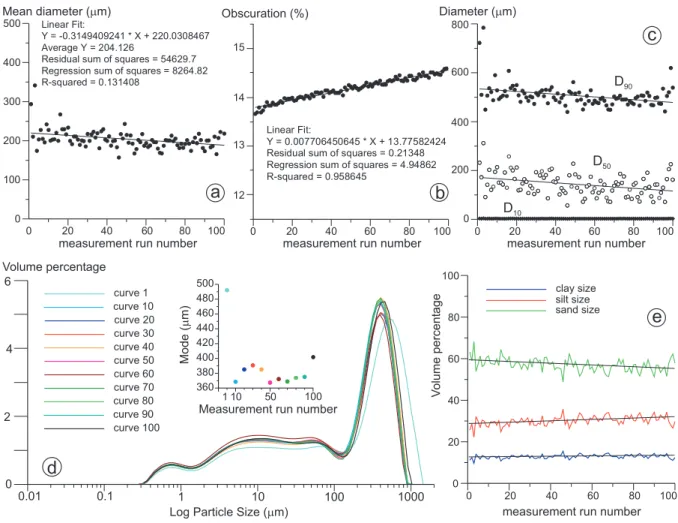
Fig. 9.Results of the measurement precision test MP2000₅performed on sub-sample aliquot CABRE3d by the Hydro 2000 MU dispersion unit.(a)Mean diameter value evolution with increasing the number of measurement runs. Data statistics are provided.(b)Laser obscuration value progression during the same test. Data statistics are provided.(c)Progression ofD₁₀,D₅₀, andD₉₀percentiles during the same test. (d)Granulometric curves representative of the particle size evolution. The corresponding modal values (same colour code) are illustrated in the inset graph.(e)Distribution of the clay, silt and sand size fractions during the test.

the corresponding mode values (Fig. 8d). This indicates that no material finer than sand was produced during measure-ment runs (Fig. 8e).

The pump speed test for sample CABRE3 indicates that 2000 rpm is the most suitable pump speed value to ensure ef-fective material recirculation without very invasive mechan-ical alteration. Moreover, 5 s of measurement run time are expected to provide more statistically robust results than 1 s. Accordingly, we initially performed a MP20005, test on

sub-sample aliquot CABRE3d (Fig. 9). Mean diameter values show significant scattering and a slightly decreasing trend with time, while laser obscuration progressively increased. The value ofD50, andD90percentiles show a pattern

simi-lar to the mean diameter, being the scattering of the former particularly higher. On the other hand,D10 percentile

val-ues are extremely small. Selected granulometric curves are quite similar apart from the first run (Fig. 9d). The corre-sponding modal values show a much higher mode for the

first run, followed by a drop of about 140 µm in the sec-ond one. Slightly higher values characterize runs 3 to 5, and then very similar values pertain to the following runs (about 350 µm) with the exception of the last one, which has a higher mode, slightly higher than 400 µm. The distribution of sand, silt and clay size fractions shows a scattered pattern about a slightly decreasing trend for the sand size, less scattering about a slightly increasing trend for the silt size, and negli-gible scattering with near constant values for the clay size fraction (Fig. 9e).

(10)

a

Linear Fit:

Y = 0.1612023402 * X + 422.9113418 Average Y = 431.052

0 100 200 300 400 500

0 20 40 60 80 100

Mean diameter (

m

m)

f

0 20 40 60 80 100

Linear Fit:

Y = -0.3405654845 * X + 197.785317 Average Y = 180.587

d

Obscuration (%)

b

0 20 40 60 80 100 12

13 14 15

Linear Fit

Y = -0.002659105911 * X + 14.45768485 Residual sum of squares = 19.5907 Regression sum of squares = 0.589178 R-squared = 0.0291964

0 20 40 60 80 100 0

200 400 600 800

D₉₀

D₅₀

D10

measure run number

c

Diameter (

m

m)

measure run number measure run number

0 20 40 60 80 100 12

13 14 15

Linear Fit:

Y = 0.01323192319 * X + 14.37078788

e

Obscuration (%)

0 20 40 60 80 100 0

200 400 600 800

measure run number

i

D90

D50

D10

Diameter (

m

m)

1200 rpm

4000 rpm

0 100 200 300 400 500

Mean diameter (

m

m)

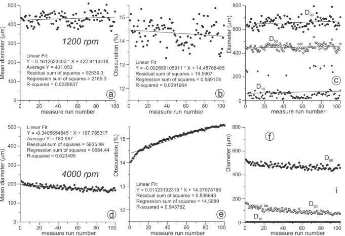
Fig. 10.Comparison between measurement precision test results performed on sample CABRE3 at the pump speed velocity corresponding to the mean diameter peak value of the pump speed test (Fig. 3a), and at the maximum pump speed, respectively.(a)Test MP12005performed

on sub-sample aliquot CABRE3e by the Hydro 2000 MU dispersion unit; mean diameter value evolution with increasing the number of measurement runs. Data statistics are provided. (b)Laser obscuration value progression during the same test. Data statistics are provided. (c)Progression ofD₁₀,D₅₀, andD₉₀percentiles during the same test.(d)Test MP40005performed on sub-sample aliquot CABRE3f by

the Hydro 2000 MU dispersion unit; mean diameter value evolution with increasing the number of measurement runs. Data statistics are provided.(e)Laser obscuration value progression during the same test. Data statistics are provided.(f)Progression ofD₁₀,D₅₀, andD₉₀

percentiles during the same test. Note the very large difference between the average mean diameter obtained from the first (431.052 µm) and the second test (180.587 µm), respectively. Both them are affected by strong recirculation-related mechanical bias.

tests designed to investigate the influence of measurement run time were performed at 2000 rpm pump speed and 1 s, 10 s, 20 s, and 40 s of measurement run time, respec-tively. The MP20001, test on sub-sample aliquot CABRE3g

(Fig. 11) is characterised by intense scattering of mean diam-eter values that show an increasing trend with increasing the run number (i.e. time). Intense scattering also occurs inD50,

andD90 percentiles and in the sand, silt and clay size

frac-tion data. The selected granulometric curves show a higher variability and a non systematic trend, compared to the cor-responding ones acquired at 5 s of measurement run time, as also indicated by the corresponding modal values (Fig. 11d). For a constant total duration of the measurement precision test, increasing the measurement run time causes a decrease of mean diameter data scattering and more linearly increas-ing trends of laser obscuration values (Fig. 12). We also ran a MP5test on sub-sample aliquot CABRE3k by using the Cilas

930 laser diffraction particle size analyser. Results provided significantly smaller mean diameter values with respect to those provided by the Mastersizer 2000, and these values sys-tematically decreased through time, as indicated by the very good linear best fit (Fig. 13).

Plotting mean diameters of test MP20005averaged every

(11)

100

measure run number

a

0 100 200 300 400 500

0 20 40 60 80

Mean diameter (mm)

e

b

9 10 11 12

0 20 40 60 80 100 0 20 40 60 80 100

0 200 400 600 800

D10 D50

c

0 20 40 60 80 100

measure run number

d

0.01 0.1 1 10 100 1000

2 4 6

0

V

olume percent

age

clay size silt size sand size curve 1

curve 100 curve 90 curve 80 curve 70 curve 60 curve 40 curve 30 curve 20 curve 10

curve 50

D90

8

Linear fit:

Y = 0.008490069007 * X + 10.48195152 Residual sum of squares = 0.655079 Regression sum of squares = 6.00617 R-squared = 0.901658

1 10 50 100

300 340 380 420 460 500

Measurement run number

Mode (

m

m)

Regression sum of squares = 41648 R-squared = 0.225649

Linear fit:

Y = 0.7069838524 * X + 193.5241855 Average Y = 229.227

Residual sum of squares = 142922

Fig. 11.Results of the measurement precision test MP20001performed on sub-sample aliquot CABRE3g by the Hydro 2000 MU dispersion

unit.(a)Mean diameter value evolution with increasing the number of measurement runs. Data statistics are provided.(b)Laser obscuration value progression during the same test. Data statistics are provided.(c)Progression ofD₁₀,D₅₀, andD₉₀percentiles during the same test. (d)Granulometric curves representative of the particle size evolution. The corresponding modal values (same colour code) are illustrated in the inset graph.(e)Distribution of the clay, silt and sand size fractions during the test.

are quite similar and have a modal peak of about 400 µm that remains unchanged also after 50 and 100 runs (Fig. 14d). In particular, the third run curve provides the coarsest distribu-tion, and the correspondingD10, D50, andD90 percentiles

and modal value are outliers with respect to the overall trend of the other data (Fig. 14e–g). This evidence questions the validity of the third run data.

Interpretation of the measurement precision test results

The measurement precision test provided contrasting results depending on the rock type. Carbonate cataclastic breccias are sensitive to the material recirculation time (i.e. the num-ber of measurement runs and/or the measurement run time), whereas eolian sand data remains almost unaltered through time. In particular, in carbonate cataclastic breccias a signifi-cant difference occurs between the first run and the following

ones, suggesting that only short recirculation times ensure a small mechanical bias to particle size data from wet suspen-sion analyses.

6 Ultrasonication test

An ultrasonication test on eolian sand was performed on sub-sample aliquot SAND1d, using the maximum ultrasonication probe tip displacement (20 µm), 2500 rpm of pump speed, and 5 s of measurement run time (US205). Mean diameters

(12)

0 10 20 30 40 50 0

100 200 300 400

500 Linear Fit:

Y = -0.4961758944 * X + 206.8466653 Average Y = 194.194

0 10 20 30 40 50

13 14 15 16 17 18

Obscuration (%)

0 5 10 15 20 25

0

500 Linear Fit:

Y = -0.4750692308 * X + 176.2197 Average Y = 170.044

0 5 10 15 20 25

11 12 13 14 15 16

0 1 2 3 4 5 6 7 8 9 10 11 12 13

0

500 Linear Fit:

Y = -1.851313187 * X + 200.3955769 Average Y = 187.436

0 1 2 3 4 5 6 7 8 9 10 1112 13 10

11 12 13 14 15

c

d

a

b

f

e

measurement run time = 10s

Mean diameter (

m

m)

measurement run time = 20s measurement run time = 40s

measure run number measure run number measure run number

Fig. 12.Results of measurement precision tests performed at different run times on sample CABRE3 by the Hydro 2000 MU dispersion unit. (a)Test MP2000₁₀on sub-sample aliquot CABRE3h; mean diameter value evolution with increasing the number of measurement runs. Data statistics are provided.(b)Laser obscuration value progression during the same test.(c)Test MP200020on sub-sample aliquot CABRE3i;

mean diameter value evolution with increasing the number of measurement runs. Data statistics are provided. (d)Laser obscuration value progression during the same test. (e)Test MP200040on sub-sample aliquot CABRE3j; mean diameter value evolution with increasing the

number of measurement runs. Data statistics are provided.(f)Laser obscuration value progression during the same test.

about 259 µm. The corresponding volume percentage drops of about 1.75% from curve 7 onward (Fig. 15c). Modal val-ues remain almost constant for the entire test, about an aver-age value of 258.5 µm (Fig. 15d). Contrasting these 10 curves from the ultrasonication test, against the first one from the measurement precision test on sub-sample aliquot SAND1c indicates negligible differences (Fig. 15c).

Ultrasonication intensities of 2.5 µm, 5 µm, 10 µm, and 20 µm of tip displacement were applied to the carbonate cat-aclastic breccia, using a pump speed of 2000 rpm and 5 s of measurement run time. Results indicate that increasing the ultrasound energy causes (i) a faster decrease of mean diam-eter values, which passes from linear to power law best fit curves, (ii) higher increases of laser obscuration, and (iii) a decrease of average modal values up to 10 µm, which remain almost constant when the maximum probe tip displacement is used (Fig. 16). Analysis of granulometric curves pertain-ing to the first 10 runs and to runs 50 and 100 in each test shows a progressively increasing difference between first run curves and the remaining ones with increasing the

ultrason-ication probe tip displacement (Fig. 17). Moreover, shape differences among curves increase, particularly between test US2.55and the remaining ones, and the modal peak volume

percentage of the bulk of the curves in each test decreases with increasing ultrasonication intensity. Comparison of the first run curves from tests with and without ultrasonication shows that the latter provide a significantly coarser particle size distribution in the modal peak (Fig. 17e). The influ-ence of ultrasonication is also illustrated by the differinflu-ence between first-run modal values and those averaged over the first 10 runs of the corresponding tests. The greater differ-ence occurs when no ultrasonication was used. The smaller difference occurs at the minimum ultrasonication intensity and then it increases up to the US105test.

Interpretation of the ultrasonication test results

(13)

0 100 200 300 400 500

0

measure number

10 20 30

174.63 mm

151.69 mm

136.69 mm

132.60 mm

Mean diameter (

m

m)

Linear Fit:

Y = -1.413119021 * X + 166.5176782 Average Y = 144.614

Fig. 13.Results of a measurement precision tests performed on sub-sample aliquot CABRE3k by the Cilas 930 laser diffraction particle size analyser; mean diameter value evolution with increasing the number of measurement runs. Data statistics are provided.

test evidence. On the other hand, in the carbonate cataclas-tic breccia sub-sample aliquots, ultrasonication has a much greater influence causing significant particle size reductions after few measurement runs, as indicated by the concomi-tant reduction of mean diameter and mode values, by the in-crease of laser obscuration, and by the inin-crease of volume percentages in the 0.5 µm to 100 µm segments of granulo-metric curves. Even after a single measurement run, ultra-sonication is able to shift fineward the modal peak value of particle size distributions by 60 to 80 µm.

7 Chemical test

In wet analyses, liquid dispersants can wet microfractures and help cohesion loss, thus favouring disintegration of mi-crofractured particles. Fracture aperture thresholds for capil-larity permeability depend on the surface tension of the dis-persant liquid. Accordingly, disdis-persant liquids with low sur-face tensions are expected to enhance particle disintegration in cataclastic materials, whereas this effect should be negli-gible for intact particles. To test this hypothesis, denaturated ethyl alcohol was used as dispersant liquid for data acqui-sition from eolian sand by performing a MP25005al, test on

sub-sample aliquot SAND1e. Results are very consistent, as illustrated by the almost constant mean diameter values, by the flat lying best fit line of mode values, and by the very sim-ilar granulometric curves in the first 10 runs, which provide an extremely good overlap with the first curve from the same test using decalcified tap water as dispersant liquid (Fig. 18).

The corresponding modal values show an initial decrease of less than 5 µm, reaching a plateau value after 4 runs.

Two measurement precision test were performed on CABRE3p and CABRE3q sub-sample aliquots, using denat-urated ethyl alcohol and demineralised water, respectively (Fig. 19). The first test provided quite scattered mean diam-eter and mode values, both characterized by flat-lying best fit lines, which are smaller than the corresponding ones ob-tained from demineralised water of about 70 µm and 53 µm, respectively. The increase of laser obscuration values is greater for the dispersion in denaturated ethyl alcohol. Anal-ysis of granulometric curves pertaining to the first 10 runs in-dicates a higher variability for measurements acquired in de-naturated ethyl alcohol, of both curve shape and modal peak elevation (Fig. 19g, h). Such a higher variability is confirmed by the analysis of the corresponding modal values. Finally, comparison with the first run curve from the same test using decalcified tap water as dispersant liquid, indicates that gran-ulometric curves obtained from the denaturated ethyl alcohol suspension have much greater differences with respect to the corresponding ones acquired using demineralised water as dispersant liquid.

Interpretation of the chemical test results

Test results indicate that the use of denaturated ethyl alcohol has a negligible influence on data acquisition in quartz eolian sand. Variations of mean diameter and mode values are less than 5 µm, which fall inside the variability associated with sub-sampling, even in well sorted sediments like dune sands. On the other hand, the same dispersant liquid causes a de-crease of about 75 µm of mean diameter values when car-bonate cataclastic breccia is analysed. The evidence that, when demineralised water is used, results are very similar to those from the corresponding test in decalcified tap water rules out any significant bias produced by sub-sampling and supports particle fragmentation during suspension recircula-tion. This is well illustrated by the systematic decrease of modal peak volumes and size, and by the corresponding in-crease of volume percentage values in the 0.5 µm to 110 µm segments of granulometric curves in Fig. 19g. Higher varia-tions occurs after only two runs. It is worth noting that many other dispersants could be used, as well as various pretreat-ments. However, performing detailed investigations on this is out of our purposes in this paper.

8 Reprocessing test

The first run of the MP25005test was selected for data

(14)

Diameter (

m

m)

D50

D90

0 4 8 10

0 200 400 600 800

6

2 50

100

0 2 4 6 8 10 50

100

Diameter (

m

m) Measurement number

D₁₀

200 210 220 230 240 250

Mean diameter (

m

m)

analysis time (s)

0 100 200 300 400 500

13.6 13.8 14 14.2 14.4

Measurement number

6 8 50

100

4 2

Measure n.

Obscuration (%)

f

0.01 0.1 1 10 100 1000

2 4 6

0

curve 1

curve 6

curve 50 curve 100

2.5 3 3.5 4 4.5

a

b

e

d

350 370 380 390 400 410

Mode (

m

m)

analysis time (s)

0 100 200 300 400 500

360

0 2 4 6 8 10

320 360 400 440 480 520

Mode (

m

m)

100

50

g

c

Fig. 14. Analysis of data from the test MP20005on -sample aliquot CABRE3d (Fig. 9). (a)Mean diameter values averaged every five

measurement runs.(b)Average modal values corresponding to data in (a). In both cases, the best fits indicate an exponential decay.(c)Laser obscuration values recorded during the first 10 runs (black dots), compared with the values after 50 (red dot) and 100 (blue dot) measurement runs. (d)Granulometric curves computed for the first 10 runs, compared with the ones from the 50th and 100th run. (e)Progression of

D₅₀andD₉₀percentiles during the first 10 measurement runs. Data after 50 (red dot) and 100 (blue dot) runs are provided for comparison. (f)Progression ofD₁₀ percentiles during the first 10 measurement runs. Data after 50 (red dot) and 100 (blue dot) runs are provided for comparison.(g)Progression of modal values during the first 10 measurement runs (colour code as in (d)). Data after 50 (grey dot) and 100 (black dot) runs are provided for comparison.

values show a very small variability. The same result was ob-tained when varying ABS values from 1.00 to 0.01 (Fig. 21). Changing RI in carbonate cataclastic breccia (first run of test MP20005 on sub-sample aliquot CABRE3d) causes some

variability in the corresponding grain size distributions, par-ticularly from RI = 1.4 to RI = 1.6 (Fig. 22). Analysis of residuals associated with best fit curves indicates that the most appropriate RI value is 1.6. Higher values, however,

(15)

0 20 40 60 80 100 0

100 200 300 400 500

24 25 26 27 28 29 30 31 32 33 34 35 36 37

Mean diameter (

m

m)

measure number

Linear fit:

Y = -0.1183510451 * X + 270.4132088 Average Y = 264.496

0 20 40 60 80 100

measure number

Obscuration (%)

a

b

measure number Log Particle Size (mm)

1 10 100 1000

0.1

c

V

olume percent

age

4 12 16

0 8

Linear fit on the first 26 runs Y = 0.0142817094 * X + 270.6178892 Average Y = 270.811

R-squared = 0.00286513

Linear fit on the remaining 73 data Y = -0.04511039121 * X + 263.9155502 Average Y = 262.246

R-squared = 0.315638

0 20 40 60 80 100

250 260 270 280 curve 1

curve 6

curve 1 no US

Mode (

m

m)

Linear fit:

Y = -0.005597897341 * X + 258.790905 Average Y = 258.511

d

Fig. 15. Results of the ultrasonication test US205performed on sub-sample aliquot SAND1d by the Hydro 2000 MU dispersion unit. (a)

Mean diameter value evolution with increasing the number of measurement runs. Data statistics are provided for the cumulative dataset, for the first 26 runs, and for the remaining 73 runs, respectively.(b)Laser obscuration value progression during the same test.(c)Granulometric curves computed for the first 10 runs, compared with the first curve from the test MP25005 on sub-sample aliquot SAND1c (Fig. 8).

Progression of modal values with increasing the number of measurement runs. Data statistics are provided.

values and a decrease of modal values. Analysis of resid-uals associated with best fit curves indicates that the most appropriate ABS value is 0.01. Finally, changing the RI val-ues of the dispersant liquid has negligible effects on eolian quartz sand, and an influence on CABRE material that is comparable to what is produced by changing RI of carbonate particles (Fig. 24).

Interpretation of reprocessing test results

Results of these tests indicate that in the case of the analyzed materials, the sensitivity of light scattering data reprocess-ing by the Mie theory is mainly governed by the particle size range, rather than by their optical properties. In fact, the very good sorting of sample SAND1 results in a virtually insen-sitive behaviour to reprocessing, while the large spanning of

sizes in CABRE3 enhances the sensitivity of particles finer that about 2 µm.

9 Discussion

(16)

c

0 20 40 60 80 100 0

500

Power Law Fit

Y = pow(X,-0.1033986354) * 226.463531 Residual sum of squares = 1.15809 Regression sum of squares = 0.911613 R-squared = 0.440456

d

measure number US = 5.0 _mm

100 200 300 400 a 0 100 200 300 400 500

0 20 40 60 80

Linear Fit:

Y = -0.1899744374 * X + 182.4314691 Average Y = 172.838

Residual sum of squares = 32919 Regression sum of squares = 3007.22 R-squared = 0.0837055

Mean diameter (

m

m)

100

measure number

Obscuration (%)

0 20 40 60 80 100 10

12 14

16

18 Power Law Fit:

Y = pow(X,0.04232472628) * 10.8680306 Residual sum of squares = 0.000679821 Regression sum of squares = 0.152746 R-squared = 0.995569

Sigma-hat-sq'd = 6.93695E-006

b

Mean diameter (

m

m)

measure number

0 20 40 60 80 100 10

12 14 16

18 _{Power Law Fit:}

e

Obscuration (%)

measure number

g

0 20 40 60 80 100

Power Law Fit:

0 100 200 300 400 500

Mean diameter (

m

m)

US = 10.0 _mm

0 500

0 20 40 60 80 100

Power Law Fit:

l

10 12 14 16 measure number 18

0 20 40 60 80 100

Power Law Fit:

h Obscuration (%) 10 12 14 16 18

0 20 40 60 80 100

Power Law Fit

m measure number Obscuration (%) 100 200 300 400

Mean diameter (

m m) 200 300 400 500 600

0 20 40 60 80 100

measure number Mode ( m m) n Linear fit:

Y = -0.1322146715 * X + 348.4902909 Average Y = 341.813

200 300 400 500 600

0 20 40 60 80 100

measure number Mode ( m m) i 200 300 400 500 600

0 20 40 60 80 100

measure number Mode ( m m) f 200 300 400 500 600

0 20 40 60 80 100

measure number

Mode (

m

m)

Linear fit:

Y = -0.1255660546 * X + 358.9963158 Average Y = 352.655

Linear fit:

Y = -0.1172544734 * X + 370.2030109 Average Y = 364.282

Linear fit:

Y = -0.2282990159 * X + 353.2929703 Average Y = 341.764

Fig. 16. Ultrasonication tests on sample CABRE3 by the Hydro 2000 MU dispersion unit. (a)Ultrasonication test US2.55performed on

sub-sample aliquot CABRE3l; mean diameter value evolution with increasing the number of measurement runs.(b)Laser obscuration value progression during the same test.(c)Mode value progression during the same test.(d)Ultrasonication test US5₅performed on sub-sample aliquot CABRE3m; mean diameter value evolution with increasing the number of measurement runs.(e)Laser obscuration value progression during the same test. (f)Mode value progression during the same test. (g)Ultrasonication test US10₅performed on sub-sample aliquot CABRE3n; mean diameter value evolution with increasing the number of measurement runs.(h)Laser obscuration value progression during the same test.(i)Mode value progression during the same test.(l)Ultrasonication test US205performed on sub-sample aliquot CABRE3o;

(17)

Volume percentage

1 10 100 1000

0.1

curve 50 curve 100 curve 1

curve 6

2 4 6

0

d

US = 20 _mm

Volume percentage

1 10 100 1000

0.1

curve 6

2 4 6

0

a

US = 2.5 _mm

Volume percentage

1 10 100 1000

0.1

curve 6

2 4 6

0

b

US = 5 _mm

Volume percentage

1 10 100 1000

0.1

curve 6

2 4 6

0

c

US = 10 _mm

V

olume percent

age

1 10 100 1000

0.1

e

no US 460 500

420

380

340

300

US 2.5

US 5

US 10

US 20

US = 20 mm

US = 10 mm US = 5 mm

US = 2.5 mm

no US

Mode (

m

m)

0 2 4 6

Fig. 17. (a)Granulometric curves computed for the first 10 runs of test US2.55performed on sub-sample aliquot CABRE3l, compared with

the ones from the 50th and 100th run.(b)Granulometric curves computed for the first 10 runs of test US55performed on sub-sample aliquot

CABRE3m, compared with the ones from the 50th and 100th run. (c)Granulometric curves computed for the first 10 runs of test US10₅ performed on sub-sample aliquot CABRE3n, compared with the ones from the 50th and 100th run. (d)Granulometric curves computed for the first 10 runs of test US20₅performed on sub-sample aliquot CABRE3o, compared with the ones from the 50th and 100th run. (e) First run granulometric curves from the four tests listed above, compared with the first run curve from test MP20005on sub-sample aliquot

(18)

1 2 3 4 5 6 7 8 9 10 250

260 270

Mode (

m

m)

c

a

Mean diameter (

m

m)

measurement run number measurement run number

Obscuration (%)

b

0 20 40 60 80 100

Mode (

m

m)

0 20 40 60 80 100

0 100 200 300 400 500

Linear Fit:

Y = 0.0009950435043 * X + 267.9889503 Average Y = 268.039

Sigma-hat-sq'd = 1.24454

0 20 40 60 80 100

10 11 12 13 14

250 260 270 280 290 300

Linear fit:

Y = 0.002526540654 * X + 257.6840297 Average Y = 257.812

Average Y = 258.715

e

1 10 100 1000

0.1

V

olume percent

age

4 12 16

0 8

curve 1

curve 6

curve 1 tap water 2

6 10 14 18

d

Fig. 18.Results of the chemical test MP25005alperformed on sub-sample aliquot SAND1e by the Hydro 2000 MU dispersion unit, using

denaturated ethyl alcohol as dispersant liquid. (a)Mean diameter value evolution with increasing the number of measurement runs. Data statistics is provided. (b)Laser obscuration value progression during the same test. (c)Progression of modal values with increasing the number of measurement runs. Data statistics are provided.(d)Granulometric curves computed for the first 10 runs, compared with the first curve from the test MP2500₅on sub-sample aliquot SAND1c (Fig. 8).(e)Modal values corresponding to the curves in (d).

In fact, in this case particles are produced by multiple frac-turing, rolling and grinding of material within fault zones (e.g. Borg et al., 1960; Storti et al., 2003; Sammis and Ben Zion, 2008). Particle size depends on the relative strength distribution along cleavage and microfracture sets as a func-tion of the applied stress (e.g. Sammis et al., 1987). Ac-cordingly, the mechanical behaviour of these carbonate cat-aclastic particles can be compared to that of sedimentary particles made of cohesive aggregate grains. Conversely, multiple collisions of quartz particles during eolian trans-port along coastal dunes ensures effective exploiting of pre-existing flaws. The resulting rounded particles are strong enough for being not significantly influenced by mechanical solicitations in laser diffraction particle size analysers.

It follows that determining the appropriate operating pro-cedure bears a fundamental importance for heavily mi-crofractured materials, while it has secondary effect when high strength particles are analysed. In the latter case, only pump speed can influence the final results by not ensuring effective particle recirculation in the dispersion unit. How-ever, given the high strength of this material, pump speed

(19)

a

b

Mean diameter (mm) Obscuration (%)

0 20 40 60 80 100 0

100 200 300 400 500

Linear Fit:

Y = 0.05530309631 * X + 126.6512636 Average Y = 129.444

Power Law Fit:

d

Mean diameter (mm) Obscuration (%)

0 20 40 60 80 100 0

100 200 300 400 500

0 20 40 60 80 100 Linear Fit:

Y = 0.1002275308 * X + 195.6247497 Average Y = 200.686

10 11 12 13 14

e

0 20 40 60 80 100 13

14 15 16 17

Power Law Fit:

Mode (mm)

0 20 40 60 80 100 0

100 200 300 400 500

Linear fit:

Equation Y = -0.02004089409 * X + 331.61 Average Y = 330.608

c

Mode (mm)

0 20 40 60 80 100 0

100 200 300 400 500

f

Linear fit:

Equation Y = 0.03191116112 * X + 382.176 Average Y = 383.788

denaturated ethylic alcohol

demineralised water

Volume percentage

1 10 100 1000

0.1 2

4 6

0

Volume percentage

1 10 100 1000

0.1 2

4 6

0

curve 1 tap water curve 1

curve 6

g

0 2 4 6 8 10 250

300 350 400 450

Mode (

m

m)

h

Fig. 19.Results of chemical tests performed on sample CABRE3e by the Hydro 2000 MU dispersion unit. (a)Test MP20005alperformed

on sub-sample aliquot CABRE3p using denaturated ethyl alcohol as dispersant liquid; mean diameter value evolution with increasing the number of measurement runs. Data statistics are provided. (b)Laser obscuration value progression during the same test. Data statistics are provided. (c)Progression of modal values with increasing the number of measurement runs. Data statistics are provided. (d)Test MP20005dwperformed on sub-sample aliquot CABRE3q using demineralised water as dispersant liquid; mean diameter value evolution

with increasing the number of measurement runs. Data statistics are provided.(e)Laser obscuration value progression during the same test. Data statistics are provided.(f)Progression of modal values with increasing the number of measurement runs. Data statistics are provided. (g)Granulometric curves computed for the first 10 runs in (a), compared with the first curve from the test MP20005on sub-sample aliquot

CABRE3d (Fig. 9).(h)Granulometric curves computed for the first 10 runs in (d), compared with the first curve from the test MP20005on

(20)

a

1 10 100 1000

0.1

RI = 1.4

RI = 1.8 RI = 1.7 RI = 1.6 RI = 1.5

6 12 18

0 1 4 8 12 16 20 24 28 32 36 40 44 48 52 4000

3000

2000

1000

0

1 4 8 12 16 20 24 28 32 36 40 44 48 52 4000

3000

2000

1000

0

Detector number Detector number

Light energy

1 4 8 12 16 20 24 28 32 36 40 44 48 52 4000

3000

2000

1000

0

1 4 8 12 16 20 24 28 32 36 40 44 48 52 4000

3000

2000

1000

0

Light energy

1.4 366 367 368 370

1.5 1.6 1.7 1.8 Refractive index 365

1.4 261 262 263 265

1 4 8 12 16 20 24 28 32 36 40 44 48 52 4000

3000

2000

1000

0

Detector number

Light energy

1.4 262 263 264 265

260 1.4

189 190

1.5 1.6 1.7 1.8

D90

(

m

m)

Mode

(

m

m)

b

c

d

e

f

16

14

10

8

4

2

188

187

186

185

Refractive index

369 264

D10

(

m

m)

D50

(

m

m)

Fig. 20. Reprocessing of the first run data from test MP25005on sub-sample aliquot SAND1c (Fig. 8). (a)Light scattering data (black

curve) and corresponding best fits for variable RI values of quartz from 1.4 to 1.8 (colour code in (b)), constant ABS values of quartz = 0.1, and constant RI values of decalcified tap water = 1.33.(b)Granulometric curves computed from reprocessed data in (a).(c)D₁₀percentiles for data in the 5 curves illustrated in (b).(d)D₅₀percentiles for data in the 5 curves illustrated in (b).(e)D₉₀percentiles for data in the 5 curves illustrated in (b). (f)Modal values for data in the 5 curves illustrated in (b). It is worth noting that changing RI of quartz produces negligible changes in the reprocessed data.

Finally, it is worth noting that, despite the effectiveness of statistical parameters like mean diameter, percentiles, and others, they cannot replace the use of granulometric curves for comparing results from different tests. This because very similar average values can relate to very different granulo-metric curves (e.g. Selley, 2000).

10 Conclusions

Particle size distributions significantly contribute to the de-scription of many geological processes including sedimenta-tion, rock fragmentation and soil formation. Modern laser diffraction particle size analysers ensure fast data acquisition over a wide size range, coupled with the appropriate

flexibil-ity for analysing very different granular materials. This flex-ibility, however, can produce severely biased results when inappropriate analytical operating procedures are used, par-ticularly on fragile materials. We analysed both high strength (eolian quartz sand) and low strength (carbonate cataclas-tic breccia) essentially monomineralic materials to test the impact of different analytical operating procedures involving particle dispersion into a liquid, on the obtained particle size distributions. Our results can be summarised by the follow-ing points:

(21)

a

1 10 100 1000

0.1 6 12 18

0 1 4 8 12 16 20 24 28 32 36 40 44 48 52 4000

3000

2000

1000

0

1 4 8 12 16 20 24 28 32 36 40 44 48 52 4000

3000

2000

1000

0

Light energy

1 4 8 12 16 20 24 28 32 36 40 44 48 52 4000

3000

2000

1000

0

1 4 8 12 16 20 24 28 32 36 40 44 48 52 4000

3000

2000

1000

0

Light energy

366 367 369 370

365

259 260 262 263

258 1 4 8 12 16 20 24 28 32 36 40 44 48 52

4000

3000

2000

1000

0

Detector number

Light energy

262 263 264 265

261

260 189

190

D90

(

m

m)

Mode

(

m

m)

b

c

d

e

f

16

14

10

8

4

2

188

187

186

185

368 261

ABI = 1.00

ABI = 0.01 ABI = 0.05 ABI = 0.10 ABI = 0.50

1.0 0.5 0.1 0.05 0.01 Particle absorption

1.0 0.5 0.1 0.05 0.01 Particle absorption D10

(

m

m)

D50

(

m

m)

1.0 0.5 0.1 0.05 0.01 Particle absorption

Fig. 21.Reprocessing of the first run data from test MP25005on sub-sample aliquot SAND1c (Fig. 8).(a)Light scattering data (black curve)

and corresponding best fits for constant RI values of quartz = 1.5, variable ABS values of quartz from 0.01 to 1.00 (colour code in (b)), and constant RI values of decalcified tap water = 1.33.(b)Granulometric curves computed from reprocessed data in (a).(c)D₁₀percentiles for data in the 5 curves illustrated in (b).(d)D₅₀percentiles for data in the 5 curves illustrated in (b).(e)D₉₀percentiles for data in the 5 curves illustrated in (b). (f)Modal values for data in the 5 curves illustrated in (b). It is worth noting that changing also ABS of quartz produces negligible changes in the reprocessed data.

ineffective pumping and stirring allow particle sedimen-tation; (ii) overestimating coarser particles when in-effective pumping and stirring allow transient particle stagnation within the measurement cell; (iii) underes-timating coarser particles when fast pumping and stir-ring produce significant particle size reduction in low strength material during measurement running;

2. high strength material is not significantly influenced by the adopted instrumentation and standard operating pro-cedure, provided that effective sample recirculation is obtained in the dispersion unit;

3. adding ultrasonication in wet analyses of low strength material systematically causes mechanical particle size

reduction during measurement that, however, is less ef-fective than that caused by fast pumping and stirring during sample recirculation and mainly produces very fine particles by polishing of the larger ones;

4. in low strength material, the number of averaged mea-surement runs has to be carefully determined by statis-tical data analysis of large datasets in order to ensure robust outputs and minimize mechanical biasing of par-ticle size during recirculation in the dispersion unit; 5. Selecting appropriate optical properties for the analysed