BGD
7, 4223–4271, 2010Sensitivity and uncertainty of
ACASA
K. Staudt et al.
Title Page
Abstract Introduction
Conclusions References
Tables Figures
◭ ◮
◭ ◮
Back Close
Full Screen / Esc
Printer-friendly Version Interactive Discussion
Discussion
P
a
per
|
Dis
cussion
P
a
per
|
Discussion
P
a
per
|
Discussio
n
P
a
per
|
Biogeosciences Discuss., 7, 4223–4271, 2010 www.biogeosciences-discuss.net/7/4223/2010/ doi:10.5194/bgd-7-4223-2010
© Author(s) 2010. CC Attribution 3.0 License.
Biogeosciences Discussions
This discussion paper is/has been under review for the journal Biogeosciences (BG). Please refer to the corresponding final paper in BG if available.
Sensitivity and predictive uncertainty of
the ACASA model at a spruce forest site
K. Staudt1, E. Falge2, R. D. Pyles3, K. T. Paw U3, and T. Foken1
1
University of Bayreuth, Department of Micrometeorology, Bayreuth, Germany
2
Max Planck Institute for Chemistry, Biogeochemistry Department, Mainz, Germany
3
University of California, Department of Land, Air and Water Resources, Davis, California, USA
Received: 4 May 2010 – Accepted: 21 May 2010 – Published: 7 June 2010
Correspondence to: K. Staudt ([email protected])
BGD
7, 4223–4271, 2010Sensitivity and uncertainty of
ACASA
K. Staudt et al.
Title Page
Abstract Introduction
Conclusions References
Tables Figures
◭ ◮
◭ ◮
Back Close
Full Screen / Esc
Printer-friendly Version Interactive Discussion
Discussion
P
a
per
|
Dis
cussion
P
a
per
|
Discussion
P
a
per
|
Discussio
n
P
a
per
|
Abstract
The sensitivity and predictive uncertainty of the Advanced Canopy-Atmosphere-Soil Algorithm (ACASA) was assessed by employing the Generalized Likelihood Uncer-tainty Estimation (GLUE) method. ACASA is a stand-scale, multi-layer soil-vegetation-atmosphere transfer model that incorporates a third order closure method to simulate
5
the turbulent exchange of energy and matter within and above the canopy. Fluxes sim-ulated by the model were compared to sensible and latent heat fluxes as well as the net ecosystem exchange measured by an eddy-covariance system above the spruce canopy at the FLUXNET-station Waldstein-Weidenbrunnen in the Fichtelgebirge Moun-tains in Germany. From each of the intensive observation periods carried out within the
10
EGER project (ExchanGE processes in mountainous Regions) in autumn 2007 and summer 2008, five days of flux measurements were selected. A large number (20 000) of model runs using randomly generated parameter sets were performed and good-ness of fit measures for all fluxes for each of these runs calculated. The 10% best model runs for each flux were used for further investigation of the sensitivity of the
15
fluxes to parameter values and to calculate uncertainty bounds.
A strong sensitivity of the individual fluxes to a few parameters was observed, such as the leaf area index. However, the sensitivity analysis also revealed the equifinality of many parameters in the ACASA model for the investigated periods. The analysis of two time periods, each representing different meteorological conditions, provided an insight
20
into the seasonal variation of parameter sensitivity. The calculated uncertainty bounds demonstrated that all fluxes were well reproduced by the ACASA model. In general, uncertainty bounds encompass measured values better when these are conditioned on the respective individual flux only and not on all three fluxes concurrently. Structural weaknesses of the ACASA model concerning the soil respiration calculations were
25
BGD
7, 4223–4271, 2010Sensitivity and uncertainty of
ACASA
K. Staudt et al.
Title Page
Abstract Introduction
Conclusions References
Tables Figures
◭ ◮
◭ ◮
Back Close
Full Screen / Esc
Printer-friendly Version Interactive Discussion
Discussion
P
a
per
|
Dis
cussion
P
a
per
|
Discussion
P
a
per
|
Discussio
n
P
a
per
|
1 Introduction
The exchange of energy and matter between the ground and the atmosphere is an important process within an ecosystem and influences its meteorological, hydrological and ecological properties. To model this exchange process and the corresponding sen-sible and latent heat fluxes as well as the CO2flux, soil-vegetation-atmosphere transfer
5
(SVAT) models have been developed. Due to the large variety of model scopes, SVAT models differ greatly in their complexity (Falge et al., 2005). Simpler model representa-tions, so called “big leaf” models (e.g., Sellers et al., 1996), are applied when aiming for larger temporal and spatial scales, such as in land surface schemes of climate models. Within these models, the vegetation is depicted as one “big leaf” which represents the
10
properties of the whole canopy and therefore is described with “effective” parameters. In multilayer SVAT models (e.g., Wohlfahrt et al., 2001; Baldocchi and Meyers, 1998), the emphasis is placed on a more detailed description of canopy processes and thus the vegetation is represented with more than one layer. Such SVAT models incorporate a large number of process descriptions varying in complexity, such as radiative transfer
15
or photosynthesis schemes.
SVAT models can also be classified based on their implementation of turbulent trans-fer within and above the canopy. The most common turbulence closure is the first-order flux-gradient closure orK-theory. Here, fluxes of a meteorological variable are calcu-lated from the gradients of the mean of this variable and an exchange coefficientK.
20
This simple closure scheme works well in representing the turbulent exchange above short canopies, but is limited in the correct reproduction of the turbulence structure inside tall canopies such as forests (e.g., Shaw, 1977; Denmead and Bradley, 1985). Higher-order closure schemes have been developed to adequately simulate the tur-bulent structure and permit the simulation of second moments inside tall canopies.
25
BGD
7, 4223–4271, 2010Sensitivity and uncertainty of
ACASA
K. Staudt et al.
Title Page
Abstract Introduction
Conclusions References
Tables Figures
◭ ◮
◭ ◮
Back Close
Full Screen / Esc
Printer-friendly Version Interactive Discussion
Discussion
P
a
per
|
Dis
cussion
P
a
per
|
Discussion
P
a
per
|
Discussio
n
P
a
per
|
(Meyers and Paw U, 1987). Comparisons of these closure schemes found a similar performance of second- and third-order closure for wind speed and scalar concentra-tion profiles as well as fluxes (Katul and Albertson, 1998; Juang et al., 2008). However, both closure schemes failed in reproducing the third moments close to the canopy-atmosphere interface.
5
All SVAT models, even the ones with less complexity, require a large number of model parameters to be specified by the user, such as morphological and optical properties of the vegetation or physical properties of the soil. The more processes that are explicitly described in a SVAT model, the more parameters are needed. These parameters are often not easily determined, as the scale at which they are measured in the field
10
varies, such as the leaf scale for photosynthesis parameters and the stand scale for plant morphological parameters.
When calibrating SVAT schemes against (eddy) flux measurements at high temporal resolution, the problem of model equifinality has been reported (Franks et al., 1997; Mo and Beven, 2004; Prihodko et al., 2008; Schulz et al., 2001). In all these
stud-15
ies, there was not a single optimum parameter set but rather many different sets of parameters that gave equally good fits to the observed data and were from physically feasible ranges. The Generalized Likelihood Uncertainty Estimation (GLUE) method-ology (Beven and Binley, 1992) addresses the problem of parameter equifinality and assesses the predictive uncertainty of a model from the runs that are classified as
20
“behavioral”. This method has been frequently applied in hydrological modeling, es-pecially in run-off modeling (e.g., Beven and Freer, 2001; Freer et al., 1996; Choi and Beven, 2007), but was also employed in other model applications such as the estimation of critical loads (Zak and Beven, 1999) and the simulation of the nitrogen budget (Schulz et al., 1999), as well as the analysis of ground heat flux calculation
25
BGD
7, 4223–4271, 2010Sensitivity and uncertainty of
ACASA
K. Staudt et al.
Title Page
Abstract Introduction
Conclusions References
Tables Figures
◭ ◮
◭ ◮
Back Close
Full Screen / Esc
Printer-friendly Version Interactive Discussion
Discussion
P
a
per
|
Dis
cussion
P
a
per
|
Discussion
P
a
per
|
Discussio
n
P
a
per
|
hydrological model application, the GLUE methodology achieved prediction uncertain-ties similar to those of other methods (Yang et al., 2008).
Here, the multi-layer terrestrial biosphere-atmosphere model ACASA (Advanced Canopy-Atmosphere-Soil Algorithm, University of California, Davis, Pyles et al., 2000) that incorporates a third-order turbulence closure (Meyers and Paw U, 1986) is used to
5
model the turbulent fluxes of heat and water vapor as well as the CO2exchange within and above a tall spruce canopy. We focus on the evaluation of the sensitivity of the modeled above-canopy fluxes to the parameters and the uncertainty of these fluxes simulated with the ACASA model by employing the GLUE method. Thereby the per-formance for individual fluxes and not only the overall model perper-formance is of special
10
interest. We preferred the GLUE methodology to parameter optimization techniques, as we did not intend to achieve optimized parameter values but rather to analyze the structure and behavior of the ACASA model. We aim at the identification of the most influential model parameters, the evaluation of the seasonal variation of parameter sen-sitivity and the detection of weaknesses in process representations within the ACASA
15
model.
2 Material and methods
2.1 The Waldstein-Weidenbrunnen site
The FLUXNET-station Waldstein-Weidenbrunnen (DE-Bay) is located in North-Eastern Bavaria (50◦08′N, 11◦52′E, 775 m a.s.l.) in the Fichtelgebirge Mountains, which is
20
a low mountain range typical for Central Germany. The spruce forest (Picea abies) has a mean canopy heighthc of 25 m and a plant area index (PAI) of 5 m
2
m−2 with the main leaf mass concentrated within 0.5–0.8hc and a second smaller maximum in the PAI profile at approximately 0.3hc(Fig. 1). The sparse understorey vegetation consists of small shrubs and grasses. More information about the experiment site can be found
25
BGD
7, 4223–4271, 2010Sensitivity and uncertainty of
ACASA
K. Staudt et al.
Title Page
Abstract Introduction
Conclusions References
Tables Figures
◭ ◮
◭ ◮
Back Close
Full Screen / Esc
Printer-friendly Version Interactive Discussion
Discussion
P
a
per
|
Dis
cussion
P
a
per
|
Discussion
P
a
per
|
Discussio
n
P
a
per
|
Within the EGER project (ExchanGE processes in mountainous Regions), aiming at the detailed quantification of relevant processes within the soil-vegetation-atmosphere system by observing diurnal and annual cycles of energy, water and trace gases, two intensive measuring campaigns were carried out at the Waldstein-Weidenbrunnen site. The first intensive observation period (IOP-1) took place in September and October
5
2007, and the second (IOP-2) was conducted in June and July 2008.
2.2 Experimental setup and data
During the intensive observation periods, high frequency turbulence measurements were performed on a 36-m-tall, slim tower (“turbulence tower”) at six heights within and above the canopy. As this sensitivity study concentrates on the above canopy fluxes,
10
only flux data for the uppermost height of the turbulence tower (36 m) was considered for comparisons of measured and modeled data. This eddy-covariance system con-sisted of a sonic anemometer (USA1 Metek GmbH) to detect horizontal and vertical wind components as well as the sonic temperature, and a fast-response gas analyzer (LI7500, LICOR Biosciences) to measure the density of carbon dioxide and water
va-15
por (for a more detailed description of the experimental setup see Serafimovich et al., 2008). Raw flux data (20 Hz) was processed with the TK2 software package, developed at the University of Bayreuth (Mauder and Foken, 2004), including several corrections and quality tests. Flux data were filtered using quality flags after Foken et al. (2004) and allowing flux data with a quality flag of 6 and better for further analysis.
20
The ACASA model requires half-hourly meteorological input values as well as the initial soil profiles (temperature, moisture), which were provided by the routine mea-surements at a second, more massive tower (“main tower”) at an approximate distance of 60 m, and at a clearing nearby. Meteorological input parameters for the model and the instrumentation for the Waldstein-Weidenbrunnen site are listed in Table 1. Only
25
BGD
7, 4223–4271, 2010Sensitivity and uncertainty of
ACASA
K. Staudt et al.
Title Page
Abstract Introduction
Conclusions References
Tables Figures
◭ ◮
◭ ◮
Back Close
Full Screen / Esc
Printer-friendly Version Interactive Discussion
Discussion
P
a
per
|
Dis
cussion
P
a
per
|
Discussion
P
a
per
|
Discussio
n
P
a
per
|
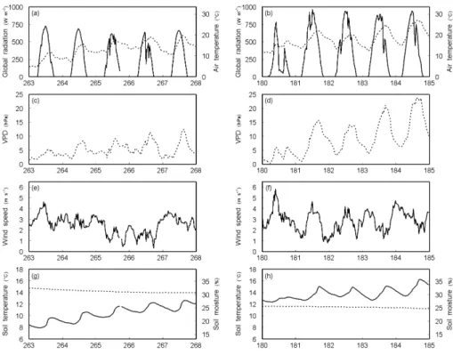
Within this sensitivity study, five days from each IOP that were chosen due to the good weather conditions and the good performance of the measuring devices were considered (IOP-1: 20–24 September 2007, day of year 263–267; IOP-2: 28 June– 2 July 2008, day of year 180–184). IOP-1 was carried out during a relatively wet and cool autumn, whereas during IOP-2 hot and dry summer weather prevailed, which
5
allows us to investigate different meteorological periods. The meteorological conditions during the two five-day periods are shown in Fig. 2. During IOP-1, global radiation, temperature and vapor pressure deficit were lower than during IOP-2. The wind speed reached comparable magnitudes during both IOPs. Soil conditions differed greatly during both IOPs, with a colder and wetter soil during IOP-1.
10
2.3 The ACASA model
The Advanced Canopy-Atmosphere-Soil Algorithm (ACASA, Pyles, 2000; Pyles et al., 2000), which was developed at the University of California, Davis, was used to model the turbulent fluxes of heat, water vapor and CO2 within and above the canopy. This multi-layer canopy-surface-layer model incorporates a diabatic, third-order closure
15
method to calculate turbulent transfer within and above the canopy on the theoretical basis of the work of Meyers and Paw U (1986, 1987). The multi-layer structure of ACASA is reflected in 20 atmospheric layers evenly distributed between the canopy and the air above extending to twice the canopy height, and in 15 soil layers. Leaf, stem and soil surface temperatures are calculated using the fourth-order polynomial
20
of Paw U and Gao (1988), allowing the calculation of temperatures of these compo-nents where these may deviate significantly from ambient air temperatures. Energy flux estimates consider multiple leaf-angle classes and direct as well as diffuse radia-tion absorpradia-tion, reflecradia-tion, transmission and emission. Plant physiological response to micro-environmental conditions is calculated by a combination of the Ball-Berry
stom-25
BGD
7, 4223–4271, 2010Sensitivity and uncertainty of
ACASA
K. Staudt et al.
Title Page
Abstract Introduction
Conclusions References
Tables Figures
◭ ◮
◭ ◮
Back Close
Full Screen / Esc
Printer-friendly Version Interactive Discussion
Discussion
P
a
per
|
Dis
cussion
P
a
per
|
Discussion
P
a
per
|
Discussio
n
P
a
per
|
from MAPS (Mesoscale Analysis and Prediction System; Smirnova et al., 1997, 2000). Additionally, canopy heat storage and canopy interception of precipitation are included in ACASA.
The model was adapted from a version from October 2009. The model source code was modified in two parts. The first change concerns the soil respiration calculations.
5
A soil moisture attenuation factor that is meant to reduce microbial soil respiration when soil moisture falls below the wilting point soil moisture was disabled in this study, as it not only reduced soil microbial respiration during dry periods but also enhanced respi-ration rates to unreasonably high values during wet periods, a finding that is consistent with Isaac et al. (2007). As in the original ACASA version, respirationRT at
tempera-10
tureTs is calculated with an Arrhenius type equation with basal respiration rateR0 at 0◦C and theQ10as input parameters (e.g., Hamilton et al., 2001):
RT=R0·exp(0.1·Ts·ln(Q10)) (1)
Here, R0 is given in (µmol m
−2
s−1), based on the surface area of the roots or mi-crobes. Soil respiration is simulated for microbes and roots separately, using Eq. (1),
15
and summed up to form the total soil respiration. Each of the two components is the sum of the respective respiration contributions from the 15 soil layers, weighted by the root fractions of these layers. To obtain the total soil respiration per ground surface area, it is assumed that the sum of the total root and microbe surface area resemble the leaf area index.
20
The second change in the source code was made within the plant physiology sub models in the calculation of photosynthesis. The temperature dependence of the max-imum catalytic activity of Rubisco at saturated ribulose biphosphate (RuBP) and satu-rated CO2,Vcmax(µmol m−
2
s−1) follows a third-order polynomial given by Kirschbaum and Farquhar (1984), which was derived from measurements made in a temperature
25
BGD
7, 4223–4271, 2010Sensitivity and uncertainty of
ACASA
K. Staudt et al.
Title Page
Abstract Introduction
Conclusions References
Tables Figures
◭ ◮
◭ ◮
Back Close
Full Screen / Esc
Printer-friendly Version Interactive Discussion
Discussion
P
a
per
|
Dis
cussion
P
a
per
|
Discussion
P
a
per
|
Discussio
n
P
a
per
|
replaced by the temperature dependence ofVcmax as used in the C3leaf sub-module PSN6 of the model SVAT-CN (Falge et al., 1996, 2005):
Vcmax=Vcmax25
exp[∆Ha·(TK−Tref)/(R·TK·Tref)]·(1+exp[(∆S·Tref−∆Hd)/(R·Tref)])
1+exp[(∆S·TK−∆Hd)/(R·TK)]
(2)
whereTK is the leaf temperature (in K),Ris the gas constant (8.31 J mol−1K−1),Vcmax25 is the maximum carboxylation rate at a reference temperatureTref of 298.15 K, ∆S is
5
an entropy term (655 J mol−1K−1), and ∆Ha and ∆Hd are the activation energy and energy of deactivation (both in J mol−1,∆Hdset to 200 000 J mol
−1
), respectively. The output of the ACASA model comprises profiles of mean quantities, flux profiles including the components of the CO2 exchange, profiles of the third order moments and profiles of the soil properties. For the purpose of the sensitivity analysis, only the
10
turbulent and radiative fluxes above the canopy were considered. The performance of other quantities at our site, such as the flux profiles, was assessed in a different study (Staudt et al., 2010).
2.4 The GLUE methodology
To evaluate the sensitivity and uncertainty of the ACASA model, the Generalized
Likeli-15
hood Uncertainty Estimation (GLUE) method, which has been proposed by Beven and Binley (1992) and is described in detail in Beven et al. (2000), was employed here. The basic idea of the GLUE methodology is the principle of equifinality, which here means that one does not expect a single optimum parameter set for a model but rather many sets of parameters that give equally good model results. In a Monte Carlo simulation
20
framework, a large number of random sets of parameters are derived from uniform distributions across specified parameter ranges. The model results are then evaluated through the calculation of likelihood measures (see below). Based on the values of these likelihood measures and a predefined threshold value to distinguish between ac-ceptable and not acac-ceptable runs, “behavioral” parameter sets can be identified and
BGD
7, 4223–4271, 2010Sensitivity and uncertainty of
ACASA
K. Staudt et al.
Title Page
Abstract Introduction
Conclusions References
Tables Figures
◭ ◮
◭ ◮
Back Close
Full Screen / Esc
Printer-friendly Version Interactive Discussion
Discussion
P
a
per
|
Dis
cussion
P
a
per
|
Discussion
P
a
per
|
Discussio
n
P
a
per
|
“non-behavioral” parameter sets rejected from further analysis. In a next step, uncer-tainty bounds for each time step are deduced from the cumulative distribution of the output variables ranked by the likelihood measure.
A number of subjective decisions have to be made within the GLUE methodology. These are the definition of the parameter ranges and the prior parameter distributions
5
as well as the choice of the likelihood measure applied and the corresponding value of the threshold of acceptability. However, these decisions have to be made explicitly and are therefore open to debate.
The data preparation and the analysis following the GLUE methodology was done with the statistical and graphics software package R (R Development Core Team,
10
2008).
2.4.1 Parameters and parameter ranges
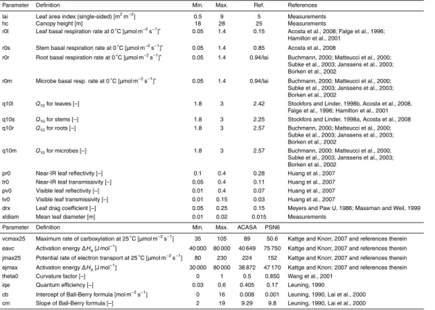
The original version of the ACASA model requires a number of “external”, user defined geographical, morphological and physiological parameters (see upper part of Table 2). In this study constant values were used over the whole profile to keep the number of
15
investigated parameters limited. The overall number of the external parameters used within this study is 16, and a few external parameters were held constant, such as the soil type and the measured normalized LAI profile (Fig. 1b, fitted following Simon et al., 2005).
Additionally, 8 parameters from the photosynthesis and stomatal conductance
sub-20
models were included in this sensitivity analysis (see lower part of Table 2, in the fol-lowing called “internal” parameters). In the original version of the ACASA model, only Vcmax25and a so-called “water use efficiency factor” can be defined by the user.Jmax25 is then defined as 2.41·Vcmax25. The “water use efficiency factor” wue alters the leaf stomatal conductance to water vapor gs,w (Su et al., 1996) calculated with the
Ball-25
Berry formula.
gs,w=
cm·An
cs ·rhs+cb
· 1
BGD
7, 4223–4271, 2010Sensitivity and uncertainty of
ACASA
K. Staudt et al.
Title Page
Abstract Introduction
Conclusions References
Tables Figures
◭ ◮
◭ ◮
Back Close
Full Screen / Esc
Printer-friendly Version Interactive Discussion
Discussion
P
a
per
|
Dis
cussion
P
a
per
|
Discussion
P
a
per
|
Discussio
n
P
a
per
|
with An the net CO2 uptake rate at the leaf surface, cs the CO2 concentration, rhs
the relative humidity at the leaf surface and cb the intercept and cm the slope of the Ball-Berry formula. For the remaining plant physiological parameters, values from the literature were adapted (Su et al., 1996). However, we chose to independently vary all listed photosynthesis and stomatal conductance parameters in this sensitivity study,
5
thus wue was set to 1 and the ratio ofVcmax25andJmax25was not fixed.
The parameter ranges for this sensitivity analysis include the original parameter val-ues used in ACASA and PSN6, which are listed as reference valval-ues in Table 2. Fur-thermore, values from the literature for spruce or coniferous forests in general were collected to cover a realistic range of values. Where possible, parameter ranges were
10
determined from direct measurements.
As there was no evidence for other statistical distributions, all parameter ranges were assigned a uniform distribution. Random sets of parameters were produced for a large number of model runs (20 000). Parameters were independently randomized, with the exception of the parameters for microbial and root respiration which were set
15
to the same values, meaning that root and microbial respiration each contribute 50% to total soil respiration (mean of values for temperate coniferous forests, as listed in Subke et al., 2006). Even though RuBP carboxylation and regeneration are linked to each other, the parametersJmax25andVcmax25were varied independently. The chosen parameter ranges allowed a ratio ofJmax25andVcmax25between 0.8 and 6.5, but values
20
between one and three as found to be typical by Kattge and Knorr (2007) were most frequent.
The model was run for the two chosen time periods for all randomly generated pa-rameter sets and the resulting radiative and turbulent fluxes and the net ecosystem exchange (NEE) above the canopy stored for further evaluation.
25
2.4.2 Likelihood measures
BGD
7, 4223–4271, 2010Sensitivity and uncertainty of
ACASA
K. Staudt et al.
Title Page
Abstract Introduction
Conclusions References
Tables Figures
◭ ◮
◭ ◮
Back Close
Full Screen / Esc
Printer-friendly Version Interactive Discussion
Discussion
P
a
per
|
Dis
cussion
P
a
per
|
Discussion
P
a
per
|
Discussio
n
P
a
per
|
and has been used in previous studies (Beven et al., 2000). For each of the radiative and turbulent fluxes and the NEE above the canopy, likelihood measures were calcu-lated for 20000 runs from the observed and the simucalcu-lated data:
L(θj|Y)=
E
C (4)
Here, L(θj|Y) is the likelihood measure for the jth model run with parameter set θj
5
conditioned on the observations Y. The normalizing constantC was set to 1 in our study.E is the coefficient of efficiency (Nash and Sutcliffe, 1970)
E=1−
P
(Oj−Pj)
2
P
(Oj−O)2
(5)
whereOis observed andP model simulated data. The coefficient of efficiencyE varies from minus infinity to 1, and values close to 1 indicate a good agreement of modeled
10
and measured data. This goodness of fit measure has the advantage that the value of zero serves as a convenient reference point, indicating that model runs that result in coefficients of efficiency of zero are as good as the observed mean and those that correspond to negative values perform worse than the observed mean (Legates and McCabe, 1999). The coefficient of efficiency is a widely used likelihood measure within
15
GLUE studies (e.g., Freer et al., 1996; Schulz et al., 1999, 2001; Liebethal et al., 2005; Franks et al., 1997; Choi and Beven, 2007; Poyatos et al., 2007).
The second subjective element mentioned above is the definition of the behavioral threshold. Likelihood measures that are lower than the behavioral threshold are given a value of 0, which means that these parameter sets are excluded from further analysis.
20
A different approach was followed by Prihodko et al. (2008) and Lamb et al. (1998) who used the top 10% runs for further analysis instead of defining a threshold value. We also chose the top 10% runs, which has the advantage that the number of behavioral runs for all variables considered is the same, despite considerably deviating ranges of the likelihood measures achieved by the different fluxes.
BGD
7, 4223–4271, 2010Sensitivity and uncertainty of
ACASA
K. Staudt et al.
Title Page
Abstract Introduction
Conclusions References
Tables Figures
◭ ◮
◭ ◮
Back Close
Full Screen / Esc
Printer-friendly Version Interactive Discussion
Discussion
P
a
per
|
Dis
cussion
P
a
per
|
Discussion
P
a
per
|
Discussio
n
P
a
per
|
To combine two or more likelihood measures, various combination equations are possible (Beven and Freer, 2001). Here, combined likelihoods are achieved by applying Bayes equation in the following form:
L(θj|Y)=
L1(θj|Y)·L2(θj|Y)·L3(θj|Y)
C (6)
which means that the normalized likelihood measures L1, L2 and L3 are treated as
5
a priori distributions and are rescaled. The normalizing constantCwas again set to 1. We applied this equation to the best 10% model runs of the sensible and latent heat fluxes and the NEE for the two IOPs separately.
While other GLUE studies on SVAT-models (e.g., Prihodko et al., 2008; Mo and Beven, 2004) concentrate on a combined likelihood measure to achieve the best overall
10
performance for all fluxes which is a precondition for land surface schemes, this study also focuses on the performance of individual fluxes as we are highly interested in short term fluctuations of these fluxes.
2.4.3 Parameter sensitivity
The GLUE methodology focuses on the model response to parameter sets rather than
15
to single parameter values. Nevertheless, the sensitivity of single parameters can be evaluated with the help of sensitivity graphs, which are scatter plots of likelihood measures versus parameter values for the behavioral parameter sets. Thus, the mul-tidimensional parameter response surface is projected onto a single parameter axis (Fig. 3a–f for the sensible heat flux (H), the latent heat flux (LE) and the NEE against
20
leaf area index, lai, during IOP-1 and IOP-2).
In a next step, cumulative frequencies of the parameters for the final behavioral model runs were compared to the original uniform distribution (Franks et al., 1999; Schulz et al., 1999, Fig. 3g and h for leaf area index lai during IOP-1 and IOP-2). Here, the three single-objective as well as the combined likelihood measures were
an-25
BGD
7, 4223–4271, 2010Sensitivity and uncertainty of
ACASA
K. Staudt et al.
Title Page
Abstract Introduction
Conclusions References
Tables Figures
◭ ◮
◭ ◮
Back Close
Full Screen / Esc
Printer-friendly Version Interactive Discussion
Discussion
P
a
per
|
Dis
cussion
P
a
per
|
Discussion
P
a
per
|
Discussio
n
P
a
per
|
to right-up corner of the cumulative distribution plots. If there is no difference in the original distribution and the distribution of the behavioral simulations, the parameter is considered as insensitive, whereas a deviation from the diagonal line indicates param-eter sensitivity. The shape of the cumulative frequency curves gives an idea of optimal parameter values, as the area of steepest slope points out where the majority
param-5
eter values are found (Prihodko et al., 2008). With a Kolmogorov-Smirnov (K-S) test the equality of the cumulative frequency of the behavioral model runs and the original uniform distributions can be tested and the significance of any differences determined. The parameters to which the model is sensitive were identified if the K-S test statistic was significant at thep=0.01 level. The K-S value was used to rank the parameters
10
according to their significance, with higher K-S values indicating a higher sensitivity. This approach was followed by Prihodko et al. (2008) in analyzing a SVAT-model and was also successfully used in previous sensitivity tests for other model classes (e.g., Meixner et al., 1999; Spear and Hornberger, 1980).
2.4.4 Uncertainty estimation
15
Uncertainty bounds were calculated for each flux at each time step t for the single-objective and the combined measures with (Beven and Freer, 2001):
P( ˆZt< z)= B
X
i=1
LhM(θi)|Zˆt,i< z
i
(7)
where ˆZt,i is the value of variableZ at timetsimulated by modelM(θi) with parameter setθi. Output variables from the behavioral runs for each time step were ranked and its
20
BGD
7, 4223–4271, 2010Sensitivity and uncertainty of
ACASA
K. Staudt et al.
Title Page
Abstract Introduction
Conclusions References
Tables Figures
◭ ◮
◭ ◮
Back Close
Full Screen / Esc
Printer-friendly Version Interactive Discussion
Discussion
P
a
per
|
Dis
cussion
P
a
per
|
Discussion
P
a
per
|
Discussio
n
P
a
per
|
et al. (2008). Beven and Freer (2001) note that these quantiles are conditional on the model input data, the parameter sets, the observations and the choice of likelihood measure.
3 Results
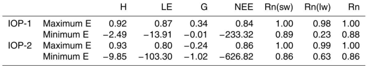
3.1 Ranges of likelihood measure
5
The maximum values as well as the ranges of the coefficient of efficiency E (Table 3) were very different for the seven fluxes considered here. Only for net radiation (Rn) and the short-wave radiation budget (Rn(sw)) were values of 1 reached for both IOPs, which shows, in combination with a small variability of the likelihood measures, a very good agreement of observed and modeled data. The maximum values for the sensible
10
heat flux (H) were close to the values for net radiation, whereas the range was larger. For the latent heat flux (LE) and NEE, the variability was much wider. The ranges of the coefficient of efficiency for the sensible heat flux, the latent heat flux and the NEE were considerably larger for IOP-2 than for IOP-1. Maximum values for the sensible heat flux and the NEE were similar for both IOPs, whereas there were differences between
15
the IOPs for the latent heat flux with larger values during IOP-1. For the radiation budgets, only the long-wave radiation budget had a larger range and a slightly lower maximum value during IOP-1 than during IOP-2. Maximum coefficients of efficiency for the ground heat flux (G) reached only very low values.
For further analysis, we retained the top 10% runs and concentrated on the sensible
20
and latent heat fluxes and the NEE. For all fluxes except the NEE during IOP-2, the coefficients of efficiency of the best 10% runs were in the range between one and zero (Fig. 3). Negative coefficients of efficiency indicate that the simulation is worse than the observed mean, thus such model runs are unwanted. These model runs were also excluded from further analysis, resulting in only 1901 model runs (9.5%) for the NEE
25
BGD
7, 4223–4271, 2010Sensitivity and uncertainty of
ACASA
K. Staudt et al.
Title Page
Abstract Introduction
Conclusions References
Tables Figures
◭ ◮
◭ ◮
Back Close
Full Screen / Esc
Printer-friendly Version Interactive Discussion
Discussion
P
a
per
|
Dis
cussion
P
a
per
|
Discussion
P
a
per
|
Discussio
n
P
a
per
|
For all tested runs, the modeled radiative flux budgets, with exception of the long wave radiation budget during IOP-1, were in very good agreement with the measured values. Therefore, the effort to better parametrize the model will be directed to the other fluxes. The ground heat flux proved to achieve only small likelihood measure values, especially during IOP-2. This is mainly attributable to the ground heat flux
measure-5
ments, which are single-point measurements and were, in our case, influenced by sunspots in the late afternoon resulting in very high ground heat fluxes lasting for only a short period. As the model represents an area rather than a point, any direct compar-ison of these data has to be done carefully, and thus the ground heat flux was excluded from further analysis. For sensible and latent heat flux as well as the NEE, the footprint
10
of the measurements (Siebicke, 2008) is well within the range of the horizontal spatial scale of the ACASA model, which represents a flux footprint of about 104to 106m2.
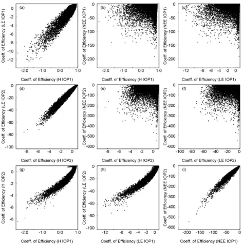
The performance of the parameter sets for the three fluxes are compared in Fig. 4 (4a–c for IOP-1, 4d–f for IOP-2). There was a correlation of the coefficients of efficiency for the sensible and the latent heat flux with a similar relative model performance for
15
all parameter sets, but there is no correlation for the sensible and latent heat fluxes with the NEE. The number of parameter sets that are within the 10% best parameter sets for all three fluxes is very much reduced from the 2000 (1901 for NEE in IOP-2) parameter sets to 94 for IOP-1 and 87 for IOP-2. The last three panels of Fig. 4 compare each of the coefficients of efficiency for the three fluxes for IOP-1 with those
20
for IOP-2. For the NEE, there is a good correlation between the two IOPs, whereas for the other two fluxes the scatter plots are somewhat bow-shaped. Combining the coefficients of efficiency for all three fluxes for the two IOPs yielded only 7 behavioral parameter sets.
3.2 Sensitivity graphs
25
BGD
7, 4223–4271, 2010Sensitivity and uncertainty of
ACASA
K. Staudt et al.
Title Page
Abstract Introduction
Conclusions References
Tables Figures
◭ ◮
◭ ◮
Back Close
Full Screen / Esc
Printer-friendly Version Interactive Discussion
Discussion
P
a
per
|
Dis
cussion
P
a
per
|
Discussion
P
a
per
|
Discussio
n
P
a
per
|
for the latent heat flux, there was a large difference of ranges of coefficients of effi -ciency for the 10% best model runs for the two IOPs with values for IOP-1 that were all larger than the maximum values for IOP-2. All fluxes show a high degree of sensitivity to the lai for both IOPs, with a higher frequency of lai values within the lower half of the lai range for all fluxes. Only for the latent heat flux for IOP-1 does the distribution peak
5
at a higher value of approximately 4 m2m−2 and does not cover values smaller than 2 m2m−2.
To directly compare the sensitivity of the parameters for the different fluxes, the cu-mulative frequency of each of the parameters for the 10% best runs were plotted and compared to a uniform parameter distribution, indicated by the diagonal line (Fig. 3g
10
and h). Slopes of the cumulative frequency curves that deviate from the slope of the di-agonal line indicate parameter sensitivity and more or less frequent parameter ranges for larger or smaller slopes, respectively. For the lai, the features as explained above can easily be seen in the plots of cumulative frequency. For all fluxes the steepest slopes in the curves (i.e. the largest derivative) and therefore the optimal parameter
15
values are in a range of lai values of 0.5 to 5 m2m−2, which is lower than the reference value for the Waldstein-Weidenbrunnen site of 5 m2m−2. For the sensible heat flux for IOP-1 and the latent heat flux for both IOPs, lai values lower than a certain thresh-old were not found in the behavioural parameter sets, indicated by no increase in the cumulative frequency curves across the lower parameter range. Similarly, lai values
20
larger than a certain threshold value did not appear within the behavioural parameter sets for the sensible heat flux for both IOPs and for the latent heat flux for IOP-2. The cumulative frequency curves for the combined coefficients of efficiency for both IOPs have a more pronounced shape than the other curves, indicating optimal lai values of approximately 2 m2m−2and no lai values below and above a lower and upper lai value,
25
respectively.
BGD
7, 4223–4271, 2010Sensitivity and uncertainty of
ACASA
K. Staudt et al.
Title Page
Abstract Introduction
Conclusions References
Tables Figures
◭ ◮
◭ ◮
Back Close
Full Screen / Esc
Printer-friendly Version Interactive Discussion
Discussion
P
a
per
|
Dis
cussion
P
a
per
|
Discussion
P
a
per
|
Discussio
n
P
a
per
|
deviates much from the diagonal line representing the uniform distribution. As stem respiration contributes little to total respiration, it is not surprising that parameters for stem respiration are not among the influential model parameters. The cumulative fre-quency curves of the other two parameters displayed in Fig. 5, the quantum efficiency, iqe (c and d), and the basal respiration rate for soil microbes, r0m (e and f), deviate
5
from the diagonal for one or all fluxes. The parameter iqe, a parameter utilized in the plant physiology sub-modules, appears as an influential parameter for all three fluxes. For the sensible and latent heat fluxes, the cumulative frequency curve has a similar shape with a larger slope for lower values and a smaller slope for high iqe values. The shape for the NEE curve is the opposite, with smaller gradients for low iqe values.
10
The NEE is strongly sensitive to the value of the microbe basal respiration rate r0m with a steeper slope of the curve at lower basal respiration rates and a lesser slope for values in the upper range of the basal respiration rates, indicating optimal param-eter values within the lower third of the paramparam-eter range. For r0m and iqe for IOP-1, the curve for the combined likelihood measure follows the NEE curve closely, whereas
15
the combined likelihood measure is not sensitive to iqe for IOP-2, probably due to the opposing cumulative frequency curves for the NEE and the other two fluxes.
Whereas all parameters in Fig. 5 showed a similar behavior in both IOPs, the three parameters displayed in Fig. 6 experience a different response for the two IOPs. For the near-IR leaf reflectivity, pr0, the curves for latent heat flux and the NEE in Fig. 6a
20
and b do not deviate from the diagonal line, thus these fluxes show no sensitivity to the value of pr0. Only the curve for the sensible heat flux for 1, but not for IOP-2, indicate a higher frequency of higher pr0 values. Lower values of the intercept of the Ball-Berry formula, cb, are more frequent within behavioral parameter sets for the sensible and latent heat fluxes for IOP-2 (Fig. 6c and d). Values for cb in behavioral
25
BGD
7, 4223–4271, 2010Sensitivity and uncertainty of
ACASA
K. Staudt et al.
Title Page
Abstract Introduction
Conclusions References
Tables Figures
◭ ◮
◭ ◮
Back Close
Full Screen / Esc
Printer-friendly Version Interactive Discussion
Discussion
P
a
per
|
Dis
cussion
P
a
per
|
Discussion
P
a
per
|
Discussio
n
P
a
per
|
heat fluxes. Whereas for the NEE for both IOPs the behavioral parameter sets contain more values from the upper half of the parameter range, the cumulative frequency curves for the other two fluxes suggest optimal parameter values from the lower half of the parameter ranges, with a much stronger response for IOP-2, where values are completely confined to the lower half of the parameter range.
5
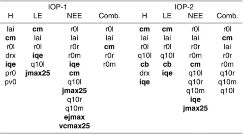
To quantify whether the distribution of parameter values for the 10% best model runs follows the uniform distribution or not, and thus to identify the parameters the model is sensitive to and to list these parameters in order of importance, the Kolmogorov-Smirnov test was performed. Table 4 gives an overview of the sensitive model param-eters for the respective fluxes according to the Kolmogorov-Smirnov test for IOP-1 and
10
IOP-2.
There was a difference in the number of sensitive parameters between the two IOPs with a larger number of sensitive parameters for NEE for IOP-1 than for IOP-2 and a larger number of sensitive parameters for the combined fluxes for IOP-2 than for IOP-1.
15
As the lai appears as the first or one of the first parameters in the parameter rankings for all fluxes, the importance of this parameter as one of the most influential parameters is illustrated once more. The other two plant morphological parameters, the canopy height, hc, and the mean leaf diameter, xldiam, are not listed among the influential parameters. The leaf drag coefficient, drx, used in the third order closure turbulence
20
subroutines only appears in the parameter rankings for the sensible heat flux.
Also among the most influential parameters for all fluxes are the parameters de-termining leaf respiration, with the leaf basal respiration rate, r0l, and the Q10 of leaf respiration, q10l. The parameters for stem respiration (r0s, q10s) do not appear in the parameter rankings, whereas the parameters for root and microbial respiration (r0r,
25
BGD
7, 4223–4271, 2010Sensitivity and uncertainty of
ACASA
K. Staudt et al.
Title Page
Abstract Introduction
Conclusions References
Tables Figures
◭ ◮
◭ ◮
Back Close
Full Screen / Esc
Printer-friendly Version Interactive Discussion
Discussion
P
a
per
|
Dis
cussion
P
a
per
|
Discussion
P
a
per
|
Discussio
n
P
a
per
|
The parameters of the photosynthesis and stomatal conductance subroutines con-tribute to the ranked parameters in roughly the same proportion as they do to the over-all number of investigated parameters for the sensible heat flux and the NEE, but in a larger proportion for the latent heat flux and in a smaller proportion for the combined fluxes. Of the parameters that determine the temperature dependence of the maximum
5
catalytic activity of RubiscoVcmax, only the maximum rate of carboxylation, vcmax25, appears to be influential for the NEE for IOP-1. The corresponding activation energy, eavc, does not appear in the parameter rankings. The picture for the maximum rate of whole-chain electron transport at saturated lightJmaxis different, with the potential rate of electron transport at 25◦C, jmax25, appearing as an influential parameter for the
10
NEE for both IOPs and the latent heat flux for IOP-1, and the activation energy, ejmax, appearing also for NEE for IOP-1.
The radiation dependence of the potential rate of whole-chain electron transport is affected by the curvature factor, theta0, and the quantum efficiency, iqe, with the latter being influential for all fluxes except the combined fluxes, and the former not being
15
influential for any flux. The slope of the Ball-Berry formula, cm, to calculate stomatal conductance appears for all fluxes and the combined fluxes as the first or one of the first parameters, thus as one of the most influential parameters. In contrast, the second parameter in the Ball-Berry formula, its intercept cb, only appears for the sensible and latent heat fluxes in IOP-2 in combination with cm.
20
3.3 Model uncertainty
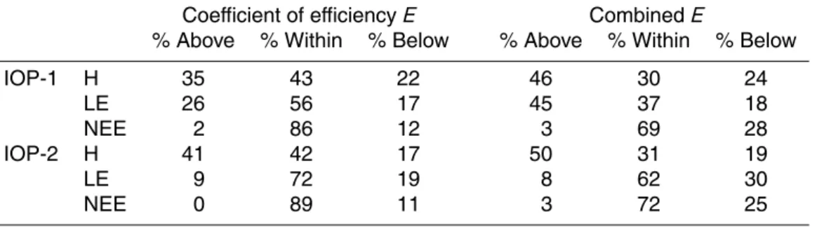
Predictive uncertainty bounds were calculated for each flux for the individual best 10% model runs and the model runs resulting from the combination of all three likelihood measures for both IOPs (Figs. 7 and 8). Table 5 lists the percentage of observations that are enclosed by the uncertainty bounds and those that lie without. In general, the
25
BGD
7, 4223–4271, 2010Sensitivity and uncertainty of
ACASA
K. Staudt et al.
Title Page
Abstract Introduction
Conclusions References
Tables Figures
◭ ◮
◭ ◮
Back Close
Full Screen / Esc
Printer-friendly Version Interactive Discussion
Discussion
P
a
per
|
Dis
cussion
P
a
per
|
Discussion
P
a
per
|
Discussio
n
P
a
per
|
quite well. But the model seems to respond to environmental conditions faster than the observations, with an earlier onset of growing sensible heat fluxes in the morning and of decreasing fluxes in the afternoon, resulting in a slight time shift. Therefore, the percentage of observations within the uncertainty bounds for the sensible heat flux is below 50% (Table 5). The model was not able to capture maximum daytime latent
5
heat flux values for some days during both IOPs. During night time, latent heat fluxes for IOP-1 were also frequently underestimated by the model. For latent heat fluxes the percentage of observations within the uncertainty bounds is larger for IOP-2 than for IOP-1, whereas for the other two fluxes it is very similar for both IOPs (Table 5). Un-certainty bounds for the NEE are the largest of all fluxes, but also enclose the highest
10
percentage of observations during both IOPs.
For all fluxes, there was a smaller percentage comprised of uncertainty bounds con-strained on all three fluxes than those concon-strained on individual fluxes. This is espe-cially evident for the NEE for IOP-2, where maximum daytime values are no longer covered by the combined uncertainty bounds (Fig. 8).
15
4 Discussion
First of all, it should be noted that the outcome of this sensitivity study only applies for the Waldstein-Weidenbrunnen site and furthermore is only valid for these two time periods, as results of an analysis following the GLUE methodology are always condi-tional not only on the parameter sets and the choice of likelihood measure but also
20
on the model input data and the observations (Beven and Freer, 2001). Additionally, it has to be kept in mind that the eddy-covariance measurements, which served as com-parison values to the modeled fluxes, might be afflicted with errors. The uncertainties of eddy-covariance measurements are a recent field of research (e.g., Hollinger and Richardson, 2005; Mauder et al., 2006; Foken, 2008). Following Mauder et al. (2006),
25
BGD
7, 4223–4271, 2010Sensitivity and uncertainty of
ACASA
K. Staudt et al.
Title Page
Abstract Introduction
Conclusions References
Tables Figures
◭ ◮
◭ ◮
Back Close
Full Screen / Esc
Printer-friendly Version Interactive Discussion
Discussion
P
a
per
|
Dis
cussion
P
a
per
|
Discussion
P
a
per
|
Discussio
n
P
a
per
|
sensible heat flux and 20% or 40 W m−2for the latent heat flux. Mitchell et al. (2009) considered the uncertainty in annual NEE estimates in the selection of behavioral pa-rameter in a GLUE study. However, measurement uncertainties were not included in our GLUE analysis.
4.1 Parameter sensitivity
5
About one third to one half of the input parameters were identified as influential pa-rameters, including internal as well as external parameters. However, the so-called problem of parameter equifinality was detected in ACASA. For many parameters, very good as well as very poor results for the sensible and latent heat flux and the NEE were obtained for every parameter value in the examined parameter range. This was
10
also reported in several studies examining the sensitivity of parameters in complex process-based models (e.g., Franks et al., 1997; Schulz et al., 2001; Prihodko et al., 2008).
The two periods of different meteorological conditions, a cold and wet autumn in 2007 and a hot and dry summer in 2008, allowed the study of seasonal variations in
15
parameter sensitivity. The sensitivity of the fluxes to a range of parameters, such as the basal soil respiration rates (see parameters in Fig. 5), was similar for both periods, whereas a few parameters experienced a different response to the parameter values for the two time periods (e.g. pr0 Fig. 6). This was especially evident for the slope of the Ball-Berry formula, cm, with a stronger sensitivity of the latent and sensible heat fluxes
20
to this parameter for IOP-2 (Fig. 6). For this drier and warmer period, the best model re-sults were achieved with a lower cm value than for the colder and wetter IOP1. This is in line with the suggestions of Tenhunen et al. (1990) and Baldocchi (1997) to reduce the slope of the Ball-Berry formula with decreasing water availability for the simulation of H2O and CO2exchange of a Mediterranean and a temperature broad-leaved forest,
re-25
BGD
7, 4223–4271, 2010Sensitivity and uncertainty of
ACASA
K. Staudt et al.
Title Page
Abstract Introduction
Conclusions References
Tables Figures
◭ ◮
◭ ◮
Back Close
Full Screen / Esc
Printer-friendly Version Interactive Discussion
Discussion
P
a
per
|
Dis
cussion
P
a
per
|
Discussion
P
a
per
|
Discussio
n
P
a
per
|
number and ranking of influential parameters (Table 4) consequently varies for the two time periods, indicating the need to seasonally adjust several parameter values. But as only two short periods are considered here, such recommendations are of limited justifiability. In order to draw general conclusions about the seasonality of parameters and to cover all relevant processes, it is necessary to include much longer time
peri-5
ods with a larger meteorological variability, as was done by Prihodko et al. (2008). An extension of the time period studied was also suggested as a possible solution to the parameter equifinality problem by Schulz et al. (2001).
Our findings of parameters that appeared to be influential in our sensitivity analy-sis revealed similarities with results from other sensitivity studies or studies that used
10
inversion methods for parameter estimation. Even though other models – including different process descriptions and thus different parameters investigated – were anal-ysed, stomatal parameters were also among the most sensitive or best constrained parameters (Mitchell et al., 2009; Prihodko et al., 2008; Knorr and Kattge, 2005). Wang et al. (2001) included the slope of the Ball-Berry formula in their parameter estimation,
15
whereas all fluxes proved to be insensitive to the intercept of the Ball-Berry formula. Our observations revealed a similar result, with the slope of the Ball-Berry formula being among the most influential parameters and its intercept being not influential for any flux. Furthermore, the parameter inversion performed by Knorr and Kattge (2005) found that amongst the photosynthesis parameters most information was gained for
20
quantum efficiency and maximum carboxylation rate. We found quantum efficiency to be an influential parameter; however, maximum carboxylation rate was less influen-tial. As in our study, strong sensitivity to the leaf area index was found by Mitchell et al. (2009).
The sensitivity to parameter values for the three studied fluxes was not the same
25
BGD
7, 4223–4271, 2010Sensitivity and uncertainty of
ACASA
K. Staudt et al.
Title Page
Abstract Introduction
Conclusions References
Tables Figures
◭ ◮
◭ ◮
Back Close
Full Screen / Esc
Printer-friendly Version Interactive Discussion
Discussion
P
a
per
|
Dis
cussion
P
a
per
|
Discussion
P
a
per
|
Discussio
n
P
a
per
|
with cumulative frequency plots indicating optimal parameter values from the lower part of the parameter range for one flux and from the upper part of the parameter range for the other flux (e.g. iqe in Fig. 5). Thus, difficulties arise when trying to deduce optimal parameter values from the results of this study, and the model user has to decide in favor of either the latent heat flux or the NEE. The sensible heat flux either showed
5
a response similar to that of the latent heat flux or was not sensitive to the respective parameter.
A complex process-based model like ACASA requires a large number of input pa-rameters. In this study, 24 parameters were of interest and concurrently varied to create 20 000 random parameter sets, which is very few with regard to the number of
param-10
eters. A much larger number of parameter sets would be required to sample the whole range of variation in combinations of parameters, which would hardly be realizable due to the large computational power required. However, as with Prihodko et al. (2008), who had an even larger number of parameters, we expect that an important range of the parameter space is already covered by 20 000 model runs.
15
In order to not only cover a larger range of variation in combinations of parame-ters but also to reduce the problem of parameter equifinality, the results of the present GLUE analysis could be used to fix relatively insensitive parameter values, to constrain parameter ranges and to improve the model structure for a subsequent GLUE analysis (Prihodko et al., 2008). Alternatively, Schulz et al. (2001) not only suggest prescribing
20
as many parameter values as possible using measurements to reduce the degrees of freedom, but also mention the gap between scales of measured parameters and pa-rameters needed to run models. For the photosynthesis papa-rameters, this is especially evident, where parameters of the gas exchange response of a few sample leaves is used as average leaf parameterization of the entire stand.
25
4.2 Identification of structural weaknesses of the model
BGD
7, 4223–4271, 2010Sensitivity and uncertainty of
ACASA
K. Staudt et al.
Title Page
Abstract Introduction
Conclusions References
Tables Figures
◭ ◮
◭ ◮
Back Close
Full Screen / Esc
Printer-friendly Version Interactive Discussion
Discussion
P
a
per
|
Dis
cussion
P
a
per
|
Discussion
P
a
per
|
Discussio
n
P
a
per
|
choice of likelihood measure (Beven and Freer, 2001). Therefore, it is difficult to deter-mine whether the observed errors are the result of structural weaknesses of the model or errors in the input data or the observations. Nevertheless, Mitchell et al. (2009) demonstrated how to use a GLUE study to detect problems in model structure. Our analysis also revealed indications to structural weaknesses, such as in the soil
respi-5
ration calculations of the model, which will be discussed in the following.
For the NEE, the basal respiration rates for the soil and the leaves as well as the lai are the most influential parameters for both IOPs. On the one hand, this could suggest respiration as the most important process for the CO2 exchange within the ACASA model, but on the other hand could also be caused by an inappropriate choice of
pa-10
rameter ranges, as the results are conditional on all the subjective choices concerning likelihood measures, rejection criteria and parameter ranges. The equations governing the soil respiration calculations were introduced in Chap. 2.3, with the basal soil res-piration rates r0r and r0m being defined per root area and per microbial surface area, respectively. The sum of the root and microbial surface areas are, in turn, assumed to
15
be equal to the lai value. Thus, the effective basal respiration rate for the soil strongly depends on the lai, and an interaction of these two parameters is expected. The scatter plot of the parameters basal respiration rate of the roots, r0r, versus the leaf area index, lai, for coefficients of efficiency for the NEE larger than 0.6 confirms this assumption (Fig. 9). The effective basal respiration rate for the roots (r0r· lai) for most model runs
20
was between 0.2 and 2 µmol m−2s−1, which encompasses values measured for spruce sites (0.65 to 1.16 µmol m−2s−1, references see Table 2). Figure 9 also illustrates that the parameter ranges as chosen result in a very large possible range for the effective basal respiration rate, which leads to very large and inappropriate root respiration for combinations of large r0r and large lai, dominating the NEE and leading to low model
25
performances.
BGD
7, 4223–4271, 2010Sensitivity and uncertainty of
ACASA
K. Staudt et al.
Title Page
Abstract Introduction
Conclusions References
Tables Figures
◭ ◮
◭ ◮
Back Close
Full Screen / Esc
Printer-friendly Version Interactive Discussion
Discussion
P
a
per
|
Dis
cussion
P
a
per
|
Discussion
P
a
per
|
Discussio
n
P
a
per
|
there were variations of this ratio observed, for example variations with age for young eucalyptus trees (O’Grady et al., 2006) and with elevation within a tropical mountain forest in Ecuador (R ¨oderstein, 2006). We therefore suggest using the basal root res-piration rate based on the soil surface as it is measured at many sites, rather than assuming a root respiration rate based on root surface and assuming the root surface
5
as being equal to the lai. Such a reduction of complexity, even though it only con-cerns one sub model, could help to reduce the problem of parameter equifinality, as suggested by Schulz et al. (2001) and Franks et al. (1997).
4.3 Predictive uncertainty of the modeled fluxes
The ACASA model was capable of reproducing all fluxes reasonably well as reflected
10
by the uncertainty bounds in Figs. 7 and 8. For the latent heat flux, maximum daily values were not captured by the model for IOP-1. For the first days, this underestima-tion can probably be attributed to evaporaunderestima-tion from intercepunderestima-tion due to a rainy period before day 263, which was not included in the simulation period and therefore cannot be adequately represented by the model. During each of the IOPs there was one night
15
where measured fluxes behaved differently than during all other nights, with all fluxes being close to zero (night 265/266 for IOP-1 and night 181/182 for IOP-2). This diver-gent behavior was not simulated by ACASA. Instead, the modeled fluxes during these nights were comparable in magnitude to the fluxes of the other nights. During these two nights measured wind speeds were much lower (Fig. 2), stabilities higher and friction
20
velocities smaller than during the other nights, indicating decoupling of the canopy and the air above. Close to the soil surface, decoupling was also observed during these periods (Riederer, 2009). The ACASA model is probably not capable of representing this process and therefore overestimates the fluxes above the canopy during periods of strong decoupling.
25
BGD
7, 4223–4271, 2010Sensitivity and uncertainty of
ACASA
K. Staudt et al.
Title Page
Abstract Introduction
Conclusions References
Tables Figures
◭ ◮
◭ ◮
Back Close
Full Screen / Esc
Printer-friendly Version Interactive Discussion
Discussion
P
a
per
|
Dis
cussion
P
a
per
|
Discussion
P
a
per
|
Discussio
n
P
a
per
|
multi-objective quality measures allows the testing of this hypothesis. For the ACASA model, this holds somewhat true for the sensible and latent heat fluxes, with some correlation of good runs for both fluxes, but less so when the NEE is additionally con-sidered (Fig. 4). This means that when focusing on individual fluxes only, better results would be achieved for the flux of interest than when aiming at a good representation of
5
all three fluxes concurrently, with this being especially evident for the NEE (Fig. 8). The uncertainty bounds that were conditioned only on the NEE encompassed most mea-sured values, whereas the uncertainty bounds that were conditioned on all three fluxes concurrently were considerably narrower and no longer reproduced the maximum day-time values. It is a little surprising that such a strong response was not observed for the
10
latent heat flux as well, as these fluxes would be expected to be more closely linked to each other due to the coupling of transpiration and carbon assimilation. However, the same was reported for the SiB v2.5 model (Prihodko et al., 2008).
5 Conclusions
The multi-layer SVAT-model ACASA proved to be reasonably capable of reproducing
15
the sensible heat, latent heat and CO2 fluxes for the Waldstein-Weidenbrunnen site in the Fichtelgebirge Mountains in Germany for two five day periods from different seasons. The sensitivity analysis following the GLUE methodology revealed a strong sensitivity to only a few parameters, such as the leaf area index, the basal respiration rates and the slope of the Ball-Berry formula. To many model parameters, the fluxes
20
were not sensitive, indicating the equifinality of these parameters, which is a common problem of SVAT-models. The results of this sensitivity study can serve as indicators of which parameters need to be measured or determined most thoroughly in future ACASA applications. Furthermore, some of the internal photosynthesis parameters proved to be influential parameters, which suggests the inclusion of these parameters
25


![Fig. 5. Cumulative likelihood distributions for the model parameters q10s (Q 10 for stem respira- respira-tion [–], a and b), iqe (quantum e ffi ciency [–], c and d) and r0m (microbe basal resp](https://thumb-eu.123doks.com/thumbv2/123dok_br/18264817.343828/45.918.683.892.43.676/cumulative-likelihood-distributions-parameters-respira-respira-quantum-microbe.webp)
