ISSN 0101-8205 www.scielo.br/cam
On hydromagnetic channel flow of an Oldroyd-B fluid
induced by rectified sine pulses
A.K. GHOSH1 and PINTU SANA2
1Retd. Professor of Mathematics, Jadavpur University, Kolkata-70032, India 2Teacher, Andrew’s High (H.S) School, 33 Gariahat Road(S), Kolkata-700031, India
E-mail: [email protected]
Abstract. The unsteady unidirectional motion of an incompressible electrically conducting Oldroyd-B fluid in a channel bounded by two infinite rigid non-conducting parallel plates in presence of an external magnetic field acting in a direction normal to the plates has been discussed in this paper. The flow is supposed to generate impulsively from rest due to rectified sine pulses applied periodically on the upper plate with the lower plate held fixed. There is no external electric field imposed on the system and the magnetic Reynolds number is very small. Exact solution of the problem is obtained both by the methods of Fourier analysis and the Laplace transforms. The enquiries are made about the velocity field and the skin-friction on the walls. The influence of the magnetic field and the elasticity on the flow as well as on the skin-friction are examined quantitatively. Finally, it is shown that the expressions for the fluid velocity obtained by the method of Fourier analysis and by the method of Laplace transforms coincide to provide the same exact solution of the problem.
Mathematical subject classification: 76A10.
Key words:hydromagnetic, pulsatile flow, Oldroyd-B fluid.
1 Introduction
It is well-known that the fluid flow generated by pulsatile motion of the boundary has important applications in aerodynamics, nuclear technology, astrophysics, geophysics, atmospheric science and cosmical gas dynamics. The investigation
in this direction was presented by Chakraborty and Ray [1] who examined the magneto-hydrodynamic Couette flow between two parallel plates when one of the plates is set in motion by random pulses. Makar [2] presented the solution of magneto-hydrodynamic flow between two parallel plates when one of the plates is subjected to velocity tooth pulses and the induced magnetic field is neglected. Bestman and Njoku [3] constructed solution of hydrodynamic channel flow of an incompressible, electrically conducting viscous fluid induced by tooth pulses including the effect of induced magnetic field, ignored by the author [2], and using the methodology of Fourier analysis instead of applying the commonly used technique of Laplace transforms which involve complicated inversions. Ghosh and Debnath [4] considered the hydromagnetic channel flow of a two-phase fluid-particle system induced by tooth pulses and obtained solution using the method of Laplace transforms. Datta and Dalal [5, 6] discussed the pulsatile flow and heat transfer of a dusty fluid in a channel and in an annular pipe employing the method of perturbation. On the other hand, Hayat et al. [7] have studied some simple flows of an Oldroyd-B fluid using the method of Fourier transforms. Asghar et al. [8] also utilized the same methodology as that of authors [7] to solve the problem concerning Hall effect on unsteady hydromagnetic flows of an Oldroyd-B fluid while Hayat et al. [9] constructed the solution of hydromagnetic Couette flow of an Oldroyd-B fluid in a rotating system following the method of perturbation. In the present paper, the problem as that of author [2] has been studied in the case of an Oldroyd-B fluid which takes into account both the elastic and memory effects exhibited by most polymeric and biological liquids when the upper plate is set in motion by rectified sine pulses instead of velocity tooth pulses as considered by earlier authors [2, 3, 4]. It appears that, besides various applications mentioned above, the present investigation is particularly useful in powder and polymer technology and in detecting the effect of magnetic field on electrically conducting physiological fluid flow systems [10].
using the methods of Fourier analysis and Laplace transforms separately. The results for the skin-friction on the walls are also obtained in both the cases. It is shown that both the methods give the same exact solution of the problem. The effects of the magnetic field and the elasticity on the developing and the retarding flows and also on the skin-friction at the plates are discussed quantitatively. It is observed that the viscoelastic flows grow and decay less faster than the or-dinary viscous fluids. The magnetic field has a damping effect on such flows. Both the elastic and magnetic effects reduce with the increase of time period of oscillations of the plate irrespective of the nature of the flow so that a classical hydrodynamic situation arises when the frequency of oscillations is very small.
2 Basic equations
The constitutive equations for an Oldroyd-B fluid [7-9] are
T= −pI+S (2.1)
S+λ1 DS
Dt =µ
1+λ2 D Dt
A1 (2.2)
whereT=Cauchy stress tensor, p =fluid pressure,I =identity tensor, S = extra stress tensor,µ, λ1, λ2=viscosity coefficient, relaxation time, retardation time (assumed constants).
The tensorA1is defined as
A1= ∇V+(∇V)T. (2.3)
In a cartesian system, DtD (upper convected time derivative) operating on any tensorB1is
DB1 Dt =
∂B1
∂t +(V∙ ∇)B1−(∇V)B1−B1(∇V)
T. (2.4)
It is to be mentioned here that this model includes the viscous fluid as a par-ticular case for λ1 = λ2, the Maxwell fluid when λ2 = 0 and an Oldroyd-B fluid when 0 < λ2 < λ1 < 1. The stress equations of motion for an in-compressible electrically conducting Oldroyd-B fluid in presence of an external magnetic fluid are
ρ
∂V
∂t +(V∙ ∇)V
= ∇ ∙T+J×B, (2.6)
∇ ∙B=0, ∇ ×B=µ0J, (2.7ab)
∇ ×E= −∂B
∂t , J=σ[E+V×B] (2.8ab) whereV = (u,v,w) =fluid velocity, ρ =fluid density,J =current density, B = magnetic flux density, E = electric field, µ0 = magnetic permeability (assumed constant),σ =electrical conductivity (assumed finite).
3 Formulation of the problem
In this problem, we consider the motion of an incompressible electrically con-ducting Oldroyd-B fluid between two infinite rigid non-concon-ducting parallel plates separated by a distanceh. Thex-axis is taken in the direction of flow with origin at the lower plate and y-axis perpendicular to the plates. The initial motion is generated in the fluid due to rectified sine pulses applied on the upper plate. The lower plate is held fixed. A uniform magnetic field of strength B0is acting parallel toy-axis. We assume that no external electric field is acting on the fluid and the magnetic Reynolds number is very small. This implies that the current is mainly due to induced electric field and the applied magnetic field remains essentially unaltered by the electric current flowing in the fluid. We also assume that the induced magnetic field produced by the motion of the fluid is negligible compared to the applied magnetic field so that the Lorentz force term in (2.6) becomes−σB02V.
Since the motion is a plain one and the plates are infinitely long, we assume that all the physical variables are independent ofxandz. Then from the equation of continuity (2.5) and from the physical condition of the problem, we take
V=
u(y,t),0,0 and S=S(y,t). (3.1ab)
The equations of motion in (2.6) then reduces to
ρ∂u ∂t = −
∂p
∂x +
∂Sx y ∂y −σB
2
0u, (3.2)
∂p
∂y =
∂Syy
∂p
∂z =0. (3.4)
It follows from (2.2) and (3.1ab) that
Sx x +λ1
∂Sx x
∂t −2Sx y
∂u
∂y
= −2µλ2
∂u
∂y
2
, (3.5)
Sx y +λ1
∂Sx y
∂t −Syy
∂u
∂y
=µ
∂u
∂y
+λ2µ
∂2u
∂y∂t
, (3.6)
Syy+λ1
∂Syy
∂t =0. (3.7)
The equation (3.7) gives
Syy = A(y)e−t/λ1 (3.8)
where A(y) is an arbitrary function of y. But Syy is known to be zero for
t < 0. This implies that A(y)must be zero. Hence Syy is zero always. Con-sequently, from (3.2) and (3.6) and in absence of pressure gradient along x direction, we get
1+λ1
∂ ∂t
∂u
∂t =ν
1+λ2
∂ ∂t
∂2u
∂y2 −
σB02
ρ
1+λ1
∂ ∂t
u (3.9)
which on introducing the dimensionless quantities given by
u = u U0, y =
y
√ νλ1
, t = t
λ1
, d = √h
νλ1
,
k = λ2
λ1
(≤1) and M2= σB 2 0λ1
ρ
and on dropping the bars, we get
1+ ∂ ∂t
∂u
∂t =
1+k ∂
∂t
∂2u
∂y2 −M 2
1+ ∂ ∂t
u. (3.10)
The problem now reduces to solving (3.10) subject to boundary and initial con-ditions:
u(0,t)=0, u(d,t)= f(t) for all t >0 (3.11) and
1
T 2 T 3 T
O
f
t
t
Figure 1 – Rectified sine pulses.
4 Solution of the problem
I. Method of Fourier analysis
According to the nature of f(t) mentioned above, the mathematical form of u(d,t)may be written as
u(d,t)=sinπt
T H(t)+2 ∞
X
m=1
sinπ(t−mT)
T H(t−mT) (4.1)
whereH(t−T)=0, t <T andH(t−T)=1, t ≥T.
Using half-range Fourier series, the condition (4.1) can also be expressed in the form
u(d,t)= 2 π −
4 π
∞
X
m=1 1 (2m)2
−1cos
2mπt T
. (4.2)
By virtue of (4.2) we assume the solution of (3.10) as
u(y,t) = us(y)+ 1 2
∞
X
m=1
h
u2m(y)ei
2mπt T +u2
m(y)e−i
2mπt T
i
+
∞
X
n=1
Wn(t)sin n
πy d
(4.3)
whereuis the conjugate ofu. The first two terms in (4.3) are chosen so as to satisfy (4.2) while the last term accommodates the initial condition.
Substituting (4.3) in (3.10) and then using (4.2), we have the following equa-tions with appropriate condiequa-tions as
d2u
s
d y2 −M 2
us =0 (4.4)
with us =0 on y=0, us = π2 on y =d,
d2u2
m
d y2 −L 2
with u2m =0 on y =0, u2m = −π4(2m)12−1 on y=d and d2Wn
dt2 +
1+M2+n 2π2k
d2
d Wn
dt +
M2+n 2π2 d2
Wn =0 (4.6)
with Wn =Wn(0), W ′ n =W
′
n(0) at t =0 where Wn(0) and W ′
n(0) are to be determined.
In the above,
L2m = (M 2
+iβm)(1+iβm) 1+iβmk
and βm = 2mπ
T .
The solutions of equations (4.4)-(4.6) are
us(y)= 2 π
sinhM y
sinhMd (4.7)
u2m(y)= − 4 π
1 (2m)2−1
sinhLmy sinhLmd
(4.8)
Wn(t)=W ′ n(0)
em1t−em2t
m1−m2 +Wn(0)
m1em2t−m2em1t
m1−m2 (4.9)
where
2m1,2m2 = − 1+M2+n 2π2k
d2
∓ 1+M2+n 2π2k
d2
2 −4
M2+n 2π2 d2
1/2 .
(4.10)
The initial conditions in (3.12) provide
Wn(0) =
4n(−1)n
1 n2π2
+M2d2 −2 Re ∞
X
m=1
1
{(2m)2
−1}(n2π2
+L2
md2)
, (4.11)
Wn′(0)=8n(−1)nIm ∞
X
m=1
βm
{(2m)2−1}(n2π2+L2
md2)
(4.12)
Them-series in (4.11) and (4.12) are of ordersβ−3
m andβ−
2
m whenm−→ ∞. The n-series is also convergent since m1, m2 are of order−N2
1 andm1−m2 has the orderN2
1 asn −→ ∞whereN12= M2+
n2π2k d2 . Finally, the fluid velocity takes the form
u(y,t)= 2 sinhM y πsinhMd −
4 π Re
∞
X
m=1
eiβmt (2m)2
−1
sinhLmy sinhLmd
+
∞
X
n=1
Wn′(0)e
m1t −em2t
m1−m2 +Wn(0)
m1em2t−m2em1t m1−m2
sinnπy d
(4.13)
which in the limitt−→ ∞provides the steady velocity field
u(y,t) = 2 sinhM y πsinhMd −
4 π Re
∞
X
m=1
eiβmt (2m)2−1
sinhLmy sinhLmd
(4.14)
where the harmonic part contains the effect of elasticity in presence of pulsation. On the other hand, the solution corresponding to classical viscous fluid can be obtained from (4.13) in the limitk−→1. This solution is given by
u(y,t)= 2 sinhM y
π sinhMd −
4
π Re
∞ X
m=1
eiβmt
(2m)2−1
sinhL∗my
sinhL∗
md
+
∞ X
n=1
4n(−1)n
1
M2d2+n2π2
−2
∞ X
m=1
1
(2m)2−1
M2d2
+n2π2
(M2d2+n2π2)2+β2
md4
e−(M2+n2π2/d2)t sinnπy
d
(4.15)
whereL∗
m = p
M2+iβ
m.
The result (4.15) is identical to that of Bestman and Njoku [3]. In particular, whenT −→0 the result (4.13) reduces to
u(y,t)= 2 sinhM y πsinhMd+4
∞
X
n=1
n(−1)n
M2d2+n2π2
m1em2t−m2em1t m1−m2 sin
nπy
d (4.16)
authors [7] while the result (4.15) in the limitT −→0 agrees completely with that of Soundalgekar [11].
The skin-friction on the platesy =0 and y=dare given by
τ0=
2M(1−e−t) πsinhMd −
4
πRe ∞ X
m=1
Lm
(2m)2−1
1+iβmk 1+iβm
eiβmt−e−t
sinhLmd
+
∞ X
n=1
nπ
d
Wn′(0)
m1−m2
1+km1
1+m1
(em1t−e−t)−1+km2
1+m2
(em2t−e−t)
+ Wn(0)
m1−m2
(1+km2)m1
1+m2
(em2t−e−t)−(1+km1)m2
1+m1
(em1t−e−t)
,
(4.17)
τd=
2McoshMd
πsinhMd (1−e
−t )− 4
π Re ∞ X
m=1
Lm
(2m)2−1
×11+iβmk
+iβm
(eiβmt−e−t)coshLmd
sinhLmd
+
∞ X
n=1
nπ
d (−1)
n W ′ n(0)
m1−m2
1+km1
1+m1
(em1t−e−t)−1+km2
1+m2
(em2t−e−t)
+ Wn(0)
m1−m2
(1+km2)m1
1+m2
(em2t−e−t)− (1+km1)m2
1+m1
(em1t−e−t)
.
(4.18)
Above results in the limitk−→1 (viscous fluid) reduces to
τ0 =
2 M
πsinhMd − 4 π Re
∞
X
m=1
eiβmt (2m)2−1
L∗
m sinhL∗
md
+
∞
X
n=1
4πn2(−1)n
d
e− M2+n 2π2 d2
t
M2d2+n2π2
(4.19)
and
τd =
2McoshMd
πsinhMd − 4 π Re
∞
X
m=1
eiβmt (2m)2
−1
L∗mcoshL∗md sinhL∗
md
+
∞
X
n=1 4πn2
d
e− M2+ n2π2
d2
t
M2d2
+n2π2.
However, whenT −→0, (4.19) and (4.20) provide the classical hydromagnetic solutions given by
τ0 =
2M
πsinhMd + 4π
d ∞
X
n=1
n2(−1)n
M2d2
+n2π2 e
− M2+n2dπ22
t
, (4.21)
τd =
2McoshMd
πsinhMd + 4π
d ∞
X
n=1
n2
M2d2+n2π2 e − M2
+n2dπ22
t
. (4.22)
II. Method of Laplace transforms
The problem, when solved by the method of Laplace transform technique, re-duces to solving the transformed equation
d2u d y2 −
(1+s)(s+M2)
1+ks u = 0 (4.23)
subject to the conditions
u=0 at y =0, u= π T T2s2
+π2coth
s T 2
at y =d. (4.24)
The transformed solution for the fluid velocityu(y,s)becomes
u(y,s)= π T
T2s2+π2 coth
sT 2
sinhL y
sinhLd (4.25)
whereL2
= (1+s)(s+M
2)
1+ks .
The inversion of (4.25) gives
u(y,t)= π T 2π i
Z γ+i∞
γ−i∞
exp(st)coth(sT/2)
T2s2
+π2
sinh L y
sinh Ld ds. (4.26)
The integrand has a pole at s = 0, a series of simple poles at s = ± i βm, m=0,1,2, . . ., and simple poles at s1, s2 which are roots of sinh Ld=0.
Following Carslaw and Jaeger [12], the expression for the fluid velocity u(y,t)takes the form
u(y,t) = 2 sinhM y πsinhMd −
4 π Re
∞
X
m=1
eiβmt (2m)2−1
sinhLmy sinhLmd
− 2π
2 T d2
∞
X
n=1
n(−1)nG sinnπy d
where
βm = 2mπ
T , Lm =
(1+iβm)(M2+iβm) 1+iβm k
1/2 ,
G=G1+G2, Gj =
esjtcothsjT 2 s2
j + π2
T2
a1+ b1
(1+ksj)2
, j=1, 2,
a1= 1
k, b1=
M2−1 k
(1−k),
2s1, 2s2=
−
1+M2+n 2π2k
d2
∓
s
1+M2+n 2π2k
d2
2 −4
M2+n 2π2 d2
.
The result (4.27), in the limitk −→ 1, is in excellent agreement with those of author [2] and authors [4].
The corresponding expressions for skin-friction on the plates are
τ0 =
2M(1−e−t) πsinhMd
− 4 π Re
∞
X
m=1
Lm (2m)2−1
1+iβmk 1+iβm
eiβmt −e−t sinhLmd
−2π
3 T d3
∞
X
n=1
n2(−1)nH
(4.28)
τd =
2McoshMd
πsinhMd (1−e −t)
− 4 π Re
∞
X
m=1
Lm (2m)2
−1
1+iβmk 1+iβm
(eiβmt
−e−t)coshLmd sinhLmd
−2π
3 T d3
∞
X
n=1 n2H
(4.29)
where
H = H1+H2, Hj =
1+ksj 1+sj
(esjte−t)cothsjT 2 s2
j + π2
T2
a1+ b1
(1+ksj)2
The result (4.13) obtained by the method of Fourier analysis when compared with (4.27) obtained by the method of Laplace transforms reveals that the two results are exactly identical in respect of their steady and harmonic parts but the transient parts of them are of different forms. In order to show that these two results for the fluid velocity represent the same exact solution of the problem we incorporate the analysis given in the appendix.
5 Numerical results
0.2 0.4 0.6 0.8 1 0.2
0.4 0.6 0.8 1
t 0.25 k 1.0
k 0.7 k 0.4
t 0.125 k 1.0 k 0.7 k 0.4
t 0.5 k 0.4
k 0.7 k 1.0 t 0.375
k 1.0 k 0.7 k 0.4
u
y
Figure 2(a) – Effect of elasticity(k)on the fluid velocity whenT =0.5 andM=1.0.
0.2 0.4 0.6 0.8 1
0.2 0.4 0.6 0.8 1
t 0.25 k 1.0
k 0.7 k 0.4
t 0.125 k 1.0 k 0.7 k 0.4
t 0.5 k 0.4
k 0.7 k 1.0 t 0.375
k 1.0 k 0.7 k 0.4
u
y
0.2 0.4 0.6 0.8 1 0.2
0.4 0.6 0.8 1
t 1.0 k 1.0 k 0.7 k 0.4
t 0.5 k 1.0 k 0.7 k 0.4
t 2.0
k 1.0 k 0.7 k 0.4 t 1.5
k 0.4 k 0.7 k 1.0
u
y
Figure 2(c) – Effect of elasticity(k)on the fluid velocity whenT =2.0 andM=1.0.
0.2 0.4 0.6 0.8 1
0.2 0.4 0.6 0.8 1
t 0.5
M 5 M 1 M 0 t 0.25
M 0 M 1 M 5
t 0.125 M 0 M 1 M 5
t 0.375 M 0
M 1 M 5
u
y
0.2 0.4 0.6 0.8 1 0.2
0.4 0.6 0.8 1
t 1.0
M 5 M 1 M 0 t 0.5
M 0 M 1 M 5
t 0.25 M 0 M 1 M 5 t 0.75 M 0
M 1 M 5
u
y
Figure 3(b) – Effect of the magnetic field(M)on the fluid velocity when T = 1.0 andk=0.7.
0.2 0.4 0.6 0.8 1
0.2 0.4 0.6 0.8 1
t 1.0
M 0 M 1 M 5
t 0.5 M 0 M 1 M 5
t 1.5
M 0 M 1 M 5
t 2.0
M 5 M 1 M 0
u
y
0.2 0.4 0.6 0.8 1
-0.1 0.1 0.2 0.3 0.4 0.5 0.6
t 0.1
T 2,k .4 T 2,k .7 t 0.1
T 1,k .4 T 1,k .7
t 0.1
T .5,k .4T .5,k .7 t 3.95
T .5,k .4 T .5,k .7
t 3.95 T 1,k .4
T 1,k .7
t 3.95
T 2,k .7 T 2,k .4
u
y
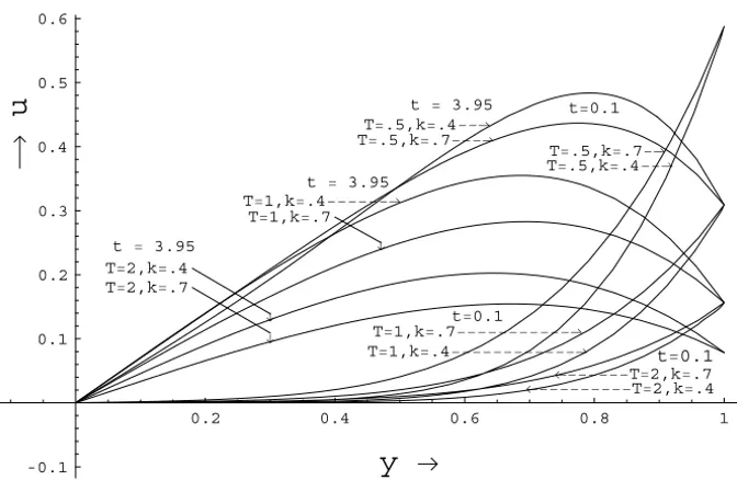
Figure 4 – Effect of the elasticity(k)on the fluid velocity for different values of time period(T)whenM =1.0.
0.2 0.4 0.6 0.8 1
-0.1 0.1 0.2 0.3 0.4 0.5 0.6
t 0.1T 2,M 0 T 2,M 1 t 0.1
T 1,M 0 T 1,M 1
t 0.1
T .5,M 1 T .5,M 0 t 3.95
T .5,M 0 T .5,M 1 t 3.95
T 1,M 0 T 1,M 1
t 3.95
T 2,M 1 T 2,M 0
u
y
(T) while Figure 5 reflects the enhancement of damping effect on the flows produced by the magnetic field with the increase of time period (T). It is to be mentioned here that in all the numerical calculations mentioned above the distance between the plates is taken as d = 1 and the non-zero values of the various dimensionless parameters M, T, t, k and d are taken arbitrarily just to test the methodology.
The fluctuations of the skin-friction with time on the lower and the upper plate are shown in Figures 6(a,b,c) and 7(a,b,c) respectively for different arbi-trary non-zerovalues of M,kandT. The results are also presented in Tables 3 and 4. It is noticed that the amplitude of skin-friction increases with the mag-netic field at the upper plate and diminishes with the same at the lower plate. Additionally, the effect of the elasticity(k)on the skin-friction decreases with the increase of the magnetic field at the lower plate while a reverse effect is found at the upper plate. In general, for fixed values of M and T the ampli-tude of skin-friction at the lower plate increases with elastic parameter(k)when the flow is developing and decreases with the same when the flow is retarding. A similar effect is also observed on the upper plate. Finally, the skin-friction on the plates corresponding to hydrodynamic situation are represented by the curves M = 0, k = 1 in Figures 6(a,b,c) and 7(a,b,c). It appears from these figures that the amplitude of skin-friction at the lower plate due to viscoelastic fluids remains always less than its classical value while at the upper plate no such definite conclusion can be made.
6 Conclusion
t T M k/y 0.0 0.125 0.25 0.375 0.5 0.625 0.75 0.875 1.0 0.4 0.0 0.0008 0.0031 0.0105 0.0309 0.0805 0.1860 0.3830 0.7071 0.0 0.7 0.0 0.0059 0.0160 0.0360 0.0744 0.1435 0.2595 0.4408 0.7071 1.0 0.0 0.0137 0.0327 0.0631 0.1124 0.1900 0.3068 0.4747 0.7071 0.4 0.0 0.0007 0.0029 0.0097 0.0289 0.0762 0.1785 0.3742 0.7071 0.5 1.0 0.7 0.0 0.0055 0.0149 0.0337 0.0702 0.1370 0.2509 0.4328 0.7071 1.0 0.0 0.0128 0.0307 0.0595 0.1069 0.1824 0.2980 0.4673 0.7071 0.4 0.0 0.0001 0.0004 0.0018 0.0067 0.0234 0.0767 0.2382 0.7071 5.0 0.7 0.0 0.0010 0.0029 0.0080 0.0209 0.0524 0.1276 0.3031 0.7071 1.0 0.0 0.0027 0.0073 0.0168 0.0370 0.0792 0.1665 0.3448 0.7071 0.4 0.0 0.0004 0.0016 0.0052 0.0156 0.0409 0.0958 0.2011 0.3827 0.0 0.7 0.0 0.0030 0.0080 0.0181 0.0378 0.0736 0.1348 0.2328 0.3827 1.0 0.0 0.0069 0.0165 0.0320 0.0575 0.0981 0.1602 0.2514 0.3827 0.4 0.0 0.0004 0.0014 0.0048 0.0146 0.0387 0.0920 0.1966 0.3827 0.125 1.0 1.0 0.7 0.0 0.0027 0.0074 0.0170 0.0357 0.0703 0.1304 0.2286 0.3827 1.0 0.0 0.0064 0.0155 0.0302 0.0547 0.0942 0.1557 0.2476 0.3827 0.4 0.0 0.0001 0.0002 0.0009 0.0034 0.0120 0.0399 0.1259 0.3827 5.0 0.7 0.0 0.0005 0.0015 0.0041 0.0107 0.0272 0.0669 0.1610 0.3827 1.0 0.0 0.0014 0.0037 0.0086 0.0191 0.0413 0.0877 0.1836 0.3827 0.4 0.0 0.0002 0.0007 0.0025 0.0076 0.0202 0.0477 0.1010 0.1950 0.0 0.7 0.0 0.0014 0.0039 0.0089 0.0187 0.0366 0.0674 0.1170 0.1950 1.0 0.0 0.0034 0.0081 0.0158 0.0285 0.0488 0.0802 0.1265 0.1950 0.4 0.0 0.0002 0.0007 0.0024 0.0072 0.0192 0.0458 0.0987 0.1950 2.0 1.0 0.7 0.0 0.0013 0.0036 0.0083 0.0176 0.0350 0.0652 0.1150 0.1950 1.0 0.0 0.0032 0.0076 0.0149 0.0271 0.0469 0.0779 0.1246 0.1950 0.4 0.0 0.0 0.0001 0.0004 0.0017 0.0060 0.0200 0.0634 0.1950 5.0 0.7 0.0 0.0002 0.0007 0.0020 0.0053 0.0136 0.0335 0.0811 0.1950 1.0 0.0 0.0007 0.0018 0.0043 0.0095 0.0207 0.0440 0.0926 0.1950
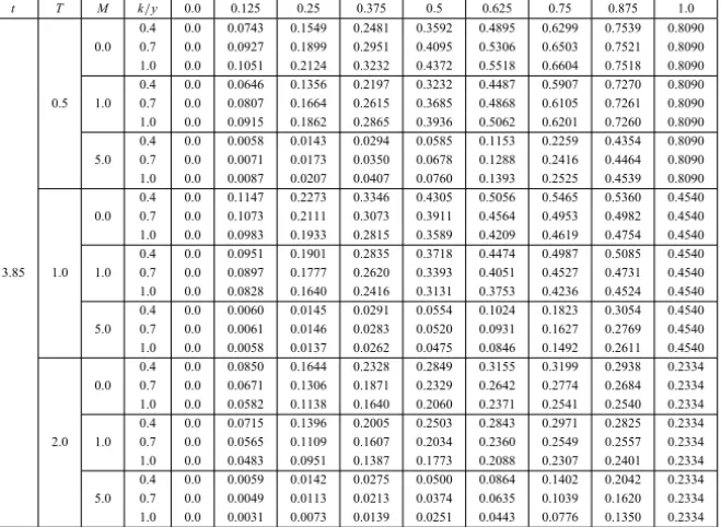
Table 1 – The fluid velocityucorresponding to developing flow for different values ofT,M,k.
t T M k/y 0.0 0.125 0.25 0.375 0.5 0.625 0.75 0.875 1.0 0.4 0.0 0.0743 0.1549 0.2481 0.3592 0.4895 0.6299 0.7539 0.8090 0.0 0.7 0.0 0.0927 0.1899 0.2951 0.4095 0.5306 0.6503 0.7521 0.8090 1.0 0.0 0.1051 0.2124 0.3232 0.4372 0.5518 0.6604 0.7518 0.8090 0.4 0.0 0.0646 0.1356 0.2197 0.3232 0.4487 0.5907 0.7270 0.8090 0.5 1.0 0.7 0.0 0.0807 0.1664 0.2615 0.3685 0.4868 0.6105 0.7261 0.8090 1.0 0.0 0.0915 0.1862 0.2865 0.3936 0.5062 0.6201 0.7260 0.8090 0.4 0.0 0.0058 0.0143 0.0294 0.0585 0.1153 0.2259 0.4354 0.8090 5.0 0.7 0.0 0.0071 0.0173 0.0350 0.0678 0.1288 0.2416 0.4464 0.8090 1.0 0.0 0.0087 0.0207 0.0407 0.0760 0.1393 0.2525 0.4539 0.8090 0.4 0.0 0.1147 0.2273 0.3346 0.4305 0.5056 0.5465 0.5360 0.4540 0.0 0.7 0.0 0.1073 0.2111 0.3073 0.3911 0.4564 0.4953 0.4982 0.4540 1.0 0.0 0.0983 0.1933 0.2815 0.3589 0.4209 0.4619 0.4754 0.4540 0.4 0.0 0.0951 0.1901 0.2835 0.3718 0.4474 0.4987 0.5085 0.4540 3.85 1.0 1.0 0.7 0.0 0.0897 0.1777 0.2620 0.3393 0.4051 0.4527 0.4731 0.4540 1.0 0.0 0.0828 0.1640 0.2416 0.3131 0.3753 0.4236 0.4524 0.4540 0.4 0.0 0.0060 0.0145 0.0291 0.0554 0.1024 0.1823 0.3054 0.4540 5.0 0.7 0.0 0.0061 0.0146 0.0283 0.0520 0.0931 0.1627 0.2769 0.4540 1.0 0.0 0.0058 0.0137 0.0262 0.0475 0.0846 0.1492 0.2611 0.4540 0.4 0.0 0.0850 0.1644 0.2328 0.2849 0.3155 0.3199 0.2938 0.2334 0.0 0.7 0.0 0.0671 0.1306 0.1871 0.2329 0.2642 0.2774 0.2684 0.2334 1.0 0.0 0.0582 0.1138 0.1640 0.2060 0.2371 0.2541 0.2540 0.2334 0.4 0.0 0.0715 0.1396 0.2005 0.2503 0.2843 0.2971 0.2825 0.2334 2.0 1.0 0.7 0.0 0.0565 0.1109 0.1607 0.2034 0.2360 0.2549 0.2557 0.2334 1.0 0.0 0.0483 0.0951 0.1387 0.1773 0.2088 0.2307 0.2401 0.2334 0.4 0.0 0.0059 0.0142 0.0275 0.0500 0.0864 0.1402 0.2042 0.2334 5.0 0.7 0.0 0.0049 0.0113 0.0213 0.0374 0.0635 0.1039 0.1620 0.2334 1.0 0.0 0.0031 0.0073 0.0139 0.0251 0.0443 0.0776 0.1350 0.2334
T M k/t 0.0 0.2 0.4 0.6 0.8 1.0 1.2 1.4 1.6 1.8 2.0 0.4 0.0 0.024 0.249 0.411 0.421 0.556 0.508 0.557 0.598 0.536 0.632 0.0 0.7 0.0 0.150 0.572 0.443 0.547 0.665 0.453 0.706 0.520 0.602 0.708 1.0 0.0 0.441 0.929 0.452 0.806 0.747 0.521 0.896 0.411 0.770 0.718 0.4 0.0 0.021 0.204 0.319 0.326 0.440 0.400 0.456 0.488 0.446 0.530 0.5 1.0 0.7 0.0 0.135 0.486 0.351 0.459 0.550 0.374 0.598 0.425 0.514 0.594 1.0 0.0 0.389 0.797 0.359 0.695 0.622 0.442 0.768 0.327 0.669 0.600 0.4 0.0 0.001 0.006 0.007 0.010 0.014 0.015 0.020 0.021 0.024 0.027 5.0 0.7 0.0 0.014 0.026 0.013 0.031 0.027 0.028 0.038 0.024 0.041 0.035 1.0 0.0 0.046 0.060 0.015 0.065 0.032 0.046 0.060 0.014 0.065 0.032 0.4 0.0 0.012 0.151 0.388 0.581 0.613 0.472 0.435 0.558 0.685 0.684 0.0 0.7 0.0 0.078 0.396 0.682 0.753 0.559 0.323 0.512 0.754 0.806 0.600 1.0 0.0 0.238 0.700 0.971 0.895 0.492 0.291 0.682 0.948 0.875 0.476 0.4 0.0 0.011 0.125 0.310 0.453 0.473 0.368 0.360 0.469 0.568 0.560 1.0 1.0 0.7 0.0 0.071 0.339 0.570 0.618 0.449 0.265 0.441 0.641 0.673 0.493 1.0 0.0 0.208 0.608 0.831 0.753 0.398 0.243 0.594 0.814 0.739 0.386 0.4 0.0 0.001 0.004 0.008 0.012 0.014 0.015 0.018 0.022 0.026 0.027 5.0 0.7 0.0 0.007 0.021 0.031 0.031 0.022 0.021 0.034 0.041 0.040 0.030 1.0 0.0 0.025 0.057 0.067 0.052 0.017 0.025 0.057 0.067 0.052 0.017 0.4 0.0 0.006 0.079 0.224 0.400 0.570 0.702 0.776 0.781 0.716 0.584 0.0 0.7 0.0 0.039 0.213 0.428 0.624 0.771 0.850 0.850 0.772 0.621 0.413 1.0 0.0 0.119 0.382 0.641 0.843 0.966 0.995 0.929 0.772 0.512 0.258 0.4 0.0 0.005 0.065 0.180 0.316 0.447 0.552 0.614 0.625 0.582 0.488 2.0 1.0 0.7 0.0 0.035 0.183 0.360 0.520 0.639 0.703 0.703 0.640 0.516 0.346 1.0 0.0 0.104 0.334 0.554 0.724 0.825 0.846 0.786 0.650 0.450 0.207 0.4 0.0 0.0 0.002 0.005 0.008 0.013 0.017 0.022 0.025 0.027 0.028 5.0 0.7 0.0 0.004 0.012 0.021 0.029 0.036 0.040 0.041 0.039 0.034 0.027 1.0 0.0 0.013 0.032 0.049 0.061 0.067 0.066 0.059 0.046 0.029 0.008
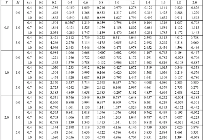
Table 3 – The skin-frictionτ0at the lower platey=0 for different values ofT,M,k.
T M k/t 0.0 0.2 0.4 0.6 0.8 1.0 1.2 1.4 1.6 1.8 2.0
0.4 0.0 1.389 -0.150 1.059 0.716 -0.979 1.278 -0.129 1.141 0.820 -0.876 0.0 0.7 0.0 1.698 -0.345 1.368 0.833 -1.317 1.592 -0.316 1.425 0.888 -1.270 1.0 0.0 1.862 -0.540 1.583 0.869 -1.627 1.794 -0.497 1.632 0.911 -1.593 0.4 0.0 1.504 0.0307 1.219 0.959 -0.796 1.498 0.104 1.316 1.057 -0.708 0.5 1.0 0.7 0.0 1.844 -0.134 1.525 1.079 -1.158 1.802 -0.084 1.584 1.132 -1.113 1.0 0.0 2.054 -0.289 1.747 1.139 -1.470 2.013 -0.251 1.785 1.172 -1.443 0.4 0.0 3.421 2.112 2.739 3.722 0.511 4.044 2.593 3.113 4.012 0.738 5.0 0.7 0.0 4.266 2.270 3.114 4.175 -0.055 4.542 2.492 3.292 4.318 0.060 1.0 0.0 4.966 2.443 3.446 4.590 -0.471 4.978 2.452 3.454 4.596 -0.466 0.4 0.0 0.984 1.066 0.668 -0.007 -0.602 0.906 1.107 0.763 0.104 -0.497 0.0 0.7 0.0 1.221 1.246 0.722 -0.083 -0.752 1.172 1.291 0.782 -0.028 -0.706 1.0 0.0 1.363 1.379 0.788 -0.132 -0.906 1.317 1.403 0.816 -0.108 -0.887 0.4 0.0 1.050 1.233 0.912 0.246 -0.427 1.072 1.319 1.015 0.346 -0.338 1.0 1.0 0.7 0.0 1.304 1.449 0.995 0.166 -0.620 1.306 1.508 1.056 0.219 -0.576 1.0 0.0 1.474 1.620 1.087 0.119 -0.795 1.447 1.641 1.109 0.137 -0.780 0.4 0.0 2.170 3.537 3.714 2.598 0.657 2.780 4.008 4.080 2.883 0.880 5.0 0.7 0.0 2.725 4.242 4.204 2.612 0.160 2.997 4.461 4.379 2.753 0.273 1.0 0.0 3.183 4.849 4.658 2.683 -0.207 3.192 4.857 4.664 2.688 -0.202 0.4 0.0 0.531 0.746 0.849 0.859 0.787 0.648 0.457 0.232 -0.004 -0.183 0.0 0.7 0.0 0.660 0.890 0.994 0.997 0.909 0.738 0.501 0.219 -0.079 -0.301 1.0 0.0 0.740 1.001 1.130 1.141 1.037 0.829 0.538 0.193 -0.172 -0.442 0.4 0.0 0.565 0.841 1.018 1.096 1.076 0.961 0.762 0.499 0.195 -0.072 2.0 1.0 0.7 0.0 0.703 1.006 1.187 1.254 1.205 1.044 0.787 0.457 0.087 -0.223 1.0 0.0 0.798 1.139 1.345 1.413 1.341 1.136 0.818 0.419 -0.021 -0.382 0.4 0.0 1.144 2.198 3.119 3.798 4.156 4.146 3.759 3.029 2.020 0.879 5.0 0.7 0.0 1.438 2.661 3.656 4.322 4.586 4.418 3.833 2.884 1.661 0.351 1.0 0.0 1.680 3.056 4.130 4.798 4.996 4.704 3.951 2.810 1.394 -0.078
0.5 1 1.5 2 2.5 0.2
0.4 0.6 0.8
M 0,k 1.0
M 1,k 1.0 M 1,k 0.7 M 1,k 0.4
M 5,k 1.0 M 5,k 0.7 M 5,k 0.4
t
0
Figure 6(a) – Effects of the magnetic field(M)and the elasticity(k)on the skin-friction at the lower platey=0 whenT =0.5.
0.5 1 1.5 2 2.5
0.2 0.4 0.6 0.8
M 0,k 1.0
M 1,k 1.0 M 1,k 0.7 M 1,k 0.4
M 5,k 1.0 M 5,k 0.7 M 5,k 0.4
t
0
0.5 1 1.5 2 2.5 0.2
0.4 0.6 0.8 1
M 0,k 1.0
M 1,k 0.4 M 1,k 0.7 M 1,k 1.0
M 5,k 0.4 M 5,k 0.7 M 5,k 1.0
t
0
Figure 6(c) – Effects of the magnetic field(M)and the elasticity(k)on the skin-friction at the lower platey=0 whenT =2.0.
0.2 0.4 0.6 0.8 1
5 10 15 20
1
t
k
0
.
4
k
0
.
7
k
1
.
0
M
1
0
k 0.4 k 0.7 k 1.0
M 20
k
.
4
k
.
7
k
1
. M
5
M 0.0,k 1.0 M 1 k 0.4
k 0.7 k 1.0
0.5 1 1.5 2 5
10 15 20
1
t
M 0.0,k 1.0 k 0.4
k 0.7 k 1.0
M 20
k
0
.
4
k
0
.
7
k
1
.
0
M
1
0
k
0
.
4
k
0
.
7
k
1
.
0
M
5
k 0.4 k 0.7
k 1.0 M 1
Figure 7(b) – Effects of the magnetic field (M) and the elasticity(k)on the skin-friction at the upper platey=dwhenT =1.0.
1 2 3 4
2 4 6 8 10
1
t
M 0.0,k 1.0 k 0.4
k 0.7 k 1.0
M 10
k
0
.
4
k
0
.
7
k
1
.
0
M
5
k
0
.
4
k
0
.
7
k
1
.
0
M
1
unsteady motion differ significantly. As a result, the flow phenomena discussed in [13] is not the same as that of the present analysis. Moreover, the fluid flow, generated by tooth pulses as discussed in [13], is supposed to have importance in white dwarf asteroseismology [14] and acoustic and acousto-gravity wave pulses caused by sources of seismic origin [15]. On the other hand, the flow pro-duced by rectified sine pulses as considered in the present paper has applications in planetary tides and sunspot cycles [16], peristaltic transport of a particle-fluid suspension [17], pulsed microwave plasma etching of polymers [18], adaptive noise reduction for pulmonary artery blood pressure [19] and Wavelab’s elevated frequency resolution to music therapy [20]. Several other applications of tooth pulses and rectified sine pulses in physical problems may also be found in the literature as substantial references.
We further observe that the skin-friction on the lower plate appears to have symmetrical peaks for all values of the magnetic fieldMwhile the skin-friction on the upper plate contains non-symmetrical peaks particularly at small values ofMdue to the appearance of negative skin-friction in such a stage. However, with the increase of the strength of the magnetic field the values of the negative skin-friction on the upper plate, developed during its retarding motion, goes on diminishing. This leads to the restoration of symmetrical peaks of skin-friction on the upper plate for large values of M when skin-friction remains always positive (Figures 7(a,b,c)). This is a consequence of the effect of magnetic field in presence of pulsation.
Finally, we add that in order to produce a four digit accuracy in Tables 1 to 4, we have considered first 100 terms of m and n series. For the sake of convenience in numerical calculation two different expansion indexes m and n are considered in Eq.(4.13) and Eq.(4.27). However one can take only one expansion index to represent both the series.
Acknowledgement. The authors are very much grateful to the referees for providing many helpful suggestions to improve the paper in its present form.
Appendix
Then we have
St =
∞
X
n=1
Wn′(0)e m1t
−em2t
m1−m2 +Wn(0) m1em2t
−m2em1t m1−m2
sinnπy d
Now,
Wn′(0) = 8n(−1)
n
d2 Im
∞ X
m=1
βm
{(2m)2−1}L2
m+n
2π2
d2
= 8n(−1)
n
d2 Im
∞ X
m=1
βm(1+iβmk)
{(2m)2−1}(s1−iβm)(s2−iβm)
= 8n(−1)
n
d2 Im
∞ X
m=1 βm
{(2m)2−1}
−1s+ks1
1−s2 ∙
1
s1−iβm +
1+ks2
s1−s2 ∙
1
s2−iβm
= 8n(−1)
n
d2
∞ X
m=1 βm
{(2m)2−1}
(
−1s+ks1
1−s2 ∙ βm
s12+βm2 +
1+ks2
s1−s2 ∙
βm
s22+βm2
)
= 8n(−1)
n
d2
∞ X
m=1 (
−1+ks1
s1−s2 ∙
βm2
{(2m)2−1} s12+βm2
+1s+ks2
1−s2 ∙
βm2
{(2m)2−1}s22+β2m
)
= 8n(−1)
n d2 ∞ X
m=1
−1+ks1
s1−s2 ∙
(2m)2π2
T2{(2m)2−1}ns12+ (2m)2π2
T2 o
+
∞ X
m=1
1+ks2
s1−s2 ∙
(2m)2π2
T2{(2m)2−1}ns22+(2m)2π2
T2 o
= 8n(−1)
n d2 ∞ X
m=1
−1s+ks1
1−s2
1
(2m)2−1−
s12T2
{(2m)2−1}ns2
1T2+(2m)2π2 o + ∞ X
m=1 1
+ks2
s1−s2
1
(2m)2−1−
s22T2
{(2m)2−1}ns2
2T2+(2m)2π2 o
= 8n(−1)
n
d2
∞ X
m=1
1+ks2
s1−s2 −
1+ks1
s1−s2
1
+1+ks1
s1−s2
(
1
(2m)2−1−
π2
s21T2+(2m)2π2
)
s12T2
s12T2+π2
−1s+ks2
1−s2 (
1
(2m)2−1−
π2
s22T2+(2m)2π2
)
s22T2
s22T2+π2
#
= 8n(−1)
n d2 ∞ X
m=1
−k
(2m)2−1+
1
(2m)2−1 (
1+ks1
s1−s2
s12T2
s12T2+π2
−1s+ks2
1−s2
s22T2
s22T2+π2
)
−1s+ks1
1−s2
π2s12T2
s12T2+π2
∞ X
m=1
1
s21T2+(2m)2π2
+1+ks2
s1−s2
π2s22T2
s22T2+π2
∞ X
m=1
1
s22T2+(2m)2π2
= 8n(−1)
n d2 " −k 2 + 1 2 (
1+ks1
s1−s2
s12T2
s12T2+π2−
1+ks2
s1−s2
s22T2
s22T2+π2
)
− 1s+ks1
1−s2
π2s12T2
s12T2+π2
1 4s1T
∞ X
m=1
2s1T 2
s1T
2 2
+m2π2
+1s+ks2
1−s2
π2s22T2
s22T2+π2
1 4s2T
∞ X
m=1
2s2T 2 s 2T 2 2
+m2π2
= 8n(−1)
n d2 " −k 2 + 1 2 (
1+ks1
s1−s2
s21T2
s12T2+π2−
1+ks2
s1−s2
s22T2
s22T2+π2
)
− 1+ks1
4(s1−s2)
π2s1T
s12T2+π2
coth
s1T
2
− 2
s1T
+4(1s+ks2
1−s2)
π2s2T
s22T2+π2
coth s 2T 2
− s2
2T #
= 8n(−1)
n d2 −k 2 + 1 2
1+ks1
s1−s2 −
1+ks2
s1−s2
− 1
2
(
1+ks1
s1−s2
π2
s12T2+π2 −
1+ks2
s1−s2
π2
s22T2+π2
)
− 4(1s+ks1
1−s2)
π2s1T
s12T2+π2coth
s1T
2
+4(1s+ks2
1−s2) π2s2T
s22T2+π2coth
s2T
2
+1 2
(
1+ks1
s1−s2
π2
s12T2+π2 −
1+ks2
s1−s2
π2
s22T2+π2
)#
= 8n(−1)
n d2 " −k 2 + k 2−
1+ks1
4(s1−s2)
π2s1T
s12T2+π2coth
s 1T
2
+4(1s+ks2
1−s2)
π2s2T
s22T2+π2coth
s 2T
2
#
= 2n(−1)
n+1
d2
"
1+ks1
s1−s2
π2s1T
s12T2+π2coth
s1T
2
−1s+ks2
1−s2
π2s2T
s22T2+π2coth
s2T
2
#
Again,
Wn(0) =
4n(−1)n
d2
1
M2+n2π2
d2
−2 Re
∞ X
m=1
1
{(2m)2−1}L2
m+n
2π2
d2
= 4n(−1)
n
d2
1
M2+n2π2
d2
−2 Re
∞ X
m=1
(1+iβmk)
{(2m)2−1}(s1−iβm)(s2−iβm)
= 4n(−1)
n
d2
1
M2+n2π2
d2
−2 Re
∞ X
m=1
1
(2m)2−1∙
−1+ks1
s1−s2 ∙
1
(s1−iβm)
+
1+ks2
s1−s2
∙ 1
(s2−iβm)
= 4n(−1)
n
d2
1
M2+n2π2
d2
−2 Re
∞ X
m=1
1
(2m)2−1∙
−1+ks1
s1−s2 ∙
s1+iβm
s12+βm2
+
1
+ks2
s1−s2
∙ s2+iβm
s22+βm2
)#
= 4n(−1)
n
d2
1
M2+n2π2
d2
−2
∞ X
m=1 (
−1s+ks1
1−s2 ∙
s1
{(2m)2−1} s2
1+βm2
+
1+ks2
s1−s2
∙ s2
{(2m)2−1} s2
2+βm2
= 4n(−1) n d2 1
M2+n2π2
d2
−2
∞ X
m=1
−1+ks1
s1−s2 ∙
s1T2
{(2m)2−1}ns12T2+(2m)2π2o
+1+ks2
s1−s2 ∙
s2T2
{(2m)2−1}ns22T2+(2m)2π2o
= 4n(−1)
n
d2
1
M2+n2π2
d2
−2
∞ X
m=1
−
1+ks1
s1−s2
×
(
1
(2m)2−1−
π2
s21T2+(2m)2π2
)
s1T2
s12T2+π2
+
1
+ks2
s1−s2
∙
(
1
(2m)2−1−
π2
s22T2+(2m)2π2
)
s2T2
s22T2+π2
#
= 4n(−1)
n
d2
1
M2+n2π2
d2
+
(
1+ks1
s1−s2 ∙
s1T2
s12T2+π2−
1+ks2
s1−s2 ∙
s2T2
s22T2+π2
)
−2
1
+ks1
s1−s2
∙ s1T
2π2
s12T2+π2
∞ X
m=1
1
s12T2+(2m)2π2
+2
1+ks2
s1−s2
∙ s2T
2π2
s22T2+π2
∞ X
m=1
1
s22T2+(2m)2π2
= 4n(−1)
n
d2
1
M2+n2π2
d2
+
(
1+ks1
s1−s2 ∙
s1T2
s12T2+π2−
1+ks2
s1−s2 ∙
s2T2
s22T2+π2
)
−2
1+ks1
s1−s2
∙ s1T
2π2
s12T2+π2∙
1 4s1T
∞ X
m=1
2s1T 2 s 1T 2 2
+m2π2
+2
1+ks2
s1−s2
∙ s2T
2π2
s22T2+π2∙
1 4s2T
∞ X
m=1
2s2T 2 s 2T 2 2
+m2π2
= 4n(−1)
n
d2
1
M2+n2π2
d2
+
(
1+ks1
s1−s2 ∙
s1T2
s12T2+π2−
1+ks2
s1−s2 ∙
s2T2
s22T2+π2
)
− 1
2s1T ∙
1+ks1
s1−s2
∙ s1T
2π2
s12T2+π2
coth
s1T
2
− 2
s1T
+ 1 2s2T
1+ks2
s1−s2
∙ s2T
2π2
s22T2+π2
coth
s2T
2
− 2
s2T
#
= 4n(−1)
n
d2
1
M2+n2π2
d2
+
(
1+ks1
s1−s2 ∙
s1T2
s12T2+π2−
1+ks2
s1−s2 ∙
s2T2
s22T2+π2
)
−1
2∙
1+ks1
s1−s2
∙ π
2T
s12T2+π2coth
s1T
2
+s1
1∙
1+ks1
s1−s2
∙ π
2
s12T2+π2
+1
2∙
1+ks2
s1−s2
∙ π
2T
s22T2+π2coth
s2T
2
− 1
s2
1+ks2
s1−s2
∙ π
2
s22T2+π2
#
= 4n(−1)
n
d2
1
s1s2+
1
+ks1
s1(s1−s2)−
1+ks2
s2(s1−s2)
−1
2
1+ks1
s1−s2
∙ π
2T
s12T2+π2coth
s1T
2
+12
1
+ks2
s1−s2
∙ π
2T
s22T2+π2coth
s 2T
2
#
= 4n(−1)
n
d2
"
1
s1s2−
1
s1s2 −
1 2
1
+ks1
s1−s2
∙ π
2T
s12T2+π2coth
s 1T
2
+12
1+ks2
s1−s2
∙ π
2T
s22T2+π2coth
s2T
2
#
= 2n(−1)
n+1
d2
"
1+ks1
s1−s2
∙ π
2T
s12T2+π2coth
s1T
2
−
1+ks2
s1−s2
∙ π
2T
s22T2+π2coth
s2T
2
#
Therefore,
St =
∞ X
n=1
Wn′(0)e
m1t−em2t
m1−m2 +
Wn(0)
m1em2t−m2em1t
m1−m2
sinnπy
d
St =
∞ X
n=1
Wn′(0)e
s1t−es2t
s1−s2 +
Wn(0)
s1es2t−s2es1t
s1−s2
sinnπy
=
∞ X
n=1 "(
Wn′(0)−s2Wn(0)
s1−s2
)
es1t+
(
s1Wn(0)−Wn′(0)
s1−s2
)
es2t #
sinnπy
d
=
∞ X
n=1 "
2n(−1)n+1
d2
(
1+ks1
s1−s2 ∙
π2T
s12T2+π2∙coth
s1T
2
∙es1t
−1s+ks2
1−s2 ∙ π2T
s22T2+π2 ∙coth
s 2T
2
∙es2t
)#
sinnπy
d
=
∞ X
n=1 "
2n(−1)n+1
d2
(
π2T1+ks1
s1−s2coth
s 1T
2
∙ e
s1t
s21T2+π2
−π2T1+ks2
s1−s2
coth
s2T
2
∙ e
s2t
s22T2+π2
)#
sinnπy
d
=
∞ X
n=1
2n(−1)n+1
d2 π2 T
coths1T 2
a1+(1+bks1
1)2
∙ e
s1t
s12+π2
T2 +π 2 T coth s2T
2
a1+ b1
(1+ks2)2
∙ e
s2t
s22+π2
T2 sin
nπy
d
= −2π
2
T d2
∞ X
n=1
n(−1) n
coths1T 2
a1+(1 b1
+ks1)2
∙ e
s1t
s12+ π2
T2
+π
2
T
coths2T 2
a1+ (1+bks1
2)2
∙ e
s2t
s22+π2
T2 sin
nπy
d
= −2π
2
T d2
∞ X
n=1
n(−1)n∙D∙sinnπy
d
where
a1= 1
k, b1=
M2−1 k
(1−k) and D= D1+D2,
Dj =
esjtcoth
s jT 2 s2 j + π2
T2 a1+
b1
(1+ksj)2
, j =1,2.
Thus the two solutions (4.13) and (4.25) are the same for all values of y, k, M andt. This implies that the method of Fourier analysis which is simpler than that of Laplace transforms can be used successfully to solve similar types of problems.
REFERENCES
[1] A. Chakraborty and J. Ray,Unsteady magnetohydrodynamic Couette flow between two plates
when one of the plates is subjected to random pulses. J. Phys. Soc. Jpn.,48(1980), 1361.
[2] M.N. Makar, Magnetohydrodynamic flow between two plates when one of the plates is
subjected to tooth pulses. Acta Phys. Pol.,A71(1987), 995.
[3] A.R. Bestman and F.I. Njoku, On hydromagnetic channel flow induced by tooth pulses. Preprint IC/88/10, Miramare-Trieste, (1988).
[4] A.K. Ghosh and L. Debnath,On hydromagnetic pulsatile flow of a two-phase fluid. ZAMM,
76(2) (1996), 121.
[5] N. Datta, D.C. Dalal and S.K. Misra, Unsteady heat transfer to pulsatile flow of a dusty
viscous incompressible fluid in a channel. Int. J. Heat Mass Transfer,36(7) (1993), 1783.
[6] N. Datta and D.C. Dalal,Pulsatile flow and heat transfer of a dusty fluid through an infinitely
long annular pipe. Int. Multiphase Flow,21(3) (1995), 515.
[7] T. Hayat, A.M. Siddiqui and S. Asghar, Some simple flows of an Oldroyd-B fluid. Int. J. Engg. Sci.,39(2001), 135.
[8] S. Asghar, S. Parveen, S. Hanif, A.M. Siddiqui and T. Hayat, Hall effects on the unsteady
hydromagnetic flows of an Oldroyd-B fluid. Int. J. Engg. Sci.,41(2003), 609.
[9] T. Hayat, S. Nadeem and S. Asghar, Hydromagnetic Couette flow of an Oldroyd-B fluid in a
rotating system. Int. J. Engg. Sci.,42(2004), 65.
[10] E.F. El-Shehawey, E.M.E. Elbarbary, N.A.S. Afifi and M. Elshahed,MHD flow of an
Elastico-Viscous fluid under periodic body acceleration. Int. J. Math. and Math. Sci.,23(11) (2000),
795.
[11] V.M. Soundalgekar,On the flow of an electrically conducting, incompressible fluid near an
accelerated plate in the presence of a parallel plate, under transverse magnetic field. Proc.
Indian Acad. Sci.,A65(1967), 179.
[12] H.S. Carslaw and J.C. Jaeger,Operational Methods in Applied Mathematics. Dover Publi-cation, Inc., New York (1963).
[13] A.K. Ghosh and P. Sana,On hydromagnetic channel flow of an Oldroyd-B fluid induced by
tooth pulses. Magnetohydrodynamics,44(3) (2008), 325–340.
[15] S.V. Koshevaya, V.V. Grimalsky, J. Siqueiros-Alatorre, R. Perez-Enriquez and A.N. Kot-sarenko, Acoustic and Acousto-Gravity Wave Pulses Caused by Sources of Seismic Origin. Physica Scripta,70(2004), 72–78.
[16] J.J. Condon and R.R. Schmidt,Planetary tides and sunspot cycles. Solar Physics,42(1975), 529–532.
[17] K.S. Mekheimer and Y. Abdelmaboud, Peristaltic transport of a particle-fluid suspension
through a uniform and non-uniform annulus. Applied Bionics and Biomechanics,5(2), (June
2008), 47–57.
[18] T.H. Lin, M. Belser and Yonhua Tzeng, Pulsed microwave plasma etching of polymers
in Oxygen and Nitrogen for microelectronic applications. IEEE, Transaction on Plasma
Science,16(6), (Dec. 1998), 631–637.
[19] Kang-Ping Lin and W.H. Chang,Adaptive noise reduction for pulmonary artery blood pres-sure. Engineering in medicine and Biology Society, Proceedings of the Annual International Conference of the IEEE,Vol. I, (1988), 82–83.