Enda Dimitri V. Bigarella
[email protected] Embraer S.A. Av. Brigadeiro Faria Lima, 2170 S ˜ao Jos ´e dos Campos 12227-901 SP, Brazil
Jo ˜ao Luiz F. Azevedo
[email protected] Instituto de Aeron´autica e Espac¸o Departamento de Ci ˆencia e Tecnologia Aeroespacial DCTA/IAE/ALA S ˜ao Jos ´e dos Campos 12228-903 SP, Brazil
A Study of Convective Flux Schemes for
Aerospace Flows
This paper presents the effects of some convective flux computation schemes on boundary layer and shocked flow solutions. Second-order accurate centered and upwind convective flux computation schemes are discussed. The centered Jameson scheme, plus explicitly added artificial dissipation terms are considered. Three artificial dissipation models, namely a scalar and a matrix version of a switched model, and the CUSP scheme are available. Some implementation options regarding these methods are proposed and addressed in the paper. For the upwind option, the Roe flux-difference splitting scheme is used. The CUSP and Roe schemes require property reconstructions to achieve second-order accuracy in space. A multidimensional limited MUSCL interpolation method is used to perform property reconstruction. Extended multidimensional limiter formulation and implementation are here proposed and verified. Theoretical flow solutions are used in order to provide a representative testbed for the current study. It is observed that explicitly added artificial dissipation terms of the centered scheme may nonphysically modify the numerical solution, whereas upwind schemes seem to better represent the flow structure. Keywords: CFD, numerical flux schemes, compressible viscous flows, compressible inviscid flows
Introduction
The paper reports recent improvements on a finite volume method for 3-D unstructured meshes developed by the CFD group at Instituto de Aeron´autica e Espac¸o (IAE). Flow phenomena typical of aerospace applications are usually associated with transonic and supersonic shock waves and high-Reynolds number boundary layers. The correct computation of such flow phenomena is of paramount importance for the representativeness of numerical simulations for high Mach and Reynolds-number flight conditions, since they are decisive for the final aerodynamic data important for engineering purposes. The numerical modeling of these flow features, through flux computation schemes, must be representative of the physics of these phenomena, as well as numerically adequate in terms of robustness and costs. In light of that, the paper addresses several flux computation schemes suitable for the typical aerospace applications of IAE.
Second-order accurate centered- (Jameson, Schmidt and Turkel, 1981) and upwind flux-difference splitting (Roe, 1981) schemes are considered here. In the centered case, explicit addition of artificial dissipation terms is required to control nonlinear instabilities in the numerical solution. For computation of these terms in the current work, both the scalar and the matrix versions of a switched second-and fourth-difference scheme are considered (Mavriplis, 1990; Turkel and Vatsa, 1994). The Convective-Upwind Split-Pressure (CUSP) artificial dissipation model (Jameson, 1995a; Jameson, 1995b) is also considered in the centered scheme case. Some implementation options are proposed and discussed in the paper, in terms of computational effort and numerical solution quality.
The CUSP and the Roe upwind schemes require special treatment of properties in the control-volume faces to achieve 2nd-order accuracy in space. The multidimensional, limited, MUSCL (van Leer, 1979) reconstruction scheme of Barth and Jespersen (1989) is adopted here. This limiter formulation is here addressed, and an extension for this formulation is proposed and assessed in the paper. A computationally cheap and robust integration of the limited MUSCL-reconstructed schemes is also proposed, which allows for large computational resource savings while maintaining the expected level of accuracy.
Paper received 27 July 2009. Paper accepted 29 November 2011
Technical Editor: Eduardo Belo
Inviscid flows for a 1-D shock tube and the Boeing A4 supercritical airfoil (Nishimura, 1992) configurations are considered in order to address the flux computation schemes for shock wave capturing. A mesh refinement study is performed for the airfoil case in order to assess the dependency of the numerical schemes with grid density and topology.
Subsonic laminar flows over a flat plate address the effects of the numerical flux schemes in boundary layer flows. It is known that flux schemes may have influence in such flow solutions, as reported by Swanson, Radespiel and Turkel (1998), Zingg et al. (1999), Allmaras (2002), and Bigarella (2002). The present group attributes such problems to nonphysical behavior of centered flux schemes, more precisely in the explicitly added artificial dissipation model, as reported in Bigarella, Moreira and Azevedo (2004). The present paper shows conclusive results that corroborate this assertive. Mesh density and topology are also addressed for such test case. Generally, improved accuracy is obtained with the new flux computation schemes.
This section presents the motivation for the current effort. The next section presents a brief discussion on the theoretical and numerical formulations embedded in the current numerical tool. Detailed discussion on the centered schemes here considered is performed in the third section. Similar discussion is performed for the upwind and the reconstruction schemes in the fourth section. The fifth section presents the discussions on the obtained numerical results. The last section closes the work with concluding remarks from the current effort.
Nomenclature
a = speed of sound
C = convective operator
CFL = Courant-Friedrichs-Lewy number C p = pressure coefficient
D = artificial dissipation operator d = artificial dissipation term e = total energy per unit volume ei = internal energy
n f = number of faces that compose a control volume p = static pressure
Pv = viscous flux vector Pr = Prandtl number
q = heat flux vector
Q = vector of conserved properties Re = Reynolds number
S=|S| = face area
u, v, w = cartesian velocity components
v = cartesian velocity vector
V = viscous operator x, y, z = cartesian coordinates
Greek Symbols
α = angle of attack ∆t = time step
Φ = gradient ratio for limiter computation γ = ratio of specific heats
µ = dynamic viscosity coefficient ψ = control volume limiter ρ = density
τ = viscous stress tensor
Subscripts
∞ = freestream property i,m = grid control volume indices k = face index
ℓ = laminar property
L,R = interface left and right properties t = turbulent property
Superscripts
∗ = dimensional property n = time instant
Theoretical and Numerical Formulations
The flows of interest in the present context are modeled by the 3-D compressible Reynolds-averaged Navier-Stokes (RANS) equations, written in dimensionless form and assuming a perfect gas, as
∂Q
∂t +∇·(Pe−Pv) =0 ,
Q= ρ ρu ρv ρw e T . (1)
The inviscid and viscous flux vectors are given as
Pe= ρv
ρuv+p ˆıx
ρvv+p ˆıy
ρwv+p ˆız
(e+p)v
, Pv=
1 Re 0
τxiˆıi
τyiˆıi
τziˆıi
βiˆıi
. (2)
The shear-stress tensor is defined by
τi j=µℓ
∂
ui
∂xj +∂uj
∂xi
−2
3
∂um
∂xm
δi j
, (3)
where ui represents the Cartesian velocity components, and xi represents the Cartesian coordinates. The viscous force work and heat
transfer term,βi, is defined asβi=τi juj−qi, where the heat transfer component is defined as
qj=−γ
µℓ
Pr ∂(ei)
∂xj
. (4)
The molecular dynamic viscosity coefficient is computed by the Sutherland law (Anderson, 1991). The dimensionless pressure can be calculated from the perfect gas equation of state.
This set of equations is solved according to a finite volume formulation (Scalabrin, 2002). Flow equations are integrated in time by a fully explicit, 2nd-order accurate, 5-stage, Runge-Kutta time stepping scheme. An agglomeration full-multigrid scheme (FMG) is included in order to achieve better convergence rates for the simulations. More details on the theoretical and numerical formulations can be found in Bigarella, Basso and Azevedo (2004), and Bigarella and Azevedo (2005).
Centered Spatial Discretization Schemes
Centered schemes require the explicit addition of artificial dissipation terms in order to control nonlinear instabilities that may arise in the flow simulation. Several models to compute the artificial terms are included in the present numerical formulation. A description of the available models is presented in the forthcoming subsections.
Mavriplis scalar switched model (MAVR)
The centered spatial discretization of the convective fluxes, Ci, in this scheme is proposed by Jameson, Schmidt and Turkel (1981). The convective operator is calculated as the sum of the inviscid fluxes on the faces of the i-th volume as
Ci= n f
∑
k=1Pe(Qk)·Sk, Qk= 1
2(Qi+Qm), (5)
where Qiand Qmare the conserved properties in the i-th and m-th cells, respectively, that share the k-th face.
The artificial dissipation operator is built by a blend of undivided Laplacian and bi-harmonic operators. In regions of high property gradients, the bi-harmonic operator is turned off in order to avoid oscillations. In smooth regions, the undivided Laplacian operator is turned off in order to maintain 2nd order accuracy. A numerical pressure sensor is responsible for this switching between the operators. The expression for the artificial dissipation operator is given by
Di= nb
∑
k=1
1
2(Am+Ai)
h
ǫ2(Qm−Qi)−ǫ4
∇2
Qm−∇2Qi i
,
(6)
where m represents the neighbor of the i-th element, attached to the
k-th face, and nb is the total number of neighbors of the i-th control
volume. Furthermore,
∇2Q
i =
nb
∑
k=1[Qm−Qi],
ǫ2 = K2max(νi,νm),
ǫ4 = max(0,K4−ǫ2) , (7)
νi = ∑
nb
m=1|pm−pi|
∑nb
In this work, K2 and K4 are assumed equal to 1/4 and 3/256,
respectively, as recommended by Jameson, Schmidt and Turkel (1981).
The Ai matrix coefficient in Eq. (6) is replaced by a scalar coefficient (Mavriplis, 1988; Mavriplis, 1990) defined as
Ai= n f
∑
k=1[|vk·Sk|+ak|Sk|]. (8)
This formulation is constructed so as to obtain steady state solutions which are independent of the time step (Azevedo, 1992).
In the multistage Runge-Kutta time integration previously described, the artificial dissipation operator is calculated only on the first, third and fifth stages for viscous flow simulations. For the inviscid calculations, the artificial dissipation operator is calculated in the first and in the second stages only. This approach guarantees the accuracy for the numerical solution while reducing computational costs per iteration (Jameson, Schmidt and Turkel, 1981). Furthermore, the MAVR model has also been integrated into the multigrid framework. In order to achieve lower computational costs for the multigrid cycles, only the first order artificial dissipation model is used in the coarser mesh levels. This operation is achieved by not computing the bi-harmonic term in Eq. (6) and by setting ǫ2←ǫ2+ǫ4in these levels.
Matrix switched model (MATD)
The formulation for the matrix model (MATD) is similar to the previously described one for the MAVR model, except for the definition of the Aiterms. In this case, the flux Jacobian matrices, as defined in Turkel and Vatsa (1994), are used instead of the scalar term inside the summation in Eq. (8). The Aiterm, re-interpreted for the present cell-centered, face-based finite-volume framework, can be written as
Ai= n f
∑
k=1|Ak||Sk|, (9)
where
|Ak| = |λ3|I+
1
2(|λ1|+|λ2|)− |λ3|
γ−1
a2k E1+E2 !
+ 1
2ak
(|λ1| − |λ2|) [E3+ (γ−1)E4]. (10)
In this equation, the following definitions in the k-th face are used:
|λ1| = max(|vn+a|,Vnλ), |λ2| = max(|vn−a|,Vnλ),
|λ3| = max(|vn|,Vlλ), (11)
λ = |vn|+a ,
and the k subscript is dropped in order to avoid overloading the previous formulation nomenclature. In these definitions, vn is the normal velocity component, computed as vn=v·n, where the unit area vector is defined as n=S/|S|. Furthermore, in these expressions,
Vnlimits the eigenvalues associated with the nonlinear characteristic fields whereas Vlprovides a similar limiter for the linear characteristic fields. Such limiters are used near stagnation and/or sonic lines, where the eigenvalues approach zero, in order to avoid zero artificial dissipation. The values recommended for these limiters by Turkel and
Vatsa (1994), Vn=0.25 and Vl=0.025, are used in the present effort. Furthermore,
E1=RT1R2, E2=RT3R4,
E3=RT1R4, E4=RT3R2, (12)
where
R1={1,u,v,w,H}, R2=
1
2v·v,−u,−v,−w,1
,
R3=0,nx,ny,nz,vn , R4=−vn,nx,ny,nz,0 , (13)
and H= (e+p)/ρis the total enthalpy. In these definitions, the k-th subscript, k-that indicates a variable computed in k-the face, has been eliminated in order to avoid overloading the equations with symbols. In the finite difference context in which the matrix-based artificial dissipation model is originally presented (Turkel and Vatsa, 1994), its numerical implementation is very attractive due to the advantageous form of the|Ak|matrix in terms of vector multiplications, Eqs. (10) - (13). Written in this way, the final dissipation vector is directly computed through vector multiplications rather than being necessary to compute and store the complete matrix coefficient. Thus, in Turkel and Vatsa (1994), this dissipation model only requires up to 20% more computational cost per iteration and much less memory overhead, while providing upwind-like solutions for shock-wave flows.
The artificial dissipation model in the current context is scaled with the use of integrated coefficients, such as the scalar coefficient shown in Eq. (8). Therefore, the advantage of having the artificial dissipation contribution computed directly by the product of the|Ak| matrix and a difference of conserved properties, which uses the form given in Eq. (10) by Turkel and Vatsa (1994), is destroyed by the need to perform the surface integral of the matrix coefficient shown in Eq. (9). Hence, one has to actually form the|Ak|matrix in the present finite volume context. This is the straightforward extension of the scalar option to the matrix one, here termed MAT Ds f. The finite difference-like option, named MAT Df d, in which the attractive form of the scaling matrix is used, can be readily obtained by replacing the12(Am+Ai)coefficient in Eq. (6) by the|Ak||Sk|scaling matrix. Another option in which the advantageous form of the scaling matrix is kept while still using an integrated coefficient, though in a nonconservative fashion, can also be obtained, here termed MAT Dnc. This option is given as
Di= nb
∑
k=1|Sk| !nb
∑
k=1 n|Ak| h
ǫ2(Qm−Qi)−ǫ4
∇2Q
m−∇2Qi io
,
(14)
which means that the matrix coefficient computed in the face is directly used in the summation, which allows for the use of the faster vector products, and the surface integral is obtained through the area of the faces that compose the i-th cell. The three previous matrix-based artificial dissipation forms are addressed in the present work.
In order to approximate the MATD artificial dissipation terms to an upwind scheme behavior in the vicinity of shock-wave regions, the recommended value for the K2 constant is K2 =1/2 (Turkel
Convective Upwind and Split Pressure Scheme (CUSP)
The Jameson CUSP model (Jameson, 1995a; Jameson, 1995b; Swanson, Radespiel and Turkel, 1998) is inspired in earlier work on flux-vector splitting methods. It is based on a splitting of the flux function into convective and pressure contributions. In some sense, the pressure terms contribute to the acoustic waves while the velocity terms contribute to convective waves, which makes it reasonable to treat these flux terms differently.
Previously, the scalar and matrix-valued artificial dissipation terms have been constructed considering differentials in the conserved property arrays. For the CUSP model, the artificial dissipation terms are, instead, chosen as a linear combination of the conserved property array and the flux vectors. The second-order accurate, CUSP model, artificial dissipation term is re-interpreted for the present cell-centered, face-based finite volume framework as follows:
Di= n f
∑
k=11 2α
∗ak|Sk|(QR−QL) +1
2β(PeR−PeL)·Sk
, (15)
and
α =
(
|Mn| if|Mn| ≥ǫCU SP
1 2
ǫCU SP+ M 2 n ǫCU SP
if|Mn|<ǫCU SP ,
β = sign(Mn)min(1,max(0,2|Mn| −1)) , (16)
α = α∗+βMn.
In these equations, Mn =vn/a is the Mach number in the face normal direction, andǫCU SPis a threshold control value introduced in order to avoid zero artificial dissipation near stagnation lines. The
L and R subscripts represent reconstructed neighboring properties of
the k-th face. The definitions for such properties is presented in the forthcoming section which discusses the MUSCL reconstruction scheme. In the above scheme definitions, the k-th subscript, which indicates a variable computed in the face, has been eliminated in order to avoid overloading the equations with symbols. It is important to remark here that face properties are computed using the Roe average procedure (Roe, 1981; Swanson, Radespiel and Turkel, 1998).
The centered spatial discretization of the convective fluxes, Ci, in this scheme, for the present context, is defined as
Ci= n f
∑
k=1Pe(Qk)·Sk, Qk= 1
2(QL+QR), (17)
which means that reconstructed properties are also used to build the convective fluxes in the CUSP scheme, here termed CU SPrecscheme. This does not seem to be the approach chosen by other CUSP users (Jameson, 1995a; Jameson, 1995b; Swanson, Radespiel and Turkel, 1998; Zingg et al., 1999). In these references, the respective authors apparently define the convective flux operator similarly to the one presented in Eq. (5), that is, reconstructed properties are only used to build the dissipation terms and constant property distribution is assumed to build the convective terms. This approach is named
CU SPcttin the present context and it is compared to the here proposed fully reconstructed approach, as defined in Eq. (17).
Upwind Spatial Discretization Scheme
Upwind Roe flux-difference splitting scheme (f ROE)
General definition of the scheme. The upwind discretization in the present context is performed by the Roe (1981) flux-difference
splitting method. In the present context, the f ROE inviscid numerical flux in the k-th face can be written as
Pek=Pe(Qk)− 1 2
eAk
(QR−QL), Qk= 1
2(QL+QR), (18)
where
eAk
is the Roe matrix associated with the k-th face normal direction, defined as
eA
(QR−QL) = 5
∑
j=1 λj
δjrj. (19)
The authors observe that this form of computing the central difference portion of the Roe flux is slightly different from the standard calculation shown in Roe (1981). In the present case, the authors are computing the flux of the averaged conserved property vector, whereas Roe (1981) calculates the average of the fluxes themselves in the original reference. In the present formulation,|λj| represents the magnitude of the eigenvalues associated with the Euler equations, given as
|Lλ|=diag(|vn|,|vn|,|vn|,|vn+a|,|vn−a|). (20) Similarly, rirepresents the associated eigenvectors, given by
r1 = nx nxu nxv+nza
nxw−nya nxΘ1+a nzv−nyw T ,
r2 =
ny nyu−nza nyv
nyw+nxa nyΘ1+a(nxw−nzu) T
,
r3 =
nz nzu+nya nzv−nxa (21) nzw nzΘ1+a nyu−nxv
T
,
r4 =
1 u+nxa v+nya w+nza H+qna T ,
r5 =
1 u−nxa v−nya w−nza H−qna T
,
whereΘ1=0.5 v·v. Theδj terms represent the projections of the property jumps at the interface over the system eigenvectors, defined as the elements of
Dδ=L ∆ρ ∆(ρu) ∆(ρv) ∆(ρw) ∆e T , (22) where ∆( ) represents the corresponding property jump at the interface. Moreover, the left eigenvectors are the rows of the L matrix, which are defined as
l1 =
h
nx+nywa−nzv−Θ4nx Θ2unx
Θ2vnx+naz Θ2wnx−nay −Θ2nx
,
l2 =
ny+nzu−anxw−Θ4ny Θ2uny−naz
Θ2vny Θ2wny+nax −Θ2ny
,
l3 =
h
nz+nxv−anyu−Θ4nz Θ2unz+nay
Θ2vnz−nax Θ2wnz −Θ2nz , (23)
l4 =
Θ3Θ1−q2an −Θ3u−2anx −Θ3v−ny
2a −Θ3w− nz
2a Θ3
,
l5 =
Θ3Θ1+q2an −Θ3u+2anx −Θ3v+ny
2a −Θ3w+ nz
2a Θ3
,
withΘ2= (γ−1)/a2, Θ3=Θ2/2 andΘ4=Θ1Θ2. In the above
in the face, is eliminated in order to avoid overloading the equations with symbols.
In the classical form in which the f ROE scheme is presented, such as in Eq. (18), the underlining argument is the numerical flux concept, as also found in other upwind scheme examples (Azevedo, Figueira da Silva and Strauss, 2010; Steger and Warming, 1981). Therefore, each time the numerical flux is built, the inherent numerical dissipation is also evaluated. In an explicit Runge-Kutta-type multistage scheme, this fact means that the Roe matrix defined in Eq. (19) is computed in all stages. The present authors rather understand the f ROE scheme as the sum of a centered convective flux, defined as in Eq. (17), and an upwind-biased numerical dissipation contribution, that is given by
Di= n f
∑
k=11 2
eAk
(QR−QL)|Sk|. (24)
Therefore, the attractive, cheaper, alternate computation of the numerical dissipation in the multistage scheme, as already used for the switched artificial dissipation schemes, can also be extended for the upwind flux computation. A detailed comparison between the classical implementation, named ROEcla, and the alternate multistage option, termed ROEalt, is further assessed in the present work. An analysis of numerical solution quality and computational costs is also performed.
Roe averaging. Similarly as in the CUSP scheme, properties in the volume faces are computed using the Roe (1981) average procedure. The conserved properties in the faces are defined such that the flux in that face can be represented by a parameter vector, resulting in P=P(w) and Q=Q(w), where w is the parameter vector. This parameter vector is chosen in Roe (1981) as
w=√ρ 1 u v w H T . (25)
This definition allows the exact solution of the problem proposed by Roe (1981), in the form of Eq. (19). Conserved properties in the k-th face are obtained k-through k-the previous parameter vector definition, resulting in
qjk=ρk
wjL+wjR
√
ρL+√ρR , ρk=
√ρ
LρR, (26)
where wj is a component of the parameter vector, w, and qj is a component of the conserved property vector, Q.
Stability and robustness enhancement. Similarly to the MATD artificial dissipation scheme, the eigenvalues for the Roe scheme, Eq. (20), can be clipped to avoid zero artificial dissipation near stagnation points or sonic speed regions. In the Roe scheme case, the eigenvalues are smoothly clipped to theǫROEthreshold value such as
Mλj=
Mλj if Mλj≥ǫROE, 1
2
ǫROE+
M2 λj ǫROE
if Mλj<ǫROE,
(27)
with Mλj=|λj|/a. The threshold value is entered by the user, and it is usually set aroundǫROE ≈0.05. For more complex geometries, mainly with bad cells in the mesh, robustness is enhanced with ǫROE≈0.15.
MUSCL reconstruction
To achieve 2nd order accuracy in space for the CUSP and f ROE schemes, linear distributions of properties are assumed at each cell to compute the left and right states in the face. Such states are represented by the L and R subscripts, respectively, in the CUSP and f ROE definitions.
The linear reconstruction of properties is achieved through the van Leer (1979) MUSCL scheme, in which the property at the interface is obtained through a limited extrapolation using the cell properties and their gradients. In order to perform such reconstruction at any point inside the control cell, the following expression is used for a generic element, q, of the conserved variable vector, Q, in Eq. (1),
q(x,y,z) =qi+∇q·~r , (28)
where(x,y,z)is a generic point in the i-th cell; qiis the discrete value of the generic property q in the i-th cell, which is attributed to the cell centroid;∇q is the gradient of property q; and~r is the vector distance
of the cell centroid to that generic point.
Gradients are computed with the aid of the gradient theorem (Swanson and Radespiel, 1991), in which derivatives are converted into line integrals over the cell faces such as
∂ q ∂x
i
= 1
Vi Z
Vi
∂q ∂xdV=
1
Vi Z
Si
q ˆıx·dS , (29)
where ˆıx represents the unit vector in the x direction, and Vi and Siare the i-th cell volume and external face area, respectively. In the present work, the control volume, Vi, to perform the gradient computation is chosen to be the i-th cell itself. This approach yields a formulation that is identical to the one for calculations of the RANS viscous terms. This procedure differs from the method proposed by Barth and Jespersen (1989), in which an extended control volume is assumed, but it is simpler and similar results are achieved (Azevedo, Figueira da Silva and Strauss, 2010). Therefore, the expressions for the reconstructed properties in the k-th face can be written as
(qL)k=qi+ψi∇qi·~rki, (qR)k=qm+ψm∇qm·~rkm, (30)
where∇qiand∇qmare the gradients computed for the i-th cell and its neighboring m-th cell, respectively;ψiandψmrepresent the limiters in these cells; and~rkiand~rkm are the distance vectors from the i-th and m-th cell centroids, respectively, to the k-th face centroid. The right-hand side cell, represented by the m subscript in the previous definitions, can be both an internal or a ghost cell. If the gradients are correctly set in the ghost cells, this formulation directly allows for reconstruction in the boundary faces similarly to internal faces. This procedure guarantees high discretization accuracy in the boundary faces as well as in internal faces.
The 1st-order CUSP or f ROE schemes can be readily obtained by setting the limiter value to zero in Eq. (30). This operation is equivalent to writing QL =Qi and QR = Qm in the previous formulation. The integration of MUSCL-reconstructed schemes with the multigrid framework is simply accomplished by computing the 2nd-order scheme in the finest grid level and the 1st-order one in the other coarser levels. This approach guarantees lower computational costs for the multigrid cycles while maintaining the adequate accuracy for the solution at the finest mesh level.
0 1 2
φ
0 0.5 1 1.5 2
ψ
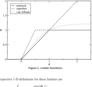
minmod superbee van Albada
Figure 1. Limiter functions.
respective 1-D definitions for these limiters are
ψ(Φ) =
min(Φ,1), max(min(2Φ,1),min(Φ,2)),
Φ2+Φ/ Φ2+1,
(31)
and the respective function plots are shown in Fig. 1. The total variation diminishing (van Leer, 1979; Barth and Jespersen, 1989) region is limited between the minmod and the superbee curves. In the previous equations,Φis defined as the ratio between the gradients of adjacent control volumes in the interface, which in a 1-D finite-difference context yields
Φ=Φi+1/2= (qi+1−qi)/(qi−qi−1). (32)
One should observe that the minmod and superbee limiters require the evaluation of maximum and minimum functions, which characterizes these limiters as nondifferentiable. The van Albada limiter, on the other hand, is continuously differentiable. This aspect is discussed further in the forthcoming paragraphs.
Limiter formulations
In a similar sense as discussed for the f ROE upwind scheme, the usual way of computing limiters is to perform such calculation every time the new numerical flux should be updated. The limiter computation work, though, is a very expensive task, amounting to more than half of an iteration computational effort, in the present context. Therefore, the idea of freezing the limiter along with the dissipation operator at some stages of the multistage time-stepping scheme seems to be very attractive in terms of possible computational resource savings. This possibility is proposed and addressed in terms of numerical solution quality and computational resource usage in the present work. Limiter computation options are now discussed in the forthcoming subsections.
Barth and Jespersen multidimensional limiter implementation (MU SCLBJ). In this method, the extrapolated property in the k-th face of the i-th cell is bounded by the maximum and minimum values over the i-th cell centroid and its neighbor cell centroids (Barth and Jespersen, 1989). This TVD interpretation can be mathematically written as
q−i ≤(qi)k≤q+i , (33)
where
q+i =max qi,qneighbors
, q−i =min qi,qneighbors
. (34)
The Barth and Jespersen (1989) limiter computation in the i-th cell is initiated by collecting the minimum, q−i , and the maximum,
q+i, values for the generic q variable in the i-th cell and its neighboring cell centroids. A limiter is computed at each j-th vertex of the control volume as
ψj(Φ) =
min 1,num+BJ/denBJ , if denBJ>0 , min 1,num−BJ/denBJ
, if denBJ<0 ,
1 , if denBJ=0 ,
(35)
where
denBJ = (qi)j−qi,
num+BJ = q+i −qi, (36)
num−BJ = q−i −qi.
The j-th vertex property is extrapolated from the i-th cell centroid with the aid of Eq. (28), such as(qi)j=qi+∇q·~rji, where~rjiis the distance vector from the i-th cell centroid to the j-th vertex. Barth and Jespersen (1989) argue that the use of the property in the cell vertices gives the best estimate of the solution gradient in the cell. The limiter value for the i-th control volume,ψi, is finally obtained as the minimum value of the limiters computed for the vertices. The control volume limiter,ψi, is eventually used to obtain the limited reconstructed property in the face, as shown in Eq. (30).
General multidimensional limiter implementation (MU SCLge). The current extension of the 1-D limiters to the multidimensional case is originally based on the work of Barth and Jespersen (1989). Moreover, Azevedo, Figueira da Silva and Strauss (2010) also present some insights into this effort in a 2-D case. The present work, however, presents a further extension of the methodology of Azevedo, Figueira da Silva and Strauss (2010). This extension is aimed at allowing the user the choice of any desired limiter formulation. Barth and Jespersen (1989) proposal is a complete limiter implementation in itself, and it has some advantages as well as disadvantages. One of such disadvantages is that it is not a continuous limiter. This aspect is discussed further in the present work. In order to allow for a general multidimensional limiter implementation, a further extension to the work of Barth and Jespersen (1989) is here proposed.
The difficulty in implementing a TVD method in a
multidimensional unstructured scheme is related to how to define the gradient ratio,Φ. The definition forΦin Eq. (32) is suitable for a finite-difference context. Nevertheless, if one considers Eq. (32) as the ratio of the central- to the upwind-difference of q, both evaluated at the interface i+1/2, and also considering the bounding definition for the property in the face in Eq. (33), then a generalization of Eq. (32) to the k-th face of the i-th cell of an unstructured grid can be obtained as
Φ= (Φi)k=
q±i −qi/|~rmi| ((qi)k−qi)/|~rki|
, (37)
where q±i is defined in Eq. (34) and the extrapolated property in the face,(qi)k, is given by
In the previous definitions,~rmiis the vector distance from the i-th cell centroid to its m-th neighbor cell centroid;~rkiis the vector distance from the i-th cell centroid to the k-th face centroid.
In this formulation, considering a quasi-uniform grid, in which
|~rmi| ≈2|~rki|, the numerator ofΦin Eq. (37) can be rewritten as 1
|~rmi|
q±i −qi ≈ 1 2|~rki|
q±i −qi=
= 1
|~rki|
q±i +qi 2 −qi
= (39)
= 1
|~rki| q±k−qi
,
where q±k are the maximum and minimum properties, in the sense of Eq. (34), though obtained at the centroid of the faces that compose the
i-th control volume. The q±k variables can be mathematically defined as
q+k =max qi,qf aces
, q−k =min qi,qf aces
, (40)
where the property in the faces, qf aces, is the arithmetic average of the properties in the neighboring cells, as in Eq. (5). The multidimensional gradient ratio for an unstructured grid face is finally obtained as
Φ=
num+/den , if den>0 ,
num−/den , if den<0 ,
1 , if den=0 ,
(41)
where
den = (qi)k−qi,
num+ = q+k −qi, (42)
num− = q−k −qi.
We now take the already presented Barth and Jespersen (1989) limiter formulation, though defined for the k-th cell face rather than the originally described cell vertex situation, and compare it with the previous generic gradient ratio definition. With the aid of Eq. (39), it can be concluded that the Barth and Jespersen limiter can be rewritten in terms of the previous generic gradient ratio as
ψk(Φ) =
min 1,2num+/den , if den>0 , min 1,2num−/den , if den<0 ,
1 , if den=0 ,
(43)
with den, num+and num−previously defined in Eq. (42). From the previous result, it can be observed that the Barth and Jespersen limiter recasts the superbee limiter in the 0≤Φ≤1 region, for a 1-D case. Similar conclusions have already been presented in the literature, as in Bruner (1996).
The advantage of the gradient ratio definition in Eqs. (41) and (42) is that it can be directly used in any other limiter definition, such as the ones presented in Eq. (31). It can also be used to recast the original Barth and Jespersen limiter formulation, as previously discussed, with a slight modification though. As also discussed, the original Barth and Jespersen limiter uses extrapolated properties in the nodes to build the gradient ratio, while extrapolated properties in the faces are preferred in the current implementation. Considering the Barth and Jespersen vertex choice in the current gradient ratio definition (Eq. (41)), it can be observed that
Φ(correct)=num±/|~rki| den/|~rji|
=|~rji| |~rki|
num±
den
=|~rji| |~rki|Φ
(implemented)
=⇒ Φ(implemented)=|~rki| |~rji|Φ
(correct). (44)
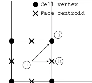
Cell vertex
Face centroid
i
k
j
Figure 2. Overview of the original and modified limiters in a 2-D application.
In this formulation, the mesh intervals |~rji| and |~rki| cannot be cancelled as in Eq. (39). Moreover, as exemplified in Fig. 2, the distance ratio, |~rki|/|~rji|, is lower than one, which results is an implemented gradient ratio that is smaller than the correct one. This difference yields smaller limiter values, which can be interpreted as an undesired increase of diffusivity in the limiter implementation. This issue can be avoided with the use of extrapolated face properties, as proposed in Eqs. (41) and (42).
Thus, the complete definition for the current multidimensional limiter is finally presented. The computation of the limiter in the i-th cell is initiated by collecting the minimum, q−k, and the maximum,
q+k, values for the generic q variable in the centroid of the faces that compose this i-th cell, according to Eq. (40). The k-th face generic property, qk, for instance, is defined as qk= (qi+qm)/2, where the m-th cell shares the k-th face with the i-th cell. For each
k-th face centroid, the property(qi)k=q(xk,yk,zk)in that centroid is extrapolated as in Eq. (38). The gradient ratio necessary to compute the limiter value is obtained through Eq. (41). A limiter is computed at each face of the control volume. The limiter value for the i-th control volume is finally obtained as i-the minimum value of i-the limiters computed for the faces.
Smooth multidimensional limiter implementation. The
nondifferentiable aspect of the minmod, superbee and Barth and Jespersen limiters poses some numerical difficulties in their utilization for practical numerical simulations. Their discontinuous formulation allows for limit cycles that hamper the convergence of upwind inviscid and viscous flow simulations to steady state (Venkatakrishnan, 1995). Furthermore, such limiters are also insensitive to the relative magnitudes of the neighboring gradients. This problem can be found in shock wave regions, where nondifferentiable limiters may present oscillations, or even in apparently smooth regions, such as farfield regions, where such limiters may respond to random machine-level noise.
Another option is to use differentiable (or continuous) limiters instead of the ones which require maximum and minimum functions. Some examples can be found in Venkatakrishnan (1995), for instance. In that work, the continuous limiters are also augmented with a control parameter to drive the smoothness of the limiter in small-amplitude oscillation regions, and also to allow for a smooth transition from limiting to nonlimiting state. In that formulation (Venkatakrishnan, 1995), this limiter control is made grid-dependent in order to sensitize the local gradients to the local grid size, therefore eliminating small extrema oscillations. Although such control actually allows for machine-zero convergence, it seems that it somehow poses a trade-off between convergence and obtaining monotone (oscillation-free) steady-state solutions.
The option chosen in the present work is to remove the grid dependence of the limiter control and to add, instead, a constant threshold value. The van Albada limiter, rewritten for such modification, is given by
ψ num±,den=num
± num±+den+ǫLIM
num±2+
den2+ǫLIM , (45)
whereǫLIM is the constant limiter control, chosen asǫLIM=10−4 in the present work. This option seems to be appropriate for all aerospace cases considered by the present and other development groups (see, for instance, Oliveira, 1999), always allowing machine-zero steady-state convergence for monotone numerical solutions. These aspects are further analyzed in the results of the present work.
Results and Discussion
The flux computation schemes presented in the previous sections are applied to inviscid and viscous flows about typical aerospace configurations. Firstly and foremost, the actual order of accuracy of the discretization scheme is assessed. The influence of the numerical schemes on shock-wave resolution is, then, addressed with a 1-D shock-tube problem, and a transonic inviscid flow about a typical supercritical airfoil. Boundary layer flows are also addressed, for subsonic laminar flows about a flat plate configuration, with Reynolds number Re=105and Mach number M
∞=0.254.
Discretization order of accuracy
The current method for assessing the discretization order of accuracy is based on the verification methodology presented by Roache (1998) and the discretization order of accuracy estimation procedure from Baker (2005). In the current methodology, a source term carrying information of a generically prescribed solution for the RANS equations is explicitly added to the RHS operator in order to drive the numerical solution to the prescribed one (Roache, 1998). The difference between the converged computational solution and the original one is taken as a measure of the accuracy of the method, as well as a confirmation of the correctness of the implementation (Baker, 2005; Bigarella, 2002).
For this verification effort, the chosen physical domain is a hexagonal block with unit sides. Several grid configurations are used for the simulations, including different number of grid points and different control volume types. The following sets of grids are used:
1. Uniformly spaced hexahedral meshes with 25×25×25, 50×
50×50 and 75×75×75 points;
2. Two isotropic tetrahedral meshes with 25×25×25 and 50×
50×50 control points in the domain edges.
With the chosen computational meshes, the authors attempt to address the behavior of the numerical code with grid characteristics such as refinement and topology. This evaluation is performed for the four flux schemes available in the current code, namely the MAVR, MATD, CUSP and f ROE schemes. For the CUSP and f ROE schemes, the van Albada limiter is chosen.
In this work, 2nd-order-accurate approximations for convective flux computations are available. Hence, the numerical error of the method as function of the mesh spacing can be written as
error∝ ∆x2, (46)
where∆x, in the current study, is taken as the arithmetic average of
the cubic root of the cell volumes, for each of the previously described grids. If one takes the logarithm of both sides of Eq. (46), that equation can be rewritten as
log (error)∝2 log(∆x). (47)
The logarithm of the theoretical error of the method has a slope of two when plotted against the logarithm of the grid spacing. The actual spatial accuracy of the method, however, may be different from that presented in Eq. (47). The actual error can be written for a general case as
log (error)∝αlog(∆x), (48)
whereα is the slope of the actual spatial accuracy curve that is attained with the implemented scheme. The error is here taken as the RMS value of the difference between the prescribed and numerical density fields.
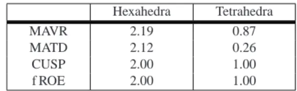
Table 1. Error slopes for different mesh and flux scheme settings.
Hexahedra Tetrahedra
MAVR 2.19 0.87
MATD 2.12 0.26
CUSP 2.00 1.00
f ROE 2.00 1.00
The resulting slopes are collected in Table 1. From these results, it can be observed that all flux schemes sustain the nominal 2nd-order accuracy for the uniformly-spaced hexahedral meshes. The order of accuracy deteriorates for the tetrahedral meshes. The switched artificial dissipation schemes (MAVR and MATD) present larger accuracy losses than the MUSCL-reconstructed counterparts (CUSP and f ROE). The latter schemes present less mesh topology dependency, which is an indication of increased robustness that one would like to have under highly-demanding or even inadequate mesh cells.
In Mavriplis (1997), it is argued that routine upwind schemes, such as the ones here used, are commonly applied in “a quasi-one-dimensional fashion normal to control-volume faces”. Although the reconstruction and limiter formulations used in the paper are truly multidimensional, the background upwind flux schemes are not, and they “may misinterpret flow features not aligned with control volume interfaces” (Mavriplis, 1997). The current authors attribute the observed loss of accuracy in the tetrahedral grid cases analyzed before to this misalignment behavior.
by Mavriplis (1997), Deconinck, Roe and Struijs (1993), Sidilkover (1994), Peroomian and Chakravarthy (1997), Deconinck and Degrez (1999), Jawahar and Kamath (2000), and Drikakis (2003). These references, in particular, present efforts towards the development of numerical schemes that are less sensitive to mesh topology, and that present native multidimensional “cell-transparent” behavior. This is certainly an interesting development to be brought to the current code context, but it is beyond the scope of the present work.
1-D shock tube
Computations of 1-D shock-tube inviscid flow cases are considered. Numerical results are compared to the analytical solution for this problem. For the numerical simulations, an equivalent 3-D grid composed of a line of 500 hexahedra is used. The initial dimensionless density condition for the left half part of the shock tube isρLini=1, whereas on the right half,ρRini=20. The reference conditions are taken in the initial state of the low pressure side of the shock tube. Equal temperatures are assumed at both sides of the shock tube. Several other simulations with different density ratios have also been performed and the results are essentially similar to the ones presented in the forthcoming analyses. A constant dimensionless time step of∆t=10−5 is used for this transient solution, and the forthcoming plots are taken at t=0.1.
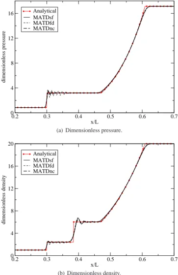
MATD results. The three possible implementation forms of the MATD artificial dissipation method are here assessed. The MAT Ds f option is the straightforward extension of the nominal finite-volume scalar artificial dissipation (MAVR) to a matrix version. The advantageous implementation form as found in a finite-difference context cannot be used due to the necessity of performing a surface integral of the scaling matrix. Another option, namely MAT Df d, uses this attractive finite-difference-like implementation form, which unfortunately is not in accordance with the current finite volume artificial dissipation framework formulation. This option is only considered here to verify this previous assertive. Finally, a mixed version that allows for a surface-integrated scaling matrix, though in a nonconservative form, with the same advantageous finite-difference-like matrix implementation, here termed MAT Dnc, is suggested.
Dimensionless pressure and density distributions along the tube longitudinal axis are presented in Fig. 3. One can clearly observe in this figure that all MATD options allow for pre- and post-discontinuity oscillation to build up. The less correct MAT Df d option presents much larger oscillations, whereas the MAT Dnc option presents the lowest levels of oscillation. All options, however, correctly follow the analytical result trends. In terms of computational resource usage, the finite-difference-like implementation does present advantages over the finite volume form. The MAT Df dand MAT Dncoptions require about 30% less computational time than the MAT Ds fformulation for this test case.
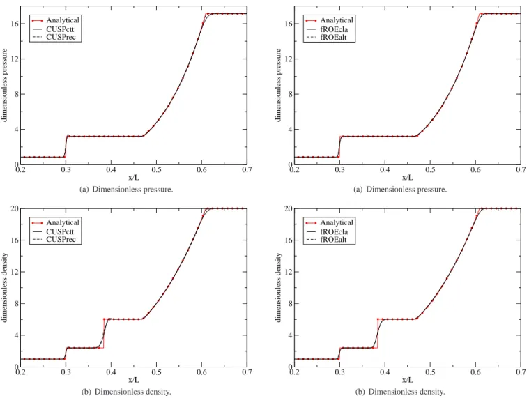
CUSP results. The CUSP scheme implementation options are here addressed. The CU SPctt formulation (Jameson, 1995a; Jameson, 1995b; Swanson, Radespiel and Turkel, 1998) uses constant property distributions in the cell to build the centered convective fluxes, whereas the CU SPrec option proposed in the current work uses reconstructed properties in the faces to compute such fluxes. The dissipation formulation is identical between both options, and a value ofǫCU SP=0.3 is chosen for the CUSP constant. The van Albada limiter is used here in the reconstruction process within the proposed
0.2 0.3 0.4 0.5 0.6 0.7 x/L
0 4 8 12 16
dimensionless pressure
Analytical MATDsf MATDfd MATDnc
(a) Dimensionless pressure.
0.2 0.3 0.4 0.5 0.6 0.7 x/L
0 4 8 12 16 20
dimensionless density
Analytical MATDsf MATDfd MATDnc
(b) Dimensionless density.
Figure 3. Property distributions along the shock tube obtained with different MATD model options.
multidimensional limiter implementation. The limiter computation is only performed in alternate stages of the Runge-Kutta time step.
Swanson, Radespiel and Turkel (1998) argue that the original CUSP scheme formulation, here termed CU SPctt, does not nominally provide oscillation-free shocked-flow results. The current authors believe this behavior is due to the computational form of the centered convective fluxes, which uses constant properties in the cells in the original formulation. The authors believe that the use of reconstructed properties in the faces to build such fluxes may overcome such limitation. These arguments are corroborated by the pressure and density results presented in Fig. 4. Both CUSP implementation options compare very well with the analytical solution. It can be observed in Fig. 4 that the original CU SPcttformulation does allow oscillations to build up near discontinuities, while the proposed
CU SPrec option prevents such undesired behavior. Furthermore, the latter option also exhibits a crisper representation of the high-pressure-side expansion region. Finally, the CU SPrecimplementation requires less than 10% additional computational time than the original formulation to compute the current test case.
0.2 0.3 0.4 0.5 0.6 0.7 x/L
0 4 8 12 16
dimensionless pressure
Analytical CUSPctt CUSPrec
(a) Dimensionless pressure.
0.2 0.3 0.4 0.5 0.6 0.7 x/L
0 4 8 12 16 20
dimensionless density
Analytical CUSPctt CUSPrec
(b) Dimensionless density.
Figure 4. Property distributions along the shock tube obtained with different CUSP scheme options.
convective flux plus upwind artificial dissipation terms computed in alternate stages of the Runge-Kutta time marching procedure. Limiter settings are exactly the same as used for the previous CUSP scheme simulations. Pressure and density distributions for the Roe scheme are presented in Fig. 5. Numerical solutions compare very well with the analytical one, and no oscillation near discontinuities can be found in the numerical solution. It is interesting to observe that no differences between f ROEclaand f ROEalt options can be observed. The f ROEcla scheme, however, is about twice as expensive as the
f ROEaltimplementation, proposed in the present paper.
MUSCL results. The original Barth and Jespersen multidimensional limiter (MU SCLBJ) is compared to the generic multidimensional implementation (MU SCLge)proposed in the work. The minmod, van Albada and superbee limiters are considered in order to demonstrate the capability of the current multidimensional reconstruction scheme to handle various limiter types. For this study, the f ROEaltscheme is used with limiter computations at alternate stages of the Runge-Kutta scheme. Pressure and density results for the previous limiter options are shown in Fig. 6. One can clearly observe in this figure that the correct solution is obtained for all cases, which demonstrates that the current multidimensional reconstruction scheme does allow for the use of various limiter formulations. In general, no oscillatory behavior
0.2 0.3 0.4 0.5 0.6 0.7 x/L
0 4 8 12 16
dimensionless pressure
Analytical fROEcla fROEalt
(a) Dimensionless pressure.
0.2 0.3 0.4 0.5 0.6 0.7 x/L
0 4 8 12 16 20
dimensionless density
Analytical fROEcla fROEalt
(b) Dimensionless density.
Figure 5. Property distributions along the shock tube obtained with different f ROE scheme options.
in the numerical solutions can be observed in the results, regardless of the limiter formulation used. The comparison with the analytical solution is also very good, with the superbee limiter presenting crisper discontinuities, as expected, due to its less diffusive formulation. As already discussed, the Barth and Jespersen limiter recasts the superbee limiter in the 0≤Φ≤1 range, in the 1-D case. This is confirmed in Fig. 6, since the former limiter results are virtually identical to the latter ones. The van Albada limiter results lie within the more-and the less-diffusive minmod more-and superbee limiters, respectively, as expected. It should be remarked here that its augmented smoothness cannot be demonstrated in this transient case since it is a feature designed for steady problems.
2-D supercritical airfoil
0.2 0.3 0.4 0.5 0.6 0.7 x/L
0 4 8 12 16
dimensionless pressure
Analytical BJ Minmod van Albada Superbee
(a) Dimensionless pressure.
0.2 0.3 0.4 0.5 0.6 0.7 x/L
0 4 8 12 16 20
dimensionless density
Analytical Barth and Jespersen Minmod
van Albada Superbee
(b) Dimensionless density.
Figure 6. Property distributions along the shock tube obtained with different limiter implementation options.
and the angle of attack isα=1.4 deg. In the present simulations, three grid levels in a “V” cycle, with one iteration before and after property restrictions and prolongations, are used in the multigrid method. The
CFL number in all flux computation schemes is set to CFL=1.25. The numerical schemes are evaluated at a multidimensional shocked flow in order to assess their capability at correctly solving such test cases. Moreover, numerical results are not compared to experimental ones in this case because viscous terms and turbulence modeling are not included in the present calculations.
MATD results. The three possible implementation forms of the MATD artificial dissipation method, namely MAT Ds f, MAT Df dand MAT Dnc, are here assessed. Pressure coefficient distributions and the residue histories are presented in Fig. 7. It can be observed in Fig. 7(a) that the three C p distributions present differences. The MAT Ds f results seem to present a larger amount of dissipation. The MAT Df d option presents several oscillations near the shock wave discontinuity. This observation corroborates the assertive that the present switched artificial dissipation model is calibrated to receive only surface-integrated coefficients, which is not the case for the MAT Df doption. The MAT Dnc formulation avoids such oscillation problem while allowing less dissipative results at lower costs, i.e., approximately 30% cheaper than the MAT Ds f option. Residue histories show that
0 0.25 0.5 0.75 1 x/c
-1 -0.5 0 0.5 1
-Cp
MATDsf MATDfd MATDnc
(a) C p distributions.
0 1000 2000 3000 cycles
-8 -6 -4 -2 0
log RHSmax
MATDsf MATDfd MATDnc
(b) Density residue histories.
Figure 7. Simulation results for the supercritical airfoil obtained with different MATD model options.
both options, which include some surface integration in the definition of the scaling terms of the artificial dissipation, namely MAT Ds fand MAT Dnc, converge well for this case, while the MAT Df dformulation presents convergence stall due to the oscillatory behavior of the solution.
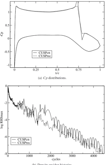
CUSP results. The CU SPcttand CU SPrecscheme options are here addressed. Numerical settings are taken similarly to the previous 1-D shock tube case. C p distributions and residue histories for these cases are presented in Fig. 8. As already observed in the 1-D case, the original CU SPctt implementation allows for oscillations to build up in the solution. This undesired behavior is avoided with the use of reconstructed properties in the faces to compute the convective flux terms. The convergence of the CU SPrec option seems to be more robust than the CU SPctt implementation, mainly because of the lack of oscillatory structures in the numerical solution.
0 0.25 0.5 0.75 1 x/c
-1 -0.5 0 0.5 1
-Cp
CUSPctt CUSPrec
(a) C p distributions.
0 1000 2000 3000 4000 cycles
-8 -6 -4 -2 0
log RHSmax
CUSPctt CUSPrec
(b) Density residue histories.
Figure 8. Simulation results for the supercritical airfoil obtained with different CUSP model options.
differences can be observed between the two solutions, in terms of both numerical resolution of the flow properties, i.e., airfoil pressure coefficient in this particular case, and residue histories, as shown in Fig. 9. The f ROEalt option, however, converges in almost half the computational time used by the classical f ROEcla implementation. The reader should observe that Fig. 9(b) is showing the residue histories as a function of multigrid cycles. However, the f ROEalt option costs almost half the computational time of the f ROEcla option per multigrid cycle. These results, once again, show that the same quality of numerical solution and convergence rate can be obtained with the proposed implementation method at much lower computational resource usage.
MUSCL results. The original Barth and Jespersen multidimensional limiter (MU SCLBJ) is compared to the here proposed generic multidimensional implementation (MU SCLge). The minmod, van Albada and superbee limiters are considered within the generic multidimensional reconstruction scheme. Numerical settings similar to those used in the 1-D shock tube case are also considered for the present study. C p distributions and residue histories for these cases are presented in Fig. 10. No oscillatory behavior in the numerical solutions can be observed in all presented results. The solutions
0 0.25 0.5 0.75 1 x/c
-1 -0.5 0 0.5 1
-Cp
fROEcla fROEalt
(a) C p distributions.
0 1000 2000 3000 cycles
-8 -6 -4 -2 0
log RHSmax
CUSPctt CUSPrec
(b) Density residue histories.
Figure 9. Simulation results for the supercritical airfoil obtained with different f ROE scheme options.
with the superbee and the Barth and Jespersen limiters present crisper discontinuities, as already observed in the shock-tube case. As also already observed, the van Albada limiter results lie within those of the minmod and superbee limiters.
It is interesting to observe in the residue histories in Fig. 10(b) that the minmod, Barth and Jespersen and superbee limiters present residue stall. As already discussed, this behavior is due to their discontinuous formulation, which involves the evaluation of maximum and minimum functions. The continuous van Albada option, on the contrary, allows for automatic residue convergence, that is, convergence without the need for user inputs such as limiter freezing.
0 0.25 0.5 0.75 1 x/c
-1 -0.5 0 0.5 1
-Cp
Barth and Jespersen Minmod
van Albada Superbee
(a) C p distributions.
0 1000 2000 3000 cycles
-8 -6 -4 -2 0
log RHSmax
Barth and Jespersen Minmod
van Albada Superbee
(b) Density residue histories.
Figure 10. Simulation results for the supercritical airfoil obtained with different limiter implementations.
the previously discussed flux computation schemes, are presented in Fig. 11(b) for the 255×64-cell computational grid. One can observe in this figure that all numerical schemes yield results that are very similar to each other at computing a crisp shock-wave discontinuity and overall pressure distributions. These computational results can, therefore, be considered as a reasonable reference solution for further comparisons in the paper.
It should also be remarked here that the numerical results are not compared to experimental results because an inviscid approximation is considered for the numerical simulations, which is not representative of the actual turbulent viscous wind-tunnel flow. The main interest here is the behavior of the numerical schemes at computing shocked flows at successively refined computational grids. Pressure coefficient distributions over the profile obtained with different meshes and flux computation schemes are presented in Fig. 12. In this figure, one can observe that the MAVR scheme presents considerable variations in the results as the grid is refined. Moreover, the shock wave position also varies considerably with grid refinement. More consistent results can be obtained with the MATD model. Differences among the solutions are much smaller in this case and the shock wave position presents less changes with grid refinement. The CUSP and f ROE schemes present even more consistent results, and the variations in the numerical solution with grid refinement are
(a) Computational grid.
0 0.25 0.5 0.75 1 x/c
-1 0 1
-Cp
MAVR MATD CUSP fROE
(b) C p distributions.
Figure 11. 2-D view of the grid over the supercritical airfoil with255×64
cells, and respective wall C p distributions obtained with different flux computation schemes.
much less pronounced in these cases. The numerical results obtained with both models are comparatively much similar to each other, with the CUSP scheme presenting slightly better results.
Subsonic flat plate
0 0.25 0.5 0.75 1 x/c
-1 0 1
-Cp
100 x 24 grid 150 x 40 grid 255 x 64 grid
(a) MAVR model.
0 0.25 0.5 0.75 1
x/c -1
0 1
-Cp
100 x 24 grid 150 x 40 grid 255 x 64 grid
(b) MATDncmodel.
0 0.25 0.5 0.75 1
x/c -1
0 1
-Cp
100 x 24 grid 150 x 40 grid 255 x 64 grid
(c) CUSPrecmodel.
0 0.25 0.5 0.75 1
x/c -1
0 1
-Cp
100 x 24 grid 150 x 40 grid 255 x 64 grid
(d) f ROEaltscheme.
Figure 12. WallC pdistributions over the supercritical airfoil obtained with different flux computation schemes and computational grids.
-2 -1.5 -1 -0.5 0 0.5 1
0 0.5 1
(a) Full view.
0.6 0.65 0.7 0.75
0
(b) Detail.
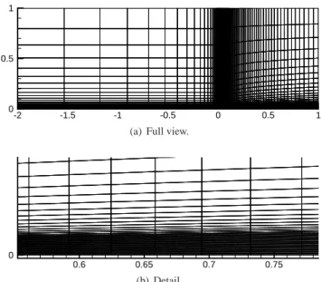
Figure 13. 2-D views of the grid over a flat plate with 20 points inside the boundary layer.
The corresponding mesh generator places a user-provided number of computational cells inside the boundary layer. These cells are evenly spaced along the wall-normal direction, and they extend to a user-defined height,ηmax, given by a Blasius-transformed length, which is defined asη= (y/x)√Rex. Therefore, the physical height of the boundary layer points varies with the longitudinal position, following the theoretical growth of the boundary layer up to the value ofηmax. This grid construction allows the user to keep a constant number of points inside the boundary layer along the flat plate length. In the actual implementation, however, in order to avoid numerical difficulties near the plate leading edge, this assertive is valid for the last three quarters of the flat plate length. This specific grid construction requires the knowledge of the flow Reynolds number, which should be correctly provided by the user. The plate length is fixed as one and the grid extends two lengths upstream of the plate leading edge, and one length along the normal direction. Outside the boundary layer, an automatic exponential growth guarantees the normal direction length extension and a sufficiently low number of control volumes. One quarter of the number of points specified by the user for the longitudinal direction is placed in the two-length space ahead of the plate, and the remaining points are placed along the plate longitudinal direction. These points are clustered near the flat plate leading edge in order to account for the larger gradients that are expected in this region.
0 0.25 0.5 0.75 1 u/Uinf
0 2 4 6 8 10
η
10 points 20 points 40 points Blasius
(a) MAVR model.
0 0.25 0.5 0.75 1
u/Uinf 0
2 4 6 8 10
η
10 points 20 points 40 points Blasius
(b) MATDncmodel.
0 0.25 0.5 0.75 1
u/Uinf 0
2 4 6 8 10
η
10 points 20 points 40 points Blasius
(c) CUSPrecmodel.
0 0.25 0.5 0.75 1
u/Uinf 0
2 4 6 8 10
η
10 points 20 points 40 points Blasius
(d) f ROEaltscheme.
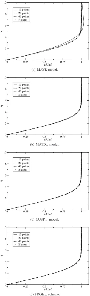
Figure 14. Laminar boundary layer profiles over a flat plate obtained with different flux computation schemes and computational grids.
is interesting to observe that the upwind f ROE scheme, as well as the centered MATD and CUSP models, guarantee the correct solution with all tested grid configurations. The MAVR centered scheme presents an anomaly in the bend of the boundary layer profile for the grids with a smaller number of points in the boundary layer, as also verified by Bigarella, Moreira and Azevedo (2004). The oscillation, nevertheless, decreases with the increasing number of points inside the boundary layer. It is only with the 40-point grid configuration that the correct solution can be obtained with the MAVR model.
Concluding Remarks
The paper presents results obtained with a finite volume code developed to solve the RANS equations over aerospace configurations. Several flux computation schemes are considered in the paper. The convective fluxes can be computed by either a centered scheme plus explicitly added artificial dissipation terms, or the Roe upwind scheme. For the centered scheme, three artificial dissipation models are addressed, namely a scalar and a matrix version of a switched model, and the CUSP scheme.
Multidimensional interpolation is used in order to achieve second-order accuracy for schemes that require property reconstruction. An extension to the work of Barth and Jespersen is proposed and evaluated in the paper. Such extension aims at decreasing the level of dissipation added by the original limiter formulation, which has been verified in the presented results. As a byproduct of such effort, various limiter formulations can also be used within the multidimensional unstructured code structure. A smooth limiter option is also proposed and used to achieve machine-zero convergence of monotone numerical solutions without user interference.
Several formulation and implementation approaches for such methods are proposed and assessed in the paper in order to enhance robustness, numerical accuracy and computational efficiency of the numerical tool for aerospace flow cases. Comparisons of numerical boundary layers for a zero-pressure gradient flat plate laminar flow with the corresponding theoretical Blasius solution show the level of accuracy that can be obtained with the present formulation. It is observed that the scalar artificial dissipation model presents a very large dependency on the grid density. For this model, about 40 cells inside the boundary layer are required to correctly solve the boundary layer flow. The matrix artificial dissipation model, as well as the CUSP and the Roe schemes, require only 10 points to achieve the same level of accuracy. The grid-independent converged solutions, for all methods, are very close to the theoretical Blasius solution.
The code is also able to correctly solve for more complex flows, such as the transonic flow about a typical supercritical airfoil. The ability of the flux computation schemes in calculating shock waves in the solution is assessed in the present study, in particular with regard to the dependency with grid density. It is observed that more consistent solutions can be obtained with the Roe and CUSP schemes, to which small variations with grid refinement are verified. The scalar artificial dissipation model is not so effective in these analyses, and a considerable dependency of the numerical solution with the grid configuration is observed. The matrix version of the switched artificial dissipation model presents more consistent results than its scalar counterpart.