European integration and banking efficiency: a panel cost frontier approach

(1)

Carlos Pestana Barros & Nicolas Peypoch

A Comparative Analysis of Productivity Change in Italian and Portuguese Airports

WP 006/2007/DE _________________________________________________________

Cândida Ferreira

European integration and banking efficiency: a panel cost

frontier approach

WP 03/2011/DE/UECE _________________________________________________________

Department of Economics

W

ORKING

P

APERS

ISSN Nº 0874-4548

School of Economics and Management

(2)

1

European integration and banking efficiency: a panel cost frontier approach

Cândida Ferreira[1]

Abstract

The aim of this paper is to contribute to the relatively scarce published research on the

relationship between European integration and banking efficiency. Estimating cost translog

frontier functions for different panels of European Union countries for the time period

1994-2008 we conclude that there is always technical inefficiency. Additionally, although country

inefficiencies have decreased in recent years (2000-2008), there are no remarkable changes in

the countries’ ranking positions. Our results also point to the existence of a quite slow

convergence process across EU countries during the period analysed, as well as its acceleration

after the establishment of the European Monetary Union.

Keywords: Bank efficiency; European integration; convergence; cost frontier approach.

JEL Classification: G15; G21; F36; C58.

[1]

ISEG-UTL - Instituto Superior de Economia e Gestão – Technical University of Lisbon

and UECE – Research Unit on Complexity and Economics

Rua Miguel Lupi, 20, 1249-078 - LISBOA, PORTUGAL tel: +351 21 392 58 00

(3)

2

European integration and banking efficiency: a panel cost frontier approach

1. Introduction

In recent years, financial systems have been experiencing the consequences of the strong

imbalances and turbulence of the US sub-prime mortgage market, which affected different

segments of the international money and credit markets and revealed the fragility of many

financial institutions.

The ensuing crisis has raised attention to the importance of studies aiming to identify the factors

explaining the weaknesses in the financial systems at national and international levels. It has

also intensified the questioning of the role of the financial authorities and their policy responses

in order to detect the symptoms of fragility and prevent further crisis and instability.

It remains true that the European Union (EU) financial and credit systems are bank-dominated

and among EU regulators, there is a strong belief that a well-integrated financial system is a

necessary precondition for the enhancement of financial stability and the increased efficiency of

the entire EU economy.

Moreover, the process of financial integration is often presented as a necessary pre-requisite for

the adoption of the euro and the implementation of the single monetary policy, with the

predominance of the banking intermediation in the context of the EU (Cabral et al., 2002;

European Central Bank, 2003; Hartmann et al., 2003; Baele et al., 2004; Sørensen and

Gutiérrez, 2006; Arghyrou et al., 2009).

The establishment of the European Monetary Union was supposed to accelerate the process of

consolidation and economic and financial integration. However, there is no clear consensus on

(4)

3

empirical studies conclude that there is evidence of integration, particularly of the European

money market, but also to some extent of the bond and equity markets (Cabral et al. 2002;

Hartmann et al., 2003; Guiso et al., 2004; Manna, 2004; Cappiello et al., 2006; Bos and

Schmiedel, 2007). Other empirical contributions have concluded that the European financial

markets are far from being integrated (Gardener et al., 2002; Schure et al. 2004; Dermine, 2006;

European Central Bank, 2007; European Central Bank, 2008; Affinito and Farabullini, 2009;

Gropp and Kashyap, 2010).

The European banking institutions play a unique role, first in the context of the Single Market

Program and then of the European Monetary Union, as the increase of competition in all

financial-product market segments was expected to contribute to price and cost reductions and

benefit the exploitation of scale economies.

There is a large strand of literature on the analysis of the determinants of efficiency and

particularly on the empirical measurement of the profit and cost efficiency in banking (among

others, Altunbas et al., 2001; Goddard et al. 2001, 2007; Williams and Nguyen, 2005; Kasman

and Yildirim, 2006; Barros et al. 2007; Berger, 2007; Hughes and Mester, 2008; Sturm and

Williams, 2010).

Nonetheless, few studies have clearly addressed the relationship between European integration

and banking efficiency. The main examples are to be found in Tortosa-Ausina (2002), Murinde

et al., (2004), Holló and Nagy (2006), Weill (2004, 2009) and Casu and Girardone (2009,

2010).

This paper tests banking efficiency across European Union countries in the wake of the recent

crisis, estimating translog cost frontier functions and comparing the results for different samples

of EU countries: all European Union members (EU-27), the “old” members (EU-15) and those

(5)

4

years after the introduction of the single currency (2000-2008). The conclusions point to the

existence of statistically relevant technical inefficiencies, although these have tended to decrease

during the last decade. Furthermore, the analysis of the convergence process with the estimation

of β-convergence models allows us to conclude that there is clear convergence in banking

efficiency across EU countries and that the pace of convergence increased slightly after the

implementation of the EMU.

The paper is structured as follows: Section 2 presents the theoretical framework and a brief

literature review; the methodology and the data are presented in Section 3; Section 4 reports the

obtained results; Section 5 discusses these results and concludes.

2. Theoretical framework and brief literature review

Over recent years, the research into the role and performance of the banking industry has paid

particular attention to the estimation of bank efficiency, explaining the variations in efficiencies

across banks and countries. Although European research on bank efficiency has not yet matched

the record of the US contributions, it has increased enormously since the dynamic changes were

introduced into the structure of European banking.

There is a strand of literature that focuses on the heterogeneities across banks, explaining them

by the differences in the performance conditions, such as bank size (Altunbas et al., 2001;

Molyneux, 2003; Bikker et al., 2006; Schaeck and Cihak, 2007), bank ownership (Bonin et al.,

2005; Kasman and Yildirim, 2006; Lensink et al., 2008), bank mergers (Diaz et al., 2004;

Campa and Hernando, 2006; Altunbas and Marquês, 2008), technological progress (Wheelock

(6)

5

2001; Vives, 2001; Goddard et al., 2007) and legal tradition (Berger et al., 2001; Beck et al.,

2003-a; 2003-b;Barros et al., 2007).

The analysis of bank cost efficiency is based on the assumption that the performance of each

individual bank can be described by a production function that links banking outputs to the

necessary banking inputs. However, there is no consensus concerning the definition of the

banking outputs. The discussion is mainly on the specific role of deposits, since they may be

considered both as inputs and outputs of the production function.

According to the production approach, banks provide services related to loans and deposits and,

like other producers of goods or services, they use labour and capital as inputs of a given

production function (see inter alia, Berger and Humphrey, 1991; Resti, 1997; Rossi et al. 2005).

The intermediation approach considers that banks are mainly intermediaries between the

economic agents with excess financing capacity and those economic agents that need financial

support for their investments. Banks attract deposits and other funds and, using labour and other

types of inputs such as buildings, equipment, or technology, they transform these funds into

loans and investment securities. This approach has been used, for instance, by Sealey and

Lindley (1977), Berger and Mester (1997), Altunbas et al. (2001), Bos and Kool (2006) and

Barros et al. (2007).

The research into efficiency, either by the production approach or by the intermediation

approach, is based on the estimation of an efficiency frontier with the best combinations of the

different inputs and outputs of the production process and then on the analysis of the deviation

from the frontier that corresponds to the losses of efficiency.

Most of the empirical studies on the measurement of bank efficiencies adopt either

non-parametric methods, particularly the Data Envelopment Analysis (DEA), or non-parametric methods,

(7)

6

optimisation (maximisation of profits or minimisation of costs), given the assumption of a

stochastic optimal frontier.

Following the pioneering contribution of Farrel (1957), the SFA has been developed by such

authors as Aigner et al. (1977), Meeusen and van den Broeck (1977), Stevenson (1980), Battese

and Coelli (1988, 1992, 1995), Frerier and Lowell (1990), Kumbhakar and Lovell (2000),

Altunbas et al. (2001) and Coelli et al. (2005).

According to Altunbas et al. (2001), the single equation stochastic cost function model can be

represented by the following expression: TC=TC(Q_i,P_j)+ε, where TC is the total cost, Q is

the vector of outputs, P is the input-price vector and ε is the error (a formal presentation of the

cost function for panel data models is to be found in Appendix I).

The error of this cost function can be decomposed intoε =u+v, where u and v are

independently distributed. The first part of this sum, u, is assumed to be a positive disturbance,

capturing the effects of the inefficiency or the weaknesses in the managerial performance, and is

distributed as half-normal and is truncated at zero,

[

u~Ν+

(

µ,σ_u2

)

]

, with non-zero µ mean, as

each unit´s production must lie on or below its production frontier but above zero. The second

part of the error, v, is assumed to be distributed as two-sided normal, with zero mean and

variance σ_v2 and it represents the random disturbances.

As the estimation of the presented cost function provides only the value of the error term, ε, the

value of inefficient term, u, must be obtained indirectly. Following Jondrow et al. (1982) and

Greene (1990, 2003, 2008) the total variance can be expressed as σ2 =σ_u2+σ_v2, where the

contribution of the inefficient term is ₂ 2 2 2

1 λ λ σ σ

+ =

u ; ₂

2 2

1 λ σ σ

+ =

v is the contribution of the noise

and

v u

σ σ

(8)

7

The variance ratio parameter γ, which relates the variability of u to total variabilityσ2, can be

formulated as

2 2

1 λ λ γ

+

= or

2 2

2

v u

u

σ σ

σ γ

+

= ; 0 ≤ γ ≤ 1. If γ is close to zero, the differences in the

cost will be entirely related to statistical noise, while a γ close to one reveals the presence of

technical inefficiency.

The theoretical background to financial integration can be found in the large strand of literature

that analyses price convergence, particularly in the different versions of the Law of One Price.

The Law of One Price simply states that “identical goods must have identical prices”. It is a

fundamental and intuitive proposition and it is usually considered as one of the most basic laws

in economics (Lamont and Thaler, 2003). This law is based on the assumption that price

differences would provide an opportunity for arbitrage and, in the absence of transaction costs,

the arbitrageurs would lead to price convergence.

Some authors (e.g. Baele et al., 2004; European Central Bank, 2007, 2008; Casu and Girardone,

2009, 2010) consider that full integration in the financial markets means that all potential agents

in these markets, facing a single set of financial instruments and/or services, follow a single set

of decision rules, have equal access to these financial instruments and/or services and are treated

equally when acting in these markets.

This concept of financial integration, which is closely related to the Law of One Price, supposes

that financial integration is independent of the financial structures within countries or regions.

Several works have discussed and empirically tested the validity of this law, recognising the

existence of some caveats, since markets may be incomplete, in which case financial integration

will not benefit all agents acting in these markets (e.g. Allen and Gale, 1997; Baele et al., 2004).

For different euro-area countries, Hartmann et al. (2003) find that there is no support for the

(9)

8

(2004) consider five key euro-area markets (money, government bonds, corporate bonds,

banking/credit and equity markets) and conclude that these distinct market sectors have attained

different levels of integration. Casu and Girardone (2009, 2010) also state that despite the

regulatory emphasis, the process of integration of the EU financial services sector has been

slower than in other sectors and there still remain real obstacles to the integration.

Borrowing the concepts σ-convergence and β-convergence from the economic growth theory

and the contributions of authors like Barro and Sala-i-Martin (1992), Quah (1996) or,

specifically for panel data, Weill (2009), a β-convergence test to access the speed of integration

can be performed through the estimation of the following linear equation:

∑

= − − = + + + − n i t i i t i t i t

i BPerf BPerf D

BPerf 1 , 1 , 1 ,

, ln ln

ln α β ε

Where: BPerfi,t= bank performance in country i (i = 1, ...n) in year t (t = 1, ... T) Di = country dummies

ε = error term

A negative value of the parameter β implies convergence, and this convergence will be as fast

as β is high.

3. Methodology and data used

In this paper, we follow the intermediation approach and we specify a linear cost function with

three outputs (loans, securities and other earning assets) and the price of three inputs (borrowed

funds, physical capital and labour).

The general translog form of the cost function to be estimated is:

(10)

9

Where:

C = total cost (i = 1,..., N = number of the countries included in each panel; t = 1,...,T = time period)

y = outputs (r,s = 1, ..., R) w = inputs (h,k = 1, ..., H)

z = other explaining variables (m = 1, ..., M) t = time trend

Our data are sourced from the BankScope database. The sample comprises annual data from

consolidated accounts of the commercial and saving banks of all EU countries between 1994

and 2008. In Appendix II, we present the number of banks of each country in 1994, 2000 and

2008 and also the average number of the entire period (1994-2008).

We define the input prices and the outputs (quantities) of the cost function and we use the

following variables:

• Dependent variable = Total cost (TC) = natural logarithm of the sum of the

interest expenses plus the total operating expenses

• Outputs:

o_Y₁_{= Total loans}_{= natural logarithm of the loans}

o Y2 = Total securities = natural logarithm of the total securities

o_Y₃_{= Other earning assets} ₌_{natural logarithm of the difference between the}

total earning assets and the total loans

• Inputs:

o_W₁_{= Price of borrowed funds}_{= natural logarithm of the ratio interest}

expenses over the sum of deposits

o_W₂_{= Price of physical capital}_{= natural logarithm of the ratio non-interest}

expenses over fixed assets

o_W₃_{= Price of labour}_{= natural logarithm of the ratio personnel expenses over}

the number of employees

• Other variables:

o_Z₁_{= Number of banks =}_{natural logarithm of the number of banks included in}

the panels

o Z2 = Equity ratio = natural logarithm of the ratio equity over total assets

o_Z₃_{= Ratio revenue over expenses =}_{natural logarithm of the ratio of the total}

revenue over the total expenses

o_{t = Time trend}

In our estimations we consider three sets of EU countries:

• EU-27 – all EU member-states.

(11)

10

• EU-15 – comprising the 15 “old” EU member-states: Austria, Belgium,

Denmark, Finland, France, Germany, Greece, Ireland, Italy, Luxembourg, Netherlands, Portugal, Spain, Sweden and UK.

• EU-12 – comprising the 12 member-states that have joined the union since

2004: Bulgaria, Cyprus, Czech Republic, Estonia, Hungary, Latvia, Lithuania, Malta, Poland, Romania, Slovakia and Slovenia.

In order to analyse the possible influences of the implementation of the EMU in our estimations,

we define two time periods: 1994-2008 and 2000-2008.

The convergence in banking efficiency across the different panels will be tested through the

estimation of the following β-convergence model:

∑

= − + +

+ =

∆ n

i

t i i t

i D

BE BE

1

, 1

, ε

β α

Where: BEi,t= bank efficiency in country i (i = 1, ...n) in year t (t = 1, ... T) ∆ BE= BEi,t- BEi,t-1

Di = country dummies

4. Empirical results

The results obtained with the translog cost frontier function are presented in Appendix III. The

information provided on the Wald tests and the log of the likelihood allows us to conclude that

in all considered panels, the specified cost function fits the data well and the null hypothesis that

there is no inefficiency component is rejected. Furthermore, in all situations the frontier

parameters are statistically significant (see the bottom lines of Appendix III).

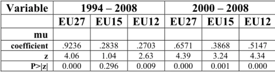
The high values of the mean, µ, of the first part of the cost function’s error, capturing the effects

of the inefficiency, as we defined above, indicates that in all circumstances (see Table 1 below,

with the values taken from Appendix III), technical inefficiencies exist and they are statistically

(12)

11

not be an adequate representation of the data. A more careful observation of the z values

provided in Table 1 allows us to conclude that according to the statistical significance of this

mean, the existence of technical inefficiencies is particularly clear for the time period

2000-2008 and also for the panels that include all EU countries (EU-27) for both time periods

(1994-2008 and 2000-(1994-2008).

TABLE 1 – Summary of the results obtained for the mean, µ

Variable 1994 – 2008 2000 – 2008

EU27 EU15 EU12 EU27 EU15 EU12

mu

coefficient .9236 .2838 .2703 .6571 .3868 .5147 z 4.06 1.04 2.63 4.39 3.24 4.34 P>|z| 0.000 0.296 0.009 0.000 0.001 0.000

The presence of inefficiency is also confirmed by the high values of the contribution of the

inefficiency (u) to the total error. The obtained values of the

2 2

2

v u

u

σ σ

σ γ

+

= , which are reported

in Table 2, reveal that in almost all panels, the inefficient error term amounts to more than 97%.

This implies that in almost all situations, the variation of the total cost among the different EU

countries was due to the differences in their cost inefficiencies. The only exception is the panel

including the newest EU member states (EU-12) for the time period 1994-2000, but the

differences in the cost inefficiency still contributes to 85% of the variation of the total cost.

TABLE 2 – Summary of the results obtained for the contribution of the inefficient

error term to total variance, γ

Variable 1994 – 2008 2000 – 2008

EU27 EU15 EU12 EU27 EU15 EU12

gamma

(13)

12

These results are confirmed by the comparison of the values of the variances of the inefficient

error term (σu) and the random disturbances (σv) which are shown in Table 3. The comparison

of the different columns allows us to conclude that for the EU-27 and EU-15 panels, the

heterogeneity in the entire period (1994-2008) clearly diminishes in the more recent years

(2000-2008). Moreover, in both periods, the EU-12 panel is more homogeneous than the EU-15,

the latter being much more homogeneous than the EU-27 panel.

TABLE 3 – Summary of the results obtained for the variance of the inefficient error term (σu) and the noise (σv)

Variable 1994 – 2008 2000 – 2008

EU27 EU15 EU12 EU27 EU15 EU12

sigma_u2

Coefficient .4973 .1641 .0302 .1957 .0729 .0688 Standard error .2205 .1632 .0191 .0995 .0462713 .0379

sigma_v2

According to the estimation results of the cost function, which are also presented in Appendix

III, we can see that, as expected, the number of the included banks (Z1) increases the total cost.

The same happens with the equity ratio (Z2), while the ratio revenue over expenses decreases

the total cost.

In all situations, the total cost decreases with the trend (t) and increases with the total provided

loans (Y1) and total securities (Y2). With reference to the third output, the “other earning assets”

(Y3), the influence in the total cost is not so clear. Particularly since 2000, the total cost

decreases with these earning assets, but not with its squares (Y3Y3).

On the other hand, the total cost clearly increases with the price of the borrowed funds (W1), but

almost always decreases with the other two inputs, the price of physical capital (W2) and the

(14)

13

inputs in the total cost, we also estimated a simplified model1, in which we include only the

outputs, the inputs and the time trend as explanatory variables. The results obtained are reported

in Appendix IV and they reveal the importance of these variables to the total cost, confirming

the strong and statistically valid positive influence of the price of the borrowed funds on the

total cost and the much clearer positive influence of the price of the physical capital, while the

price of labour still reveals mixed results.

From the residuals of the estimated more complete model (see Appendix III), we also obtain the

country efficiency scores, which are presented in Appendix V. For each panel, the best result is

obtained by the country with the best practice, that is, the country with least waste in its

production process. All the other countries are classified in relation to the panel´s benchmark.

Table 4 below reports the country efficiency rankings by panel and clearly shows that there are

very few changes in the countries’ ranking positions in the different panels.

1

(15)

14

TABLE 4 –Efficiency rankings

EU27 1994-2008

EU27 2000-2008

EU15 1994-2008

EU15 2000-2008

EU12 1994-2008

EU12 2000-2008 Finland Finland Finland Finland Estonia Bulgaria

Sweden Sweden Sweden Luxembourg Lithuania Malta

Luxembourg Luxembourg Luxembourg Sweden Malta Lithuania

Ireland Ireland Ireland Ireland Bulgaria Estonia

Denmark Denmark Denmark Denmark Slovakia Slovakia

Netherlands Netherlands Netherlands Netherlands Latvia Latvia

Belgium Belgium Belgium Belgium Slovenia Slovenia

Italy Italy Italy Italy Romania Cyprus

Spain Spain Spain Spain Cyprus Romania

UK UK UK UK Czech Rep. Czech Rep.

Germany Germany Germany Germany Hungary Poland

France France France France Poland Hungary

Estonia Bulgaria Greece Greece

Bulgaria Lithuania Portugal Portugal

Lithuania Malta Austria Austria

Malta Estonia

Slovakia Slovakia

Latvia Latvia

Romania Slovenia Slovenia Romania Cyprus Cyprus Czech Rep. Czech Rep.

Hungary Hungary

Poland Poland

Greece Greece

Portugal Portugal Austria Austria

The results obtained with the β-Convergence test are presented in Appendix VI and the values

of the estimated β are also reported in Table 5. For almost all panels (the only exception is the

EU-12 panel for the time period 2000-2008), the estimated β are statistically significant and

negative, revealing convergence processes, although these are not very fast, since the values are

relatively small. Nevertheless, the acceleration of the convergence process is very clear during

the last decade (here the period 2000-2008) for all 27 countries and particularly for the

(16)

15

Table 5 – β-Convergence

Variable 1994 – 2008 2000 – 2008

EU27 EU15 EU12 EU27 EU15 EU12

β:

coefficient -.0123885 -.1426132 -.1623192 -.1167656 -.3616606 .0794333 p -4.31 -3.95 -3.21 -2.03 -3.75 1.60 P>|p| 0.000 0.000 0.002 0.044 0.000 0.114

5. Discussion and conclusions

Efficiency is always a concept that relates, in a production function, the allocation of scarce

resources or inputs, with the obtained outputs defining the production possibility frontier. Thus,

technical efficiency will always be a relative measurement of the distance to the frontier,

depending on the definition of the production function and the specific inputs and outputs

included in this function.

One of the advantages of the use of the method of econometric frontiers is that it allows the

decomposition of the deviations from the efficient frontier (the error, ε) between the stochastic

error (the noise, v) and the pure inefficiency (u). Another important advantage is the guarantee

that if we include an irrelevant variable in the function, the econometric frontier method will

detect this irrelevance and the variable will have a very low, or even zero, weight in the

definition of the efficiency results.

However, in spite of these technical advantages, the analysis of bank efficiency always raises

some specific concerns over the definition of the appropriate inputs and outputs to be included

in the production function.

In this paper, we opt to use the intermediation approach and, taking into account the specific

character of the bank production activities and the available data, we define a cost frontier

(17)

16

prices of three inputs (borrowed funds, physical capital and labour). We also include three other

variables that may influence the efficiency results, namely, the number of banks, the equity ratio

and the ratio revenue over expenses.

Our data are taken from the Bankscope database, which is recognised as one of the best sources,

since it includes data for all EU countries and guarantees standardisation and comparability,

providing data on banks accounting for around 90% of total assets. Nevertheless, Bankscope

data can still be very unbalanced, at least in the number of included banks. Our Appendix I

clearly shows that around 30% of the included banks are from one country (Germany) and the

banks of four countries (Germany, France, Italy and UK) account for half of the banks

considered. On the other hand, while it is true that the number of banks can be important, we

should also take into account their weight and the degree of concentration in the specific bank

market.

With regard to the variables, Bankscope does not directly provide the prices of the production

inputs. Therefore, we consider proxies of these prices; specifically, for the price of the borrowed

funds, we took the ratio interest expense over the sum of deposits, for physical capital, the ratio

of the non-interest expenses over fixed assets and for the price of labour, the ratio personnel

expenses over the number of employees.

For all panels, our estimations point to the dominance of the borrowed funds to explain the

evolution of the total cost and the relatively low weight of the other two inputs (physical capital

and labour), which reveal a mixed and unclear influence on the cost. This confirms the

intermediation approach and the very specific characteristics of the banks’ production process,

since it depends much more on the borrowed funds than on the traditional production factors.

On the other hand, with regard to the influence of the considered outputs in the total cost, the

validation of the intermediation approach is reinforced as total cost clearly always grows in line

(18)

17

provided total securities will contribute to the growth of the total cost, while the influence of the

other earning assets (here, the difference between the total earning assets and the total loans) is

not so clear. However, taking into particular account the results obtained with the simplified

model (Appendix IV), we can also conclude that total cost positively depends on the increase of

the other earning assets.

As expected, the total cost always increases with the growth of the considered banks and the

equity ratio (a possible proxy for the accepted risk) and decreases with the ratio revenue over

expenses. Furthermore, in all situations the time trend variable, which can be interpreted as the

neutral technological changes, clearly contributes to the decrease of the total cost.

Our results also very clearly point to the existence of statistically important technical

inefficiency in all panels, although this appears to decline in recent years (2000-2008), once

again in all panels. Regarding the obtained ranking positions, there are very few changes in the

efficiency rankings of the EU countries.

Moreover, the obtained results confirm the existence of a convergence process, but in spite of

the clear acceleration of this process during the last decade (2000-2008), it is still quite slow and

does not raise any credible prospects of full integration being achieved in the near future.

These results do not allow us to support the validity of the Law of One Price in the European

bank markets. In an increasingly competitive environment, the ability to create differentiated

products is crucial and financial products have become increasingly complex, so that market and

(19)

18

References

Affinito, M. and Farabullini, F. (2009) “Does the Law of One Price hold in Euro-Area Retail

Banking? An Empirical Analysis of Interest Rate Differentials across the Monetary Union” International

Journal of Central Banking, 5, pp. 5-37.

Aigner, D., Lovell C.A.K. and Schmidt, P. (1977) “Formulation and estimation of stochastic frontier

production function models”, Journal of Econometrics, 6, pp. 21-37.

Allen, F. and Gale, D. (1997) “Financial Markets, Intermediaries and Inter-temporal Smoothing”

Journal of Political Economy, 105, pp. 523-546.

Altunbas, Y., Gardener, E.P.M., Molyneux, P. and Moore, B. (2001) “Efficiency in European

banking” European Economic Review, 45, pp. 1931-1955.

Altunbas, Y. and Marquês, D. (2008) “Mergers and acquisitions and bank performance in Europe.

The role of strategic similarities”, Journal of Economics and Business, 60, pp. 204-222.

Arghyrou, M.G., Gregoriou, A. and Kontonikas, A. (2009) “Do real interest rates converge?

Evidence from the European union”, Journal of International Financial Markets, Institutions & Money, 19,

pp. 447-460.

Baele, L., Ferrando, A., Hordahl, P., Krylova, E. and Monnet, C. (2004) “Measuring European

Financial Integration”, Oxford Review of Economic Policy, 20, pp. 509-530.

Barro, R. J. and Sala-i-Martin, X. (1992) “Convergence” Journal of Political Economy, 100, pp.

223-251.

Barros, C., Ferreira, C. and Williams, J. (2007) “Analysing the determinants of performance of

best and worse European banks: A mixed logit approach”, Journal of Banking and Finance, 31, pp.

2189-2203.

Battese, G. E. and Coelli, T. J. (1988) “Prediction of firm-level technical efficiencies with a

generalized frontier production function and panel data”, Journal of Econometrics, 38, pp. 387-399.

Battese, G. E. and Coelli, T. J. (1992) “Frontier Production Functions, Technical Efficiency and

Panel Data: With Application to Paddy Farmers in India”, Journal of Productivity Analysis, 3, pp. 153-169.

Battese, G. E. and Coelli, T. J.(1995) “A Model for Technical Inefficiency Effects in a Stochastic

Frontier Production Function for Panel data”, Empirical Economics, 20, pp. 325-332.

Battese, G., Coelli, T. J. and Colby, T. (1989) “Estimation of Frontier Production Functions and

the Efficiencies of Indian Farms Using Panel Data from ICRISTAT’s Village Level Studies,” Journal of

Quantitative Economics, 5, pp. 327-348.

Beck, T., Demirguç-Kunt, A. and Levine, R. (2003-a) “Law, endowments, and finance”, Journal

of Financial Economics, 70, 137–181.

Beck, T., Demirguç-Kunt, A. and Levine, R. (2003-b) “Law and finance. Why does legal origin

matter?” Journal of Comparative Economics, 31, 653–675.

Berger, A. N. (2003) “The economic effects of technological progress: Evidence from the banking

industry”, Journal of Money, Credit and Banking, 35, pp. 141-176.

Berger, A. N. (2007) “International Comparisons of Banking Efficiency”, Financial Markets,

Institutions and Instruments, 16, pp. 119-144.

Berger, A.N., DeYoung, R. and Udell, G.F. (2001) “Efficiency barriers to the consolidation of the

European Financial services industry” European Financial Management, 7, pp. 117-130.

Berger, A.N. and Humphrey, D. B. (1991) “The dominance of inefficiencies over scale and

(20)

19

Berger, A.N. and Mester, L. J. (1997) “Inside the black box: What explains differences in

inefficiencies of financial institutions?”, Journal of Banking and Finance, 21, pp. 895-947.

Bikker, J.A., Spierdijk, L. and Finnie, P. (2006) The impact of bank size on market power,

Netherlands Central Bank, Research Department, DNB Working Paper No. 120,

Bonin, J.P., Hasan, I. and Wachtel, P. (2005) “Bank performance, efficiency and ownership in

transition countries” Journal of Banking and Finance, 29, pp. 31-53.

Bos, J. W. B. and Kool, C. J. M. (2006) “Bank efficiency: The role of bank strategy and local

market conditions” Journal of Banking and Finance, 30, pp. 1953-1974.

Bos, J. W. B. and Schmiedel, H. (2007) “Is there a single frontier in a single European

banking market?” Journal of Banking and Finance, 31, pp. 2081-2102.

Cabral I., Dierick, F. and Vesala, J. (2002) Banking Integration in the Euro Area, ECB Occasional

Paper Series No. 6.

Campa, J.M. and Hernando, I. (2006) “M&As performance in the European financial industry”,

Journal of Banking and Finance, 30, pp. 3367-3392.

Cappiello, L., Hodahl, P., Kadareja, A. and Manganelli, S. (2006) The impact of the euro on

financial markets, ECB Working Paper Series No. 598.

Casu, B., Girardone, C. and Molyneux, P. (2004) “Productivity change in European banking: A

comparision of parametric and non-parametric approaches”, Journal of Banking and Finance, 28, pp.

2521-2540.

Casu, B. and Girardone, C. (2009) “Competition issues in European banking” Journal of Financial

Regulation and Compliance, 17, pp. 119-133.

Casu, B. and Girardone, C. (2010) “Integration and efficiency convergence in EU banking

markets” Omega, 38, pp. 260-267.

Coelli, T., D., Rao, D. S. P. , O’Donnell, C. J. and Battese, G. E. (2005) An introduction to

efficiency and productivity analysis, 2nd. Ed. Springer Science+Business Media, Inc., New York.

Dermine, J. (2006) “European banking integration: Don’t put the cart before the horse”, Financial

Markets, Institutions and Instruments, 15, pp. 57-106.

Diaz, B. D.,. Olalla, M. G. and Azofra, S. S. (2004) “Bank acquisitions and performance:

evidence from a panel of European credit entities” Journal of Economics and Business, 56, pp. 377-404.

European Central Bank (2003) “The integration of Europe’s financial markets” in ECB Monthly

Bulletin, October 2003, pp. 53-66.

European Central Bank (2007) Financial integration in Europe, ECB, Frankfurt.

European Central Bank (2008) Financial integration in Europe, ECB, Frankfurt.

Farrell, M.J. (1957) “The Measurement of Productive Efficiency” Journal of the Royal Statistical

Society, 120, pp. 253-290.

Frerier, G.D. and Lowell, C.A.K. (1990)” Measuring cost efficiency in banking: Econometric and

linear programming evidence”, Journal of Econometrics46, pp. 229-245.

Gardener, E.P.M., Molyneux, P. and Moore, B. (ed.) (2002) - Banking in the New Europe – The

Impact of the Single Market Program and EMU on the European Banking Sector, Palgrave, Macmillan.

Greene, W.M. (1990) “A gamma-distributed stochastic frontier model”, Journal of Econometrics,

46, pp. 141-163.

(21)

20

Greene, W.M. (2008)“The econometric approach to efficiency analysis”. In: Fried, H.O., Lovell,

C.A.K. and Schmidt, P. (Eds.), The Measurement of Productive Efficiency: Techniques and Applications,

Oxford University Press, Oxford, pp. 92-251.

Goddard, J.A., Molyneux, P. and Wilson, J. O. S. (2001) European banking efficiency, technology

and growth, John Willey and Sons.

Goddard, J.A., Molyneux, P., and Wilson, J. O. S. (2007) “European banking: an overview”,

Journal of Banking and Finance, 31, pp. 1911-1935.

Gropp, R. and Kashyap, A. K. (2010) “A New Metric for Banking Integration in Europe”, in Alesina,

A. and Giavazzi, F. (ed.) Europe and the Euro, NBER Books, National Bureau of Economic Research, pp.

219-246.

Guiso, L., Jappelli, T., Padula, M. and Pagano, M. (2004) “Financial market integration and

economic growth in the EU”, Economic Policy, 40, pp. 523-577.

Hartmann P., Maddaloni, A. and Manganelli, S. (2003) “The euro area financial system: structure

integration and policy initiatives” Oxford Review of Economic Policy, 19, pp. 180-213.

Holló, D. and Nagy, M. (2006) “Bank Efficiency in the enlarged European Union” in The banking

system in emerging economies: how much progress has been made?,BIS Papers, N. 28, Bank of International

Settlements Papers, Monetary and Economic Department, pp. 217-235.

Hughes, J. P. and Mester, L. J. (2008) Efficiency in banking: theory, practice and evidence, Federal

Reserve Bank of Philadelphia, Working Paper 08-1.

Jondrow, J., Lovell, C.A.K., Materov, I.S. and Schmidt, P. (1982) “On estimation of technical

inefficiency in the stochastic frontier production function model”, Journal of Econometrics, 19, pp. 233-238.

Kasman, A. and Yildirim, C. (2006) “Cost and profit efficiencies in transition banking: the

case of new EU members”, Applied Economics, 38 pp. 1079-1090.

Kumbhakar, S.C. and Lovell, C.A.K. (2000) Stochastic Frontier Analysis, Cambridge University

Press, Cambridge.

Kumbhakar, S.C., Lozano-Vivas, A., Lovell, C.A.K. and Hasan, I. (2001) “The effects of

deregulation on the performance of financial institutions: The case of Spanish savings banks”, Journal of

Money, Credit and Banking, 33, pp. 101-120.

Lamont, O. A. and Thaler, R. H. (2003) “Anomalies: The Law of One Price in Financial Markets”,

Journal of Economic Perspectives, 17, pp. 191-202.

Lensink, R., Meesters, A. and Naaborg, I. (2008) “Bank efficiency and foreign ownership: Do good

institutions matter” Journal of Banking and Finance, 32, pp. 834-844.

Manna, M. (2004) Developing statistical indicators of the integration of the euro area banking

system, ECB Working Paper Series No.300.

Meeusen, W. and van den Broeck, J. (1977) “Efficiency estimation from a Cobb-Douglas

production function with composed error” International Economic Review, 18, pp. 435-444.

Molyneux, P. (2003) “Does size matter?” Financial restructuring under EMU, United Nations

Universiy, Institute for New Technologies, Working Paper No. 03-30.

Murinde, V., Agung, J. and Mullineux, A. W. (2004) “Patterns of corporate financing and

financial system convergence in Europe”, Review of International Economics, 12, pp. 693-705.

Quah, D. (1996) “Twin peaks: growth and convergence in models of distribution dynamics”,

(22)

21

Resti, A. (1997) “Evaluating the cost-efficiency of the Italian banking system: what can be learn

from the joint application of parametric and non-parametric techniques”, Journal of Banking and Finance,

21, pp. 221-250.

Rossi, S., M. Schwaiger and G. Winkler (2005) Managerial Behaviour and Cost/Profit Efficiency

in the Banking Sectors of Central and Eastern European Countries, Oesterreichische Nationalbank

(Austrian Central Bank) Working Paper 96.

Schaeck, K. and Cihak, M. (2007) Bank competition and capital ratio, IMF Working Paper

WP/07/216.

Schure, P., Wagenvoort, R. and O’Brien, D. (2004) “The efficiency and the conduct of European

banks: Developments after 1992” Review of Financial Economics, 13, pp.371–396.

Sealey, C.W. Jr. and Lindley, J. T. (1977) “Inputs, outputs and a theory of production and cost at

depository financial institution” Journal of Finance, 32, pp. 1251–1266.

Sørensen, C. K. and Gutiérrez, J. M. P. (2006) Euro area banking sector integration using

hierarchical cluster analysis techniques, ECB Working Paper Series No. 627.

Stevenson, R. F. (1980) “Likelihood Functions for Generalized Stochastic Frontier Estimation”,

Journal of Econometrics, 13, pp. 57-66.

Sturm, J-E and Williams, B. (2010) “What determines differences in foreign bank efficiency?

Australian evidence”, Journal of International Financial Markets, Institutions and Money, 20, pp.

284-309.

Tortosa-Ausina, E. (2002) “Exploring efficiency differences over time in the Spanish banking

industry”, European Journal of Operational Research, 139, pp. 643-664.

Vives, X. (2001) – “Restructuring Financial Regulation in the European Monetary Union”,

Journal of Financial Services Research, 19, pp. 57-82.

Weill L. (2004), “Measuring Cost Efficiency in European Banking: A comparison of frontier

techniques”, Journal of Productivity Analysis, 21, 133-152.

Weill, L. (2009) “Convergence in banking efficiency across European countries”, Journal of

International Financial Markets Institutions and Money, 19, pp. 818-833.

Wheelock, D.C. and Wilson, P. W. (1999) “Technical progress, inefficiency and productivity

change in US banking, 1984-1993” Journal of Money, Credit and Banking, 31, pp. 213-234.

Williams, J. and Nguyen, N. (2005) “Financial liberalisation, crisis and restructuring: A

comparative study of bank performance and bank governance in South East Asia”, Journal of Banking and

(23)

22

APPENDIX I – Panel stochastic frontier models

For panel data models, and particularly with stochastic frontier models, it is necessary not only to suppose the normality for the noise error term (v) and half- or truncated normality for the inefficiency error term (u), but also to assume that the firm specific level of inefficiency is uncorrelated with the input levels. This type of model also addresses the fundamental question of how and whether inefficiencies vary over time.

Following Battese and Coelli (1988) and Battese et al. (1989), a general panel stochastic frontier model, with Ti time observations of i units, can be represented as:

[

]

[ ]

2 2 , 0 ~ , ~ v it u i i it it it T it N v N u u v x Y σ σ µ β

α + + −

=

Using the Greene (2003) reparameterisation and the truncated normal distribution of ui, we have

[

]

(

)( )

2 2 * 2 2 * , 2 , 1 , 1 1 1 * * * * * * ,..., , u i i v u i i it T it it i i i i i i i i i i T i i i i T x y u E i

σ

γ

σ

λ

γ

αβ

ε

γ

µ

γ

µ

σ

µ

σ

µ

φ

σ

µ

ε

= = + = − = − − + =                  − Φ       + =

(24)

23

APPENDIX II – Number of banks (and %) by country

Country 1994 2000 2008 Average

(1994-2008)

Austria 54 (2.34) 129 (4.92) 147 (6.92) 127 (4.90)

Belgium 88 (3.82) 68 (2.60) 34 (1.60) 72 (2.78)

Bulgaria 10 (0.43) 25 (0.95) 21 (0.99) 23 (0.89)

Cyprus 12 (0.52) 23 (0.88) 9 (0.42) 18 (0.69)

Czech Rep. 24 (1.04) 27 (1.03) 20 (0.94) 26 (1.00)

Denmark 98 (4.25) 123 (4.69) 109 (5.13) 116 (4.48)

Estonia 9 (0.39) 10 (0.38) 10 (0.47) 11 (0.42)

Finland 11 (0.48) 14 (0.53) 12 (0.56) 13 (0.50)

France 350 (15.18) 308 (11.76) 204 (9.60) 297 (11.46)

Germany 786 (34.08) 771 (29.43) 593 (27.92) 738 (28.48)

Greece 25 (1.08) 26 (0.99) 29 (1.37) 32 (1.24)

Hungary 30 (1.30) 39 (1.49) 26 (1.22) 34 (1.31)

Ireland 24 (1.04) 42 (1.60) 40 (1.88) 42 (1.62)

Italy 177 (7.68) 216 (8 .24) 199 (9.37) 231 (8.92)

Latvia 16 (0.69) 25 (0.95) 33 (1.55) 27 (1.04)

Lithuania 7 (0.30) 16 (0.61) 15 (0.71) 14 (0.54)

Luxembourg 118 (5.12) 112 (4.27) 80 (3.77) 106 (4.09)

Malta 8 (0.35) 10 (0.38) 14 (0.66) 12 (0.46)

Netherlands 50 (2.17) 50 (1.91) 41 (1.93) 57 (2.20)

Poland 33 (1.43) 50 (1.91) 37 (1.74) 48 (1.85)

Portugal 34 (1.47) 37 (1.41) 25 (1.18) 36 (1.39)

Romania 3 (0.13) 31 (1.18) 27 (1.27) 23 (0.89)

Slovakia 11 (0.48) 22 (0.84) 16 (0.75) 19 (0.73)

Slovenia 14 (0.61) 25 (0.95) 21 (0.99) 23 (0.89)

Spain 172 (7.46) 204 (7.79) 136 (6.40) 196 (7.56)

Sweden 14 (0.61) 22 (0.84) 78 (3.67) 60 (2.32)

UK 128 (5.55) 195 (7.44) 148 (6.97) 190 (7.33)

TOTAL 2306 2620 2124 2591

APPENDIX III – Estimates with Cost Frontier Function

Variable 1994 – 2008 2000 – 2008

EU27 EU15 EU12 EU27 EU15 EU12

Constant:

coefficient 4.5533 4.7331 7.9005 10.641 1.4500 8.2714 z 6.20 4.60 5.17 6.16 0.48 2.12 P>|z| 0.000 0.000 0.000 0.000 0.634 0.034

Y1:

coefficient .3304 .3279 .0447 .1061 1.0492 .6560 z 2.13 1.08 0.16 0.42 1.63 1.63 P>|z| 0.033 0.279 0.874 0.671 0.104 0.102

Y2:

coefficient .0444 .3906 .0245 1.1363 1.6670 .7928 z 0.26 0.82 0.10 3.15 2.14 1.41 P>|z| 0.796 0.412 0.917 0.002 0.032 0.158

Y3:

coefficient .0493 -.1399 .0639 -1.3520 -1.6713 -1.3663 z 0.21 -0.24 0.18 -2.77 -1.63 -1.87 P>|z| 0.836 0.807 0.856 0.006 0.103 0.062

W1:

coefficient .6541 1.4086 .0269 1.6380 1.8361 .3792 z 4.64 4.95 0.11 6.12 4.66 0.61 P>|z| 0.000 0.000 0.913 0.000 0.000 0.541

W2:

(25)

24

W3:

coefficient -.0496 -.1763 -.6446 .5571 -.5339 .1188 z -0.95 -2.70 -3.67 4.60 -1.88 0.29 P>|z| 0.343 0.007 0.000 0.000 0.060 0.773

Y1Y1:

coefficient .0431 .0253 .0373 .0673 .0597 .0715 z 2.62 0.81 1.85 3.46 1.74 2.60 P>|z| 0.009 0.418 0.064 0.001 0.082 0.009

Y1Y2:

coefficient .0633 .1055 .0533 .0030 -.0139 -.0687 z 2.57 1.51 1.94 0.09 -0.13 -2.02 P>|z| 0.010 0.132 0.053 0.927 0.898 0.044

Y1Y3:

coefficient -.1438 -.1737 -.1076 -.1076 -.1498 -.0934 z -3.74 -1.95 -2.27 -2.23 -1.15 -1.65 P>|z| 0.000 0.052 0.023 0.026 0.252 0.099

Y2Y2:

coefficient .0025 -.1381 .0107 .0265 .2420 .0540 z 0.22 -1.62 0.84 1.47 2.08 2.91 P>|z| 0.828 0.106 0.402 0.141 0.037 0.004

Y2Y3:

coefficient -.0714 .1515 -.0660 -.1079 -.5395 -.0681 z -2.27 0.85 -1.76 -2.39 -2.04 -1.32 P>|z| 0.023 0.393 0.078 0.017 0.042 0.188

Y3Y3:

coefficient .1201 .0368 .0959 .1486 .3938 .1291 z 3.81 0.33 2.40 3.34 2.18 2.53 P>|z| 0.000 0.739 0.016 0.001 0.029 0.012

W1W1:

coefficient .0056 .0384 .0386 .0955 .0702 .0534 z 0.40 1.07 2.38 4.95 1.90 1.94 P>|z| 0.688 0.285 0.017 0.000 0.057 0.053

W1W2:

coefficient .0441 .0655 -.0118 .0804 .0446 -.0112 z 2.15 2.18 -0.39 3.09 1.24 -0.18 P>|z| 0.031 0.029 0.698 0.002 0.217 0.859

W1W3:

coefficient .0029 .0225 .0112 .0064 .0331 .0160 z 0.45 1.71 0.78 0.61 1.65 0.48 P>|z| 0.650 0.088 0.436 0.543 0.099 0.632

W2W2:

coefficient -.0393 -.1110 .0099 -.0157 -.0482 -.0021 z -2.60 -5.64 0.41 -0.72 -1.50 -0.04 P>|z| 0.009 0.000 0.682 0.472 0.133 0.971

W2W3:

coefficient .0070 -.0446 .0280 -.0305 .0006 -.0252 z 0.80 -2.80 1.74 -2.24 0.02 -0.46 P>|z| 0.423 0.005 0.082 0.025 0.983 0.643

W3W3:

coefficient -.0030 -.0062 -.0075 .0082 -.0182 -.0106 z -1.73 -2.26 -1.23 2.66 -2.38 -0.95 P>|z| 0.083 0.024 0.220 0.008 0.017 0.341

Y1W1:

coefficient -.0283 -.1721 .0145 -.0045 -.1058 .0465 z -1.41 -4.02 0.59 -0.17 -2.28 1.07 P>|z| 0.157 0.000 0.558 0.866 0.023 0.285

Y1W2:

coefficient -.0114 .0825 -.0796 .0597 .1085 .0129 z -0.49 2.54 -2.32 2.04 2.99 0.22 P>|z| 0.625 0.011 0.020 0.041 0.003 0.828

Y1W3:

coefficient -.0050 .0178 .0600 -.0158 .0472 .0444 z -0.68 1.29 3.75 -1.47 1.55 1.32 P>|z| 0.500 0.198 0.000 0.142 0.120 0.186

Y2W1:

coefficient .0118 .1485 -.0206 .1290 .1155 .0270 z 0.52 2.03 -0.77 2.82 1.45 0.39 P>|z| 0.603 0.043 0.442 0.005 0.148 0.697

Y2W2:

(26)

25 z -3.15 -4.47 -1.13 -3.68 -0.42 -1.82

P>|z| 0.002 0.000 0.258 0.000 0.672 0.069

Y2W3:

coefficient -.0050 -.0298 -.0776 .0482 .0328 -.0190 z -0.52 -1.32 -3.40 2.82 0.80 -0.31 P>|z| 0.606 0.188 0.001 0.005 0.421 0.754

Y3W1:

coefficient .0128 -.0102 .0517 -.1496 -.0589 -.0431 z 0.42 -0.12 1.35 -2.92 -0.63 -0.54 P>|z| 0.671 0.904 0.176 0.003 0.527 0.591

Y3W2:

coefficient .1327 .2113 .1555 .1609 -.0633 .1874 z 3.07 2.85 2.45 3.04 -0.54 2.36 P>|z| 0.002 0.004 0.014 0.002 0.593 0.018

Y3W3:

coefficient .0128 .0258 .0565 -.0649 -.0395 -.0268 z 0.93 1.09 1.91 -3.05 -0.76 -0.40 P>|z| 0.350 0.276 0.057 0.002 0.450 0.692

Z1:

coefficient .0082 .0127 .1095 .0101 .0162 .0486 z 0.44 0.70 3.16 0.46 0.58 1.23 P>|z| 0.662 0.485 0.002 0.643 0.563 0.218

Z2:

coefficient .0647 .1703 .0343 .1589 .1265 -.0256 z 2.76 3.85 1.11 4.06 2.41 -0.46 P>|z| 0.006 0.000 0.266 0.000 0.016 0.648

Z3:

coefficient -.7141 -.9609 -.4682 -.5947 -.6249 -.3441 z -10.37 -7.83 -5.88 -7.47 -5.10 -3.39 P>|z| 0.000 0.000 0.000 0.000 0.000 0.001

t:

coefficient -.0048 -.0081 -.0050 -.0224 -.0212 -.0010 z -1.80 -2.21 -0.98 -5.95 -6.35 -0.48 P>|z| 0.072 0.027 0.329 0.000 0.000 0.633

mu

coefficient .9236 .2838 .2703 .6571 .3868 .5147

z 4.06 1.04 2.63 4.39 3.24 4.34

P>|z| 0.000 0.296 0.009 0.000 0.001 0.000

lnsigma2

coefficient -.6859 -1.7873 -3.3358 -1.6154 -2.5925 -2.6451

z -1.57 -1.83 -6.23 -3.23 -4.20 -4.96

P>|z| 0.117 0.067 0.000 0.001 0.000 0.000

ilgtgamma

coefficient 4.3682 3.8951 1.7286 4.1601 3.6285 3.4378

z 9.67 3.83 2.68 7.70 5.47 5.94

P>|z| 0.000 0.000 0.007 0.000 0.000 0.000

sigma2

gamma

sigma_u2

sigma_v2

(27)

26 Log likelihood 361.60132 278.76336 190.12184 277.52094 189.10569 144.04883

N 405 225 180 243 135 108

(*) TC = Total cost (dependent variable) = natural logarithm of the sum of the interest expenses plus the total operating expenses

Outputs: Y1 = Total loans = natural logarithm of the loans

Y2 = Total securities = natural logarithm of the total securities

Y3 = Other earning assets= natural logarithm of difference between the total earning assets and the total

loans

Inputs:W1 = Price of the borrowed funds = natural logarithm of the ratio interest expenses over the sum of deposits;

W2 = Price of physical capital = natural logarithm of the ratio non-interest expenses over fixed assets

W3 = Price of labour = natural logarithm of the ratio personnel expenses over the number of employees

Other variables:Z1 = Number of banks= natural logarithm of the number of banks included in the panels

Z2 = Equity ratio = natural logarithm of the ratio equity over total assets

Z3 = Ratio revenue over expenses = natural logarithm of the ratio of the total revenue over the total

expenses

t = time trend

APPENDIX IV – Estimates with Cost Frontier Function (simplified model)

Variable 1994 – 2008 2000 – 2008

EU27 EU15 EU12 EU27 EU15 EU12

Constant:

coefficient 1.704008 1.436849 3.725444 1.508172 -.4157846 4.894205 z 8.93 5.47 10.23 4.93 -1.05 11.22 P>|z| 0.000 0.000 0.000 0.000 0.295 0.000

Y1:

coefficient .4575199 .5483316 .3794408 .5693051 .7773747 .4458871 z 28.35 20.18 16.27 30.25 19.68 19.60 P>|z| 0.000 0.000 0.000 0.000 0.000 0.000

Y2:

coefficient .0231095 .0334319 .0276436 -.0117959 -.1326427 .0379789 z 1.31 0.73 1.37 -0.54 -2.61 1.72 P>|z| 0.190 0.463 0.172 0.590 0.009 0.085

Y3:

coefficient .3180318 .2530069 .3485391 .254392 .3151639 .1929269 z 11.80 4.50 10.09 7.39 4.16 4.64 P>|z| 0.000 0.000 0.000 0.000 0.000 0.000

W1:

coefficient .5813181 .5953075 .6232564 .5896733 .6100655 .5941992 z 35.40 26.52 25.73 33.46 26.12 26.56 P>|z| 0.000 0.000 0.000 0.000 0.000 0.000

W2:

coefficient .0371296 -.0254601 .1145439 .0708342 .0877214 .1673463 z 1.82 -1.01 3.67 2.74 2.71 4.00 P>|z| 0.069 0.313 0.000 0.006 0.007 0.000

W3:

coefficient -.008435 .0031862 -.0315724 .0157908 -.0229858 .0270339 z -1.10 0.38 -2.76 1.34 -1.52 1.85 P>|z| 0.270 0.705 0.006 0.179 0.128 0.065

t:

(28)

27 P>|z| 0.146 0.013 0.029 0.000 0.000 0.896

mu

coefficient 1.114109 -.0998493 .5355472 1.181618 .4111179 .4174215

z 4.93 -0.08 4.03 6.19 1.58 1.99

P>|z| 0.000 0.935 0.000 0.000 0.114 0.047

lnsigma2

Coefficient -.5008453 -.3119287 -2.592984 -.8834989 -1.615981 -1.942696

z -1.23 -0.27 -6.22 -2.27 -2.17 -2.74

P>|z| 0.219 0.787 0.000 0.023 0.030 0.006

ilgtgamma

coefficient 3.905836 4.640099 1.504086 4.208388 3.778475 3.321973

z 9.21 3.95 2.87 10.08 4.75 4.41

P>|z| 0.000 0.000 0.004 0.000 0.000 0.000

sigma2

gamma

sigma_u2

sigma_v2

Wald chi2(31) 8183.79 4101.42 5143.74 4559.79 2142.34 3690.80 Prob > chi2 0.0000 0.0000 0.0000 0.0000 0.0000 0.0000

Log likelihood 237.26571 194.54221 106.63578 191.7829 134.0707 102.92957 N 405 225 180 243 135 108

(*) TC = Total cost (dependent variable) = natural logarithm of the sum of the interest expenses plus the total operating expenses

Outputs: Y1 = Total loans = natural logarithm of the loans

Y2 = Total securities = natural logarithm of the total securities

Y3 = Other earning assets= natural logarithm of the difference between the total earning assets and the

total loans

Inputs:W1 = Price of the borrowed funds = natural logarithm of the ratio interest expenses over the sum of deposits;

W2 = Price of physical capital = natural logarithm of the ratio non-interest expenses over fixed assets

W3 = Price of labour = natural logarithm of the ratio personnel expenses over the number of employees

(29)

28

APPENDIX V – Cost efficiency rankings

A – EU-27

EU27 1994 - 2008 EU27 2000 - 2008

1 Finland 100.000 Finland 100.000

2 Sweden 98.947 Sweden 98.917

3 Luxembourg 98.935 Luxembourg 98.913

4 Ireland 98.924 Ireland 98.892

5 Denmark 98.886 Denmark 98.848

6 Netherlands 98.838 Netherlands 98.801

7 Belgium 98.830 Belgium 98.785

8 Italy 98.818 Italy 98.763

9 Spain 98.792 Spain 98.746

10 UK 98.774 UK 98.731

11 Germany 98.772 Germany 98.728

12 France 98.715 France 98.668

13 Estonia 98.699 Bulgaria 98.581 14 Bulgaria 98.684 Lithuania 98.579 15 Lithuania 98.681 Malta 98.578

16 Malta 98.662 Estonia 98.572

17 Slovakia 98.642 Slovakia 98.563

18 Latvia 98.618 Latvia 98.526

19 Romania 98.599 Slovenia 98.502 20 Slovenia 98.594 Romania 98.491

21 Cyprus 98.580 Cyprus 98.490

22 Czech Rep. 98.535 Czech Rep. 98.446

23 Hungary 98.503 Hungary 98.392

24 Poland 98.491 Poland 98.390

25 Greece 98.397 Greece 98.303

26 Portugal 98.389 Portugal 98.286

27 Austria 98.351 Austria 98.262

average 98.728 98.658

median 98.684 98.579

stand. dev. 0.299 0.324

B – EU-15

EU15 1994 - 2008 EU15 2000 - 2008

1 Finland 100.000 Finland 100.000 2 Sweden 98.933 Luxembourg 98.944 3 Luxembourg 98.911 Sweden 98.924

4 Ireland 98.899 Ireland 98.914

5 Denmark 98.858 Denmark 98.858

6 Netherlands 98.819 Netherlands 98.826

7 Belgium 98.795 Belgium 98.806

8 Italy 98.779 Italy 98.781

9 Spain 98.773 Spain 98.768

10 UK 98.751 UK 98.752

11 Germany 98.744 Germany 98.748

12 France 98.678 France 98.687

13 Greece 98.324 Greece 98.286

(30)

29

15 Austria 98.271 Austria 98.240

average 98.791 98.787

median 98.779 98.781

stand. dev. 0.386 0.397

C – EU-12

EU12 1994 - 2008 EU12 2000 - 2008

1 Estonia 100.000 Bulgaria 100.000 2 Lithuania 98.999 Malta 98.998 3 Malta 98.997 Lithuania 98.997 4 Bulgaria 98.996 Estonia 98.989 5 Slovakia 98.975 Slovakia 98.982

6 Latvia 98.951 Latvia 98.962

7 Slovenia 98.936 Slovenia 98.947 8 Romania 98.934 Cyprus 98.944 9 Cyprus 98.930 Romania 98.938 10 Czech Rep. 98.892 Czech Rep. 98.908 11 Hungary 98.860 Poland 98.880 12 Poland 98.859 Hungary 98.876

average 99.027 99.035

median 98.943 98.955

stand. dev. 0.297 0.294

APPENDIX VI – β-Convergence estimates

Variable (*) 1994 – 2008 2000 – 2008

EU27 EU15 EU12 EU27 EU15 EU12

Constant:

coefficient .1217614 .35908 .4342104 .2965211 1.020656 -.2046035 p 4.48 4.09 3.24 2.06 3.76 -1.55 P>|p| 0.000 0.000 0.001 0.041 0.000 0.126

β:

coefficient -.0123885 -.1426132 -.1623192 -.1167656 -.3616606 .0794333 p -4.31 -3.95 -3.21 -2.03 -3.75 1.60 P>|p| 0.000 0.000 0.002 0.044 0.000 0.114

R-squared 0.1615 0.1173 0.1849 0.0973 0.1623 0.1542

N 378 210 168 216 210 96