MBE_Woollett_MaximaSolve.pdf

(1)

Maxima by Example: Ch.4: Solving Equations

∗

Edwin L. Woollett

January 29, 2009

4 Solving Equations

Maxima has several functions which can be used for solving sets of algebraic equations and for nding the roots of an expression. These are described in the Maxima manual, Sec. 21, and listed under Contents under Equations.

This chapter gives examples of the following Maxima functions:

• solve solves a system of simultaneous linear or nonlinear polynomial equations for the specied

vari-able(s) and returns a list of the solutions.

• linsolve solves a system of simultaneous linear equations for the specied variables and returns a list of

the solutions.

• nd root uses a combination of binary search and Newton-Raphson methods for univariate functions

and will nd a root when provided with an interval containing at least one root.

• allroots nds all the real and complex roots of a real univariate polynomial.

• realroots nds all of the real roots of a univariate polynomial within a specied tolerance. • eliminate eliminates variables from a set of equations or expressions.

• linsolve by lu solves a system of linear algebraic equations by the matrix method known as LU

decom-position, and provides a Maxima method to work with a set of linear equations in terms of the matrix of coefcients.

• newton, naive univariate Newton-Raphson, and mnewton, multivariate Newton-Raphson, can deal with

nonlinear function(s).

We also encourage the use of two dimensional plots to approximately locate solutions.

This chapter does not yet include Solving Recurrence Relations, and Solving One Hundred Equations.

4.1 One Equation or Expression: Symbolic Solution or Roots

4.1.1 The Maxima Function solve

Maxima's ability to solve equations is limited, but progress is being made in this area. The Maxima man-ual has an extensive entry for the important function solve, which you can view in Maxima with the input ? solve (no semicolon) followed by (Enter), or the equivalent command: describe(solve)$. The in-put example(solve)$ will show you the manual examples without the manual syntax material. We will present some examples of the use of solve and not try to cover everything.

solve tries to nd exact solutions. If solve(f(x),x) cannot nd an exact solution, solve tries to return a simplied version of the original problem. Sometimes the simplied version can be useful:

(%i1) f(x);

(%o1) f(x)

(%i2) solve( f(x)2-1 , x );

(%o2) [f(x) = - 1, f(x) = 1]

(4)

The Maxima manual solve syntax discussion relevant to solving one equation is:

Function: solve(expr, x) Function: solve(expr)

Solves the algebraic equation expr for the variable x and returns a list of solution equations in x. If expr is not an equation, the equation expr = 0 is assumed in its place. x may be a function (e.g. f(x)), or other non-atomic expression except a sum or product. x may be omitted if expr contains only one variable. expr may be a rational expression, and may contain trigonometric functions, exponentials, etc.

breakup if false will cause solve to express the solutions of cubic or quartic equations as single expressions rather than as made up of several common subexpressions which is the default.

multiplicities will be set to a list of the multiplicities of the individual solutions returned by solve, realroots, or allroots.

Try apropos (solve) for the switches which affect solve. describe may then by used on the individual switch names if their purpose is not clear.

It is important to recognise that the rst argument to solve is either an equation such as f(x) = g(x) (or h(x) = 0), or simply h(x); in the latter case, solve understands that you mean the equation h(x) = 0, and the problem is to nd the roots of h(x), ie., values of x such that the equation h(x) = 0 is satised.

Here we follow the manual suggestion about using apropos and describe:

(%i1) apropos(solve);

(%o1) [solve, solvedecomposes, solveexplicit, solvefactors, solvenullwarn, solveradcan, solvetrigwarn, solve_inconsistent_error] (%i2) describe(solveradcan)$

-- Option variable: solveradcan Default value: `false'

When `solveradcan' is `true', `solve' calls `radcan' which makes `solve' slower but will allow certain problems containing

exponentials and logarithms to be solved. (%i3) describe(solvetrigwarn)$

-- Option variable: solvetrigwarn Default value: `true'

When `solvetrigwarn' is `true', `solve' may print a message saying that it is using inverse trigonometric functions to solve the equation, and thereby losing solutions.

4.1.2 solve with Expressions or Functions & the multiplicities List

Let's start with a simple example where the expected answers are obvious and check the behavior of solve. In particular we want to check solve's behavior with both an expression and a function (dened via :=). We also want to check how the system list multiplicities is created and maintained. We include the use of realroots and allroots in this comparison, even though we will not have to use these latter two functions for a while.

(%i1) multiplicities;

(%o1) not_set_yet

(%i2) ex1 : x2 - 2*x + 1;

2

(5)

(%i3) factor(ex1);

2

(%o3) (x - 1)

(%i4) g(x) := x2 - 2*x + 1$ (%i5) g(y);

2

(%o5) y - 2 y + 1

(%i6) solve(ex1);

(%o6) [x = 1]

(%o7) [2]

(%i8) solve(g(y));

(%o8) [y = 1]

(%o9) [2]

(%i10) realroots(ex1);

(%o10) [x = 1]

(%o11) [2]

(%i12) allroots(ex1);

(%o12) [x = 1.0, x = 1.0]

(%o13) [2]

We see that we can use either an expression or a function with solve, and you can check that this also applies to realroots and allroots. It is not clear from our use of allroots above how allroots affects multiplicities, although, as we will see later, the manual does not assert any connection, and we would not expect there to be a connection because allroots returns multiple roots explicitly in %o12. Just to make sure, let's restart Maxima and use only allroots:

(%o1) not_set_yet

(%i2) allroots(x2 - 2*x + 1);

(%o2) [x = 1.0, x = 1.0]

(%o3) not_set_yet

As we expected, allroots does not affect multiplicities; only solve and realroots set its value.

4.1.3 General Quadratic Equation or Function

To get our feet wet, lets turn on the machinery with a general quadratic equation or expression. There are some differences if you employ an expression rather than a function dened with :=. Each method has some advantages and some disadvantages. Let's rst use the function argument, rather than an expression argument. We will later show how the calculation is different if an expression is used. We will step through the process of verifying the solutions and end up with a do loop which will check all the solutions. We will use a function f(x) which depends parametrically on (a,b,c) as the rst argument to solve, and rst see what happens if we don't identify the unknown: how smart is Maxima??

(6)

(%i2) f(y);

2

(%o2) a y + b y + c

(%i3) sol : solve( f(x) );

More unknowns than equations - `solve' Unknowns given :

[a, x, b, c] Equations given:

2

[a x + b x + c]

-- an error. To debug this try debugmode(true);

We see that Maxima cannot read our mind! We must tell Maxima which of the four symbols is to be considered the unknown. From Maxima's point of view (actually the point of view of the person who wrote the code), one equation cannot determine four unknowns, so we must supply the information about which of the four variables is to be considered the unknown.

(%i4) sol : solve( f(x),x );

2 2

sqrt(b - 4 a c) + b sqrt(b - 4 a c) - b

(%o4) [x = - ---, x = ---]

2 a 2 a

We see that solve returns the expected list of two possible symbolic solutions.

4.1.4 Checking Solutions with subst or ev and a Do Loop Let's check the rst solution:

(%i5) s1 : sol[1];

2

sqrt(b - 4 a c) + b

(%o5) x = -

---2 a

Now we can use the subst( x = x1, f(x) ) form of the subst function syntax.

(%i6) r1 : subst(s1, f(x) );

2 2 2

(sqrt(b - 4 a c) + b) b (sqrt(b - 4 a c) + b)

(%o6) --- - --- + c

4 a 2 a

(%i7) expand(r1);

(%o7) 0

Now that we understand what steps lead to the desired 0, we automate the process using a do loop:

(%i8) for i:1 thru 2 do disp( expand( subst( sol[i], f(x) ) ) )$ 0

0

(7)

Since the result (here) of using ev( f(x), sol[i]) is the same as using subst( sol[i], f(x) ), we can use ev instead:

(%i9) for i:1 thru 2 do disp( expand( ev(f(x), sol[i]) ))$ 0

0

4.1.5 The One Argument Form of solve

The simple one-argument form of solve can be used if all but one of the symbols in the expression is already bound.

(%i10) solve(3*x -2);

2

(%o10) [x = -]

3 (%i11) (a:1, b:2, c:3)$

(%i12) [a,b,c];

(%o12) [1, 2, 3]

(%i13) solve(a*x2 + b*x + c);

(%o13) [x = - sqrt(2) %i - 1, x = sqrt(2) %i - 1]

(%i14) [a,b,c] : [4,5,6];

(%o14) [4, 5, 6]

(%i15) solve(a*x2 + b*x + c);

sqrt(71) %i + 5 sqrt(71) %i - 5

(%o15) [x = - ---, x = ---]

8 8

(%i16) [a,b,c] : [4,5,6];

(%o16) [4, 5, 6]

4.1.6 Using disp, display, and print

We have seen above examples of using disp, which can be used to print out the values of symbols or text, and display, which can be used to print out the name of the symbol and its value in the form of an equation: x = value.

Here is the do loop check of the roots of the quadratic found above using print instead of disp.

However, we need to be careful, because we are using a function f(x) rather than an expression. We have just assigned the values of a, b, and c, and we want f(x) to have arbitrary values of these parameters.

(%i17) [a,b,c];

(%o17) [4, 5, 6]

(%i18) f(x);

2

(%o18) 4 x + 5 x + 6

(%i19) kill(a,b,c);

(%o19) done

(%i20) [a,b,c];

(%o20) [a, b, c]

(%i21) f(x);

2

(8)

(%i22) sol;

2 2

(%o22) [x = - ---, x = ---]

2 a 2 a

(%i23) for i:1 thru 2 do print("expr = ", expand( subst(sol[i],f(x) ) ) )$ expr = 0

expr = 0

Here we use disp to display a title for the do loop:

(%i24) ( disp("check roots"), for i thru 2 do

print("expr = ", expand( subst( sol[i],f(x) ) ) ) )$ check roots

expr = 0 expr = 0

The only tricky thing about this kind of code is getting the parentheses to balance. Note that that expand(...) is inside print, so the syntax used is do print(... ), ie., a one job do . The outside parentheses allow the syntax ( job1, job2 ). Note also that the default start of the do loop index is 1, so we can use an abbreviated syntax that does not have the i:1 beginning.

4.1.7 Checking Solutions using map

One advantage of using a function f(x) dened via := as the rst argument to solve is that it is fairly easy to check the roots by using the map function. We want to use the syntax map( f, solnlist}, where solnlist is a list of the roots (not a list of replacement rules). To get the solution list we can again use map with the syntax map(rhs, sol}.

(%i25) solnlist : map( rhs, sol );

2 2

(%o25) [- ---, ---]

2 a 2 a

(%i26) map( f, solnlist );

2 2 2

(%o26) [--- - --- + c,

4 a 2 a

2 2 2

(sqrt(b - 4 a c) - b) b (sqrt(b - 4 a c) - b)

--- + --- + c]

4 a 2 a

(%i27) expand(%);

(%o27) [0, 0]

(%i28) expand( map(f, map(rhs, sol) ) );

(%o28) [0, 0]

(9)

the minimum number of steps and names. Often, one does not know in advance which progression of steps will succeed, and one must experiment before nding the true path. You should take apart the compact code, by reading from the inside out (ie., from right to left), and also try getting the result one step at a time to get comfortable with the method and notation being used.

4.1.8 Psuedo-PostFix Code: %%

An alternative psuedo-postx (ppf) notation can be used which allows one to read the line from left to right, following the logical succession of procedures being used. Although this ppf notation costs more in keystrokes (an extra pair of outside parentheses, extra commas, and entry of double percent signs %%), the resulting code is usually easier for beginners to follow, and it is easier to mentally balance parentheses as well. As an example, the previous double map check of the roots can be carried out as:

(%i29) ( map(rhs,sol), map(f,%%), expand(%%) );

(%o29) [0, 0]

Note the beginning and ending parentheses for the whole line of input, with the syntax:

( job1, job2(%%), job3(%%),... ). The system variable %% has the manual description (in part):

System variable: %%

In compound statements, namely block, lambda, or (s_1, ..., s_n), %% is the value of the previ-ous statement.

4.1.9 Using an Expression Rather than a Function with Solve

Let's rework the general quadratic equation solution, including the checks of the solutions, using an expression ex rather than a function f(x) dened using :=.

(%i1) ex : a*x2 + b*x + c$ (%i2) sol : solve( ex, x );

2 2

(%o2) [x = - ---, x = ---]

2 a 2 a

(%i3) s1 : sol[1];

2

sqrt(b - 4 a c) + b

(%o3) x = -

---2 a (%i4) r1 : subst(s1, ex );

2 2 2

(%o4) --- - --- + c

4 a 2 a

(%i5) expand(r1);

(%o5) 0

(%i6) for i:1 thru 2 do disp( expand( subst( sol[i], ex ) ) )$ 0

0

(10)

Thus far, the methods have been similar. If we now bind the values of (a,b,c), as we did in the middle of our solutions using f(x), what is the difference?

(%i7) [a,b,c] : [1,2,3]$ (%i8) [a,b,c];

(%o8) [1, 2, 3]

(%i9) ex;

2

(%o9) a x + b x + c

We see that the symbol ex remains bound to the same general expression. The symbol ex retains its original binding. We can make use of the values given to (a,b,c) with the expression ex by using two single quotes, which forces an extra evaluation of the expression ex by the Maxima engine, and which then makes use of the extra information about (a,b,c).

(%i10) ''ex;

2

(%o10) x + 2 x + 3

(%i11) ex;

2

(%o11) a x + b x + c

Forcing the extra evaluation in %10 does not change the binding of ex. Now let's try to check the solutions using map, as we did before. To use map we need a function, rather than an expression to map on a solution list. Let's try to dene such a function f(x) using the expression ex.

(%i12) f(x);

(%o12) f(x)

(%i13) f(x) := ex;

(%o13) f(x) := ex

(%i14) f(y);

2

(%o14) a x + b x + c

(%i15) f(x) := ''ex;

2

(%o15) f(x) := a x + b x + c

(%i16) f(y);

2

(%o16) y + 2 y + 3

(%i17) kill(a,b,c);

(%o17) done

(%i18) f(y);

2

(%o18) a y + b y + c

(%i19) solnlist : map(rhs,sol);

2 2

(%o19) [- ---, ---]

(11)

(%i20) map(f,solnlist);

2 2 2

(%o20) [--- - --- + c,

4 a 2 a

2 2 2

(sqrt(b - 4 a c) - b) b (sqrt(b - 4 a c) - b)

--- + --- + c]

4 a 2 a

(%i21) expand(%);

(%o21) [0, 0]

Output %14 showed that the syntax f(x) := ex did not succeed in dening the function we need. The input f(x) := ''ex suceeded in getting a true function of x, but now the function f(x) automatically makes use of the current binding of (a,b,c), so we had to kill those values to get a function with arbitrary values of (a,b,c). Having the function in hand, we again used the map function twice to check the solutions. Now that we have discovered the true path, we can restart Maxima and present the method as:

(%i1) ex : a*x2 + b*x + c$ (%i2) sol : solve( ex, x );

2 2

(%o2) [x = - ---, x = ---]

2 a 2 a

(%i3) f(x) := ''ex$

(%i4) expand ( map(f, map(rhs, sol) ) );

(%o4) [0, 0]

We can also use the (generally safer) syntax define( f(x),ex ); to obtain a true function of x:

(%i5) define( f(x),ex );

2

(%o5) f(x) := a x + b x + c

(%i6) f(y);

2

(%o6) a y + b y + c

(%o7) [0, 0]

We can also use the unnamed, anonymous function lambda to avoid introducing needless names, like f:

(%i8) expand( map(lambda([x],''ex), map(rhs,sol) ) );

(%o8) [0, 0]

4.1.10 Escape Speed from the Earth

In this section we solve a physics problem which involves a simple quadratic equation. It is so simple that do-ing it on paper is faster than dodo-ing it with Maxima. In fact, once you understand the plan of the calculation, you can come up with the nal formula for the escape speed in your head. However, we will present practical details of setup and evaluation which can be used with more messy problems, when you might want to use Maxima.

(12)

enough away so we can neglect earth's gravitational pull).

Let the mass of the rocket be m, the mass of the earth be M, the radius of the earth be R, a general radial distance from the center of the earth be r >= R, a general radial rocket speed be v, the maximum speed of the rocket near the surface of the earth be v0, and the nal radial speed of the rocket (as r becomes innite) be vf.

At a general distance r from the center of the earth the rocket has kinetic energy ke = m*v2/2, and gravitational energy pe = -G*M*m/r, where G is the gravitational constant:

(G = 6.673 10(-11) newton*meter2/kg2).

(%i1) energy : m*v2/2 - G*M*m/r; 2

m v m G M

(%o1) ---- -

---2 r

The initial energy e0 corresponds to the energy the rocket has achieved at the moment of maximum radial speed: this will occur at a radius r slightly larger than the radius of the earth R, but negligible error to the required lift-off speed v0 will be made by ignoring this difference in radius. (You can justify this as a good approximation by getting the answer when including this small difference, and comparing the percent difference in the answers.)

(%i2) e0 : energy,v=v0,r=R;

2

m v0 m G M

(%o2) -

---2 R

As the rocket rises, r becomes larger, and the magnitude of the gravitational energy becomes smaller. The nal energy efinal will be the energy when the gravitational energy is so small that we can ignore it; in practice this will occur when the magnitude of the gravitational energy is much smaller than the magnitude of the inital gravitational energy. The radial outward speed of the rocket then remains a constant value vf.

(%i3) efinal : limit(energy,r,inf),v=vf; 2 m vf

(%o3)

---2

If we neglect the loss of mechanical energy due to friction in leaving the earth's atmosphere, and also neglect other tiny effects like the gravitational interaction between the moon and the rocket, the sun and the rocket, etc, then we can approximately say that the total mechanical energy (as we have dened it) of the rocket is a constant, once chemical energy used to increase the rocket's speed is no longer a factor (which occurs at the moment of maximum radial speed).

We can then get one equation by approximately equating the mechanical energy of the rocket just after achiev-ing maximum speed to the mechanical energy of the rocket when r is so large that we can ignore the instanta-neous gravitational energy contribution.

(%i4) v0soln : solve(efinal = e0,v0);

2 G M 2 2 G M 2

(%o4) [v0 = - sqrt(--- + vf ), v0 = sqrt(--- + vf )]

(13)

(%i5) v0soln : v0soln[2];

2 G M 2

(%o5) v0 = sqrt(--- + vf )

R (%i6) v0;

(%o6) v0

(%i7) v0 : rhs( v0soln );

2 G M 2

(%o7) sqrt(--- + vf )

R

This provides the required lift-off speed near the surface of the earth to achieve a given nal radial speed vf. We now want to nd the escape speed, the minimum value of the lift-off speed which will allow the rocket to escape the gravitational pull of the earth. Any rocket which has a radial speed when r is effectively innite will succeed in escaping, no matter how small that radial speed is. The limiting initial speed is then gotten by taking the limit of v0 as vf goes to zero.

(%i8) vescape : ev( v0, vf = 0 );

G M

(%o8) sqrt(2) sqrt(---)

R

Uing the mass of the earth, M = 5.974 10(24) kg, and the radius of the earth, R = 6.378 10(6) meters, we get an escape speed 11,181 m/s = 11.18 km/s.

(%i09) ev( vescape, [G=6.673e-11,M=5.974e24,R=6.378e6] );

(%o09) 7905.892670345354 sqrt(2)

(%i10) float(%);

(%o10) 11180.62063706845

We have rounded the answer to four signicant gures, since that is the accuracy of the Earth data and gravita-tional constant we have used.

If we need to use a set of physical or numerical constants throughout a session, we can dene a list of equali-ties, say clist, and use as follows:

(%i11) clist : [G=6.673e-11,M=5.974e24,R=6.378e6];

(%o11) [G = 6.6729999999999999E-11, M = 5.9740000000000004E+24, R = 6378000.0] (%i12) ev( vescape, clist, float );

(%o12) 11180.62063706845

Note that adding the option variable oat as a switch (equivalent to float:true), gets the sqrt(2) in oating point.

Looking at all those digits is unnecessary; set fpprintprec to something reasonable (this only affects the numbers presented on the screen, not the accuracy of the calculation):

(%i13) fpprintprec:8$

(%i14) ev( vescape, clist, float );

(%o14) 11180.621

(%i15) clist;

(14)

4.1.11 Cubic Equation or Expression

Here is an example of using solve to solve a cubic equation, or, in the alternative language, nd the roots of a cubic expression. After checking the roots via the map function, we assign the values of the roots to the symbols(x1,x2,x3). The cubic expression we choose is especially simple, with no arbitrary parameters, so we can use the one argument form of solve.

(%i1) ex : x3 + x2 + x$ (%i2) sol : solve(ex);

sqrt(3) %i + 1 sqrt(3) %i - 1

(%o2) [x = - ---, x = ---, x = 0]

2 2

(%i3) define( f(x), ex )$

(%o4) [0, 0, 0]

(%i5) [x1,x2,x3] : map(rhs,sol);

sqrt(3) %i + 1 sqrt(3) %i - 1

(%o5) [- ---, ---, 0]

2 2

(%i6) x1;

sqrt(3) %i + 1

(%o6) -

---2

4.1.12 Trigonometric Equation or Expression Here is an exact solution using solve:

(%i1) [fpprintprec:8,display2d:false]$ (%i2) ex : sin(x)2 -2*sin(x) -3$ (%i3) sol : solve(ex);

`solve' is using arc-trig functions to get a solution. Some solutions will be lost.

(%o3) [x = asin(3),x = -%pi/2] (%i4) define( f(x), ex )$

(%i5) expand ( map(f, map(rhs, sol) ) ); (%o5) [0,0]

(%i6) numroots : float( map(rhs, sol) ); (%o6) [1.5707963-1.7627472*%i,-1.5707963]

The rst solution returned is the angle (in radians) whose sin is 3. For real x, sin(x) lies in the range -1 <= sin(x) <= 1 . Thus we have found one real root. But we have been warned that some solutions will be lost. Because the given expression is a polynomial in sin(x), we can use realroots:

(%i7) rr : realroots(ex); (%o7) [sin(x) = -1,sin(x) = 3]

(15)

We can of course take the output of realroots and let solve go to work.

(%i8) map(solve, rr);

(%o8) [[x = -%pi/2],[x = asin(3)]]

We know that the numerical value of the expression ex3 repeats when x is replaced by x + 2*%pi, so there are an innite number of real roots, related to−π/2by adding or subtracting2nπ, wherenis an integer.

We can make a simple plot of our expression to see the periodic behavior and the approximate location of the real roots.

-4 -2 0 2 4

-6 -4 -2 0 2 4 6

x

0.0 sin(x)2-2*sin(x)-3

Figure 1: plot of ex3

We used the plot2d code:

(%i18) plot2d([0.0,ex3],[x,-6,6],[y,-5,5] )$

4.1.13 Equation or Expression Containing Logarithmic Functions

Here is an example submitted to the Maxima mailing list and a method of solution provided by Maxima developer Stavros Macrakis. The problem is to nd the roots of the following expression ex:

(%i1) [fpprintprec:8,display2d:false,ratprint:false]$ (%i2) ex : log(0.25*(2*x+5)) - 0.5*log(5*x - 5)$

We rst try solve, with the option variable solveradcan set equal to true. Remember that the syntax func, optvar; is equivalent to func, optvar:true;.

(16)

We see that solve tried to nd a simpler form which it returned in %o2. The Maxima function fullratsimp has the manual description

Function: fullratsimp(expr)

fullratsimp repeatedly applies ratsimp followed by non-rational simplication to an expression until no further change occurs, and returns the result.

When non-rational expressions are involved, one call to ratsimp followed as is usual by non-rational (general) simplication may not be sufcient to return a simplied result. Sometimes, more than one such call may be necessary. fullratsimp makes this process convenient.

The effect of fullratsimp in our case results in the decimals being replaced by exact fractions.

(%i4) ex : fullratsimp(ex);

(%o4) (2*log((2*x+5)/4)-log(5*x-5))/2

The logarithms can be combined using the Maxima function logcontract. This function was discussed in Chapter 2, Sect. 2.3.5. A partial description is:

Function: logcontract(expr)

Recursively scans the expression expr, transforming subexpressions of the form

a1*log(b1) + a2*log(b2) + c into log(ratsimp(b1a1 * b2a2)) + c

(%i1) 2*(a*log(x) + 2*a*log(y))$ (%i2) logcontract(%);

2 4

(%o2) a log(x y )

Here is the application to our problem:

(%i5) ex : logcontract(ex);

(%o5) -log((80*x-80)/(4*x2+20*x+25))/2

Having combined the logarithms, we try out solve on this expression:

(%i6) sol : solve(ex );

(%o6) [x = -(2*sqrt(30)-15)/2,x = (2*sqrt(30)+15)/2]

We have a successful exact solution, but solve (in its present incarnation) needed some help. We now use the map method to check the roots.

(%i8) expand( map(f, map(rhs,sol) ) ); (%o8) [0,0]

4.2 One Equation Numerical Solutions: allroots, realroots, nd root

We have already tried out the Maxima functions realroots and allroots. The most important restriction for both of these numerical methods is that the expression or equation be a polynomial, as the manual explains:

Function: realroots(eqn, bound) Function: realroots(expr)

Function: realroots(eqn)

Computes rational approximations of the real roots of the polynomial expr or polynomial equation eqn of one variable, to within a tolerance of bound. Coefcients of expr or eqn must be literal numbers; symbol constants such as %pi are rejected.

(17)

realroots constructs a Sturm sequence to bracket each root, and then applies bisection to rene the approximations. All coefcients are converted to rational equivalents before searching for roots, and com-putations are carried out by exact rational arithmetic. Even if some coefcients are oating-point numbers, the results are rational (unless coerced to oats by the float or numer ags).

When bound is less than 1, all integer roots are found exactly. When bound is unspecied, it is assumed equal to the global variable rootsepsilon (default: 10(-7)).

When the global variable programmode is true (default: true), realroots returns a list of the form [x = <x_1>, x = <x_2>, ...]. When programmode is false, realroots creates interme-diate expression labels %t1, %t2, ..., assigns the results to them, and returns the list of labels.

Here are the startup values of the option variables just mentioned:

(%i2) [multiplicities,rootsepsilon,programmode];

(%o2) [not_set_yet, 1.0E-7, true]

The function allroots also accepts only polynomials, and nds numerical approximations to both real and complex roots:

Function: allroots(expr) Function: allroots(eqn)

Computes numerical approximations of the real and complex roots of the polynomial expr or polynomial equation eqn of one variable.

The ag polyfactor when true causes allroots to factor the polynomial over the real numbers if the polynomial is real, or over the complex numbers, if the polynomial is complex (default setting of polyfactor is false).

allroots may give inaccurate results in case of multiple roots.

If the polynomial is real, allroots (%i*p)) may yield more accurate approximations than allroots(p), as allroots invokes a different algorithm in that case.

allroots rejects non-polynomials. It requires that the numerator after rat'ing should be a polynomial, and it requires that the denominator be at most a complex number. As a result of this, allroots will always return an equivalent (but factored) expression, if polyfactor is true.

Here we test the default value of polyfactor:

(%i3) polyfactor;

(%o3) false

4.2.1 Comparison of realroots with allroots

Let's nd the real and complex roots of a fth order polynomial which solve cannot solve, doesn't factor, and use both realroots and allroots.

(%i4) ex : x5 + x4 -4*x3 +2*x2 -3*x -7$ (%i5) define( fex(x), ex )$

We rst use realroots to nd the three real roots of the given polynomial, and substitute the roots back into the expression to see how close to zero we get.

(%i6) rr : float( map(rhs, realroots(ex,1e-20) ) );

(%o6) [- 2.7446324, - 0.880858, 1.7964505]

(%i7) frr : map( fex, rr );

(18)

Next we nd numerical approximations to the three real roots and the two (complex-conjugate) roots of the given polynomial, using allroots( ex ) and substitute the obtained roots back into the expression to see how close to zero we get.

(%i8) ar1 : map(rhs, allroots( ex ) );

(%o8) [1.1999598 %i + 0.41452, 0.41452 - 1.1999598 %i, - 0.880858, 1.7964505, - 2.7446324] (%i9) far1 : expand( map( fex, ar1 ) );

(%o9) [1.12132525E-14 %i + 4.4408921E-16, 4.4408921E-16 - 1.12132525E-14 %i, - 1.13242749E-14, 2.48689958E-14, - 2.84217094E-14]

Finally, we repeat the process for the syntax allroots( %i* ex ).

(%i10) ar2 : map(rhs, allroots( %i*ex ) );

(%o10) [1.1999598 %i + 0.41452, - 3.60716392E-17 %i - 0.880858, 0.41452 - 1.1999598 %i, 6.20555942E-15 %i + 1.7964505,

- 6.54444294E-16 %i - 2.7446324]

(%i11) far2 : expand( map( fex, ar2 ) );

(%o11) [1.55431223E-15 %i - 1.77635684E-15, 5.61204464E-16 %i - 4.4408921E-16, 1.61204383E-13 %i + 2.26041408E-13, 2.52718112E-13 %i - 1.91846539E-13,

- 6.32553289E-14 %i - 3.97903932E-13] (%i12) far2 - far1;

(%o12) [- 9.65894031E-15 %i - 2.22044605E-15,

1.1774457E-14 %i - 8.8817842E-16, 1.61204383E-13 %i + 2.37365683E-13, 2.52718112E-13 %i - 2.16715534E-13, - 6.32553289E-14 %i - 3.69482223E-13]

The three real roots of the given fth order polynomial are found more accurately by realroots than by either version of allroots. We see that the three real roots of this fth order polynomial are found more accurately by the syntax allroots(expr) (which was used to get ar1), than by the syntax allroots(%i*expr), used to get ar2. We also see that the syntax allroots(%i*expr) introduced a tiny complex piece to the dominant real part. The two extra complex roots found by the rst syntax (ar1) are the complex conjugate of each other. The two extra complex roots found by the alternative syntax (ar2) are also the complex conjugate of each other to within the default arithmetic accuracy being used.

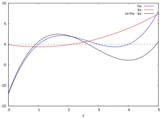
4.2.2 Intersection Points of Two Polynomials Where do the two curves h(x) = x3

−8x2 + 19x −12 and k(x) = 1₂x2 − x− 1₈ intersect? We want

approximate numerical values. We can plot the two functions together and use the cursor to read off the values of x for which the curves cross, and we can also nd the roots numerically. We rst dene the curves as expressions depending on x, then dene the difference of the expressions (rx) to work with using allroots rst to see if all the (three) roots are real, and then using realroots just for fun, and then checking the solutions. If we are just going to compare the results with a plot, we don't need any great accuracy, so we will use the default realroots precision.

(%i1) fpprintprec : 8$

(%i2) hx : x3 - 8*x2 + 19*x - 12$ (%i3) kx : x2/2 -x -1/8$

(%i4) rx : hx - kx;

2

3 17 x 95

(%o4) x - - + 20 x -

(19)

(%i5) factor(rx);

3 2

8 x - 68 x + 160 x - 95

(%o5)

---8 (%i6) define( fr(x), rx )$

(%i7) allroots(rx);

(%o7) [x = 0.904363, x = 2.6608754, x = 4.9347613]

(%i8) rr : float( realroots(rx) );

(%o8) [x = 0.904363, x = 2.6608754, x = 4.9347613]

(%i9) rr : map( rhs, rr);

(%o9) [0.904363, 2.6608754, 4.9347613]

(%i10) map(fr, rr);

(%o10) [2.04101367E-8, - 8.4406409E-8, 5.30320676E-8]

We see that the numerical solutions are zeros of the cubic function to within the numerical accuracy realroots is using. Just out of curiosity, what about exact solutions of this cubic polynomial? Use of solve will generate a complicated looking expression involving roots and %i. Let's set display2d to false so the output doesn't take up so much room on the screen.

(%i11) display2d : false$ (%i12) sx : solve(rx);

(%o12) [x = (-sqrt(3)*%i/2-1/2)*(3-(3/2)*sqrt(16585)*%i/16+151/432)(1/3) +49*(sqrt(3)*%i/2-1/2)/(36*(3-(3/2)*sqrt(16585)*%i/16+151/432)

(1/3))+17/6, etc, etc ]

(%i13) sx1 : map(rhs, sx);

(%o13) [(-sqrt(3)*%i/2-1/2)*(3-(3/2)*sqrt(16585)*%i/16+151/432)(1/3) +49*(sqrt(3)*%i/2-1/2)/(36*(3-(3/2)*sqrt(16585)*%i/16+151/432)

(1/3))+17/6, etc, etc ]

The list sx1 holds the exact roots of the cubic polynomial which solve found. We see that the form returned has explicit factors of %i. We already know that the roots of this polynomial are purely real. How can we get the exact roots into a form where it is obvious that the roots are real? The Maxima expert Alexey Beshenov (via the Maxima mailing list) suggested using rectform, followed by trigsimp. Using rectform gets rid of the factors of %i, and trigsimp does some trig simplication.

(%i14) sx2 : rectform(sx1);

(%o14) [49*(3*sqrt(3)*sin(atan(432*3-(3/2)*sqrt(16585)/(151*16))/3)/7 -3*cos(atan(432*3-(3/2)*sqrt(16585)/(151*16))/3)/7)/36

+7*sqrt(3)*sin(atan(432*3-(3/2)*sqrt(16585)/(151*16))/3)/12 +%i*(-7*sin(atan(432*3-(3/2)*sqrt(16585)/(151*16))/3)/12 +49*(3*sin(atan(432*3-(3/2)*sqrt(16585)/(151*16))/3)/7

+3*sqrt(3)*cos(atan(432*3-(3/2)*sqrt(16585)/(151*16))/3)/7)/36 -7*sqrt(3)*cos(atan(432*3-(3/2)*sqrt(16585)/(151*16))/3)/12)

-7*cos(atan(432*3-(3/2)*sqrt(16585)/(151*16))/3)/12+17/6,

etc,etc ]

(%i15) sx3 : trigsimp(sx2);

(%o15) [ (7*sqrt(3)*sin(atan(9*sqrt(16585)/(151*sqrt(3)))/3) -7*cos(atan(9*sqrt(16585)/(151*sqrt(3)))/3)+17)/6, -(7*sqrt(3)*sin(atan(9*sqrt(16585)/(151*sqrt(3)))/3)

(20)

The quantity sx3 is a list of the simplied exact roots of the cubic. Using oat we ask for the numerical values:

(%i16) sx4 : float(sx3);

(%o16) [2.6608754,0.904363,4.9347613]

We see that the numerical values agree, although the order of the roots is different. Next we enquire whether or not the exact roots, when substituted back into the cubic, result in exact zeroes. Mapping the cubic onto the list of roots doesn't automatically simplify to a list of three zeroes, as we would like, although applying oat suggests the analytic roots are correct. The combination

trigsimp( expand( [fr(root1), fr(root2), fr(root3)] ) ) still does not provide the alge-braic and trig simplication needed, but we nally get [0.0, 0.0, 0.0] when applying oat.

(%i17) float( map(fr, sx3) );

(%o17) [-3.55271368E-15,1.88737914E-15,-1.42108547E-14] (%i18) float( expand( map(fr, sx3) ) );

(%o18) [6.66133815E-16,-2.44249065E-15,0.0]

(%i19) float( trigsimp( expand( map(fr, sx3) ) ) ); (%o19) [0.0,0.0,0.0]

Let's next plot the three functions, using the expressions hx, kx, and rx (the difference).

-15 -10 -5 0 5 10

0 1 2 3 4 5

x

hx kx rx=hx - kx

Figure 2: Intersection Points are Zeroes of rx

Here is code you can use to make something close to the above plot.

(%i20) plot2d([hx,kx,rx],[x,0,5],

[style, [lines,2,1], [lines,2,2], [lines,2,0] ], [legend, "hx", "kx", "rx=hx - rx"],

[gnuplot_preamble, " set xzeroaxis lw 2 "])$

(21)

4.2.3 Transcendental Equations and Roots: nd root

A transcendental equation is an equation containing a transcendental function. Examples of such equations are x=ex _and_x _{= sin(}_x₎_{. The logarithm and the exponential function are examples of transcendental functions.} We will include the trigonometric functions, i.e., sine, cosine, tangent, cotangent, secant, and cosecant in this category of functions. (A function which is not transcendental is said to be algebraic. Examples of algebraic functions are rational functions and the square root function.)

To nd the roots of transcendental expressions, for example, we can rst make a plot of the expression, and then use nd root knowing roughly where nd root should start looking. The Maxima manual provides a lot of details, beginning with:

Function: nd root(expr, x, a, b) Function: nd root(f, a, b)

Option variable: nd root error Option variable: nd root abs Option variable: nd root rel

Finds a root of the expression expr or the function f over the closed interval [a, b]. The expression expr may be an equation, in which case find_root seeks a root of lhs(expr) - rhs(expr). Given that Maxima can evaluate expr or f over [a, b] and that expr or f is continuous, find_root is guaranteed to nd the root, or one of the roots if there is more than one.

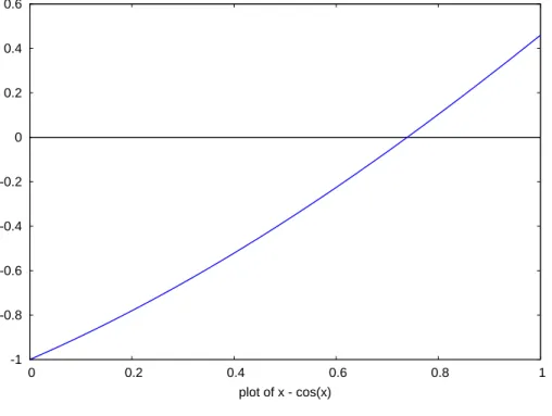
Let's nd a root of the equationx= cos(x). If we make a simple plot of the functionx−cos(x), we see that

there is one root somewhere betweenx= 0andx= 1.

-1 -0.8 -0.6 -0.4 -0.2 0 0.2 0.4 0.6

0 0.2 0.4 0.6 0.8 1

plot of x - cos(x)

Figure 3: Plot of x - cos(x)

(22)

We can make a plot, nd the root in a variety of ways using nd root, and verify the accuracy of the root as follows:

(%i2) plot2d( x - cos(x), [ x, 0, 1 ], [style, [lines, 4, 1] ],

[xlabel," plot of x - cos(x) "],

[gnuplot_preamble, "set nokey; set xzeroaxis lw 2 "] )$ (%i3) find_root( x - cos(x),x, 0, 1);

(%o3) 0.739085

(%i4) ex : x - cos(x)$

(%i5) [find_root( ex, x, 0, 1),find_root( ex, 0, 1)];

(%o5) [0.739085, 0.739085]

(%i7) [find_root(f(x), x, 0, 1), find_root(f(x), 0, 1), find_root(f, 0, 1), find_root(f, x, 0, 1)];

(%o7) [0.739085, 0.739085, 0.739085, 0.739085]

(%i8) ev(ex, x = first(%) );

(%o8) 0.0

As a second example, we will nd the roots of the function

f(x) = cos(x/π)e−(x/4)2

−sin(x3/2)−5/4

Here is the plot off(x).

-2.5 -2 -1.5 -1 -0.5 0 0.5

0 1 2 3 4 5

plot of f(x)

Figure 4: Plot of f(x)

(23)

Here is our session making a plot and using nd root:

(%i2) f(x):= cos(x/%pi)*exp(-(x/4)2) - sin(x(3/2)) - 5/4$

(%i3) plot2d( f(x),[x,0,5],

[style, [lines,4,1] ],

[xlabel," plot of f(x) "],[ylabel," "],

[gnuplot_preamble, "set nokey; set xzeroaxis lw 2 "] )$ (%i4) [find_root(f,2.5,2.6), find_root(f, x, 2.5, 2.6),

find_root(f(x),x,2.5,2.6), find_root(f(y),y,2.5,2.6)];

(%o4) [2.5410501, 2.5410501, 2.5410501, 2.5410501]

(%i5) [x1 : find_root(f,2.5,2.6),x2 : find_root(f, 2.9, 3.0 )];

(%o5) [2.5410501, 2.9746034]

(%i6) float( map(f, [x1,x2] ) );

(%o6) [3.33066907E-16, 2.77555756E-16]

We see that the numerical accuracy of nd root using default behavior is the normal accuracy of Maxima arithmetic.

4.2.4 nd root: Quote that Function!

The Maxima function nd root is an unusual function. The source code which governs the behavior of nd root has been purposely designed to allow uses like the following:

(%i2) find_root(diff(cos(2*x)*sin(3*x)/(1+x2),x), x, 0, 0.5);

(%o2) 0.321455

nd root evaluates the derivative and parks the resulting expression in the code function fr(x),say, to be used to probe where the function changes sign, as the code executes a bisection search for a root in the range called for. The code rst checks that the sign of the function fr(x) has opposite signs at the end points of the given range. Next the code makes small steps in one direction, checking at each step if a sign change has occurred. As soon as a sign change has occurred, the code backs up one step, cuts the size of the step in half, say, and starts stepping again, looking for that sign change again. This is a brute force method which will nd that root if there is one in the given interval. Of course the user can always evaluate the derivative and submit the resulting expression to nd root to nd the same answer, as in:

(%i3) ex : trigsimp( diff(cos(2*x)*sin(3*x)/(1+x2),x) ); 2

(%o3) - (((2 x + 2) sin(2 x) + 2 x cos(2 x)) sin(3 x)

2 4 2

+ (- 3 x - 3) cos(2 x) cos(3 x))/(x + 2 x + 1) (%i4) plot2d([0.0,ex],[x,-3,3])$

(%i5) find_root(ex,x,0,0.5);

(24)

If we assign the delayed derivative to an expression ex1, we can then use an argument ev(ex1,diff) to nd root as in:

(%i6) ex1 : 'diff(cos(2*x)*sin(3*x)/(1+x2),x); d cos(2 x) sin(3 x)

(%o6) -- (---)

dx 2

x + 1 (%i7) find_root(ev(ex1,diff),x,0,0.5);

(%o7) 0.321455

If we assign the delayed derivative to a function g(x), and assign ev(g(x),diff) to another function k(x), we can use nd root as in:

(%i8) g(x) := 'diff(cos(2*x)*sin(3*x)/(1+x2),x); d cos(2 x) sin(3 x)

(%o8) g(x) := -- (---)

dx 2

1 + x (%i9) k(x) := ev(g(x),diff);

(%o9) k(x) := ev(g(x), diff)

(%i10) find_root(k(x),x,0,0.5);

(%o10) 0.321455

or just use the syntax:

(%i11) find_root( ev(g(x),diff),x,0,0.5 );

(%o11) 0.321455

However, the following syntax which leaves out the variable name produces an error message:

(%i12) find_root( k, 0, 0.5 ); Non-variable 2nd argument to diff: 0.0

#0: g(x=0.0) #1: k(x=0.0)

In the above cases we want nd root to use the default initial evaluation of the rst slot argument before going to work looking for the root.

The important thing to stress is that the nd root source code, by default, is designed to evaluate the rst slot expression before beginning the checking of the sign of the resulting function (after evaluation) at the end points and proceeding with the bisection search. If the user wants to use (for some reason) a function f(x) in the rst slot of nd root and wishes to prevent the initial evaluation of the rst slot expression, the user should use the syntax '(f(x)) for the rst slot entry, rather than f(x). However, the code is loosely written so that most of the time you can get correct results without using the single quote syntax '(f(x)). All of the following examples give the correct answer for this simple function.

(%i13) f(x) := x - cos(x)$

(%i14) [find_root( f, 0, 1), find_root( 'f, 0, 1),

find_root( '(f), 0, 1), find_root( f(x), x, 0, 1),

find_root( '( f(x)), 'x, 0, 1),find_root( '( f(x)), x, 0, 1), find_root( 'f(x), x, 0, 1)];

(25)

However, one can arrive at specialized homemade functions which require the strict syntax (a quoted func-tion entry in the rst slot) to behave correctly. Suppose we need to nd the numerical roots of a funcfunc-tion dened by an integral. The following is a toy model which uses such a function in a case where we know the answer ahead of time. Instead of directly looking for the roots of the functionf(x) = (x2

−5), we look for the roots

of the functionRx √

52y d y.

(%i1) fpprintprec : 8$

(%i2) ex : integrate(2*'y,'y,sqrt(5),x); 2

x 5

(%o2) 2 (-- - -)

2 2

(%i3) ex : expand(ex);

2

(%o3) x - 5

(%i4) define( f(x), ex );

2

(%o4) f(x) := x - 5

(%i5) solve( ex );

(%o5) [x = - sqrt(5), x = sqrt(5)]

(%i6) rr : float( map(rhs,%) );

(%o6) [- 2.236068, 2.236068]

(%i7) map(f,rr);

(%o7) [8.8817842E-16, 8.8817842E-16]

(%i8) find_root(f,0,4);

(%o8) 2.236068

Let's concentrate on nding the root 2.23606797749979 using the indirect route. Dene a functiong(x)

in terms of integrate:

(%i9) g(x) := block([numer,keepfloat,y], numer:true,keepfloat:true, integrate(2*y,y,sqrt(5),x) )$ (%i10) map(g, [1,2,3]);

(%o10) [- 4.0, - 1.0, 4.0]

(%i11) map(f, [1,2,3]);

(%o11) [- 4, - 1, 4]

(%i12) [find_root( g, 1, 4), find_root( g(x),x,1,4),

find_root( '(g(x)),'x,1,4 ), find_root( 'g(x),x,1,4 )];

(%o12) [2.236068, 2.236068, 2.236068, 2.236068]

We see that we have no problems with getting the function g(x) to work with nd root. However, if

we replace integrate with quad qags, we nd problems. First let's show the numerical integration routine quad qags at work by itself:

(%i13) quad_qags(2*'y,'y,sqrt(5),2);

(%o13) [- 1.0, 1.11076513E-14, 21, 0]

(%i14) g(2.0);

(%o14) - 1.0

(26)

Here we dene h(x) which employs the function quad qags to carry out the numerical itegration.

(%i15) h(x) := block([numer,keepfloat,y,qlist], numer:true,keepfloat:true,

qlist : quad_qags(2*y,y,sqrt(5),x), qlist[1] )$

(%i16) map(h,[1,2,3]);

(%o16) [- 4.0, - 1.0, 4.0]

(%i17) map(g,[1,2,3]);

(%o17) [- 4.0, - 1.0, 4.0]

The functionh(x)does the same job asg(x), but uses quad qags instead of integrate. Now let's useh(x)in

the Maxima function nd root.

(%i18) find_root( h(x),x,1,4); function has same sign at endpoints [f(1.0) = - 5.0, f(4.0) = - 5.0]

We see that the syntax find_root( h(x),x,1,4) produced an error due to the way nd root evaluates the rst slot. Somehow nd root assigned -5.0 to the internal function fr(x) used to look for the root, and in the rst steps of that root location, checking for a difference in sign of fr(x) and the range end points, found the value -5.0 at both ends. In effect, the code was working on the problem find_root( -5.0, x, 1, 4).

The following methods succeed.

(%i19) [find_root( h, 1, 4),find_root( '(h(x)),'x,1,4 ), find_root( '(h(x)),x,1,4 ),find_root( 'h(x),x,1,4 )];

(%o19) [2.236068, 2.236068, 2.236068, 2.236068]

4.2.5 newton

The Maxima function newton can also be used for numerical solutions of a single equation. The Maxima manual describes the syntax as:

Function: newton(expr, x, x_0, eps)

Returns an approximate solution of expr = 0 by Newton's method, considering expr to be a function of one variable, x. The search begins with x = x_0 and proceeds until abs(expr) < eps (with expr evaluated at the current value of x).

newton allows undened variables to appear in expr, so long as the termination test abs(expr) < eps evaluates to true or false. Thus it is not necessary that expr evaluate to a number.

load(newton1) loads this function.

The two examples in the manual are instructive:

(%i1) fpprintprec:8$ (%i2) load (newton1);

(%o2) C:/PROGRA1/MAXIMA3.0/share/maxima/5.14.0/share/numeric/newton1.mac (%i3) newton (cos (u), u, 1, 1/100);

(%o3) 1.5706753

(%i4) ev (cos (u), u = %);

(%o4) 1.21049633E-4

(%i5) assume (a > 0);

(27)

(%i6) newton (x2 - a2, x, a/2, a2/100);

(%o6) 1.0003049 a

(%i7) ev (x2 - a2, x = %);

2

(%o7) 6.09849048E-4 a

Of course both of these examples are found exactly by solve:

(%i8) solve( cos(x) );

%pi

(%o8) [x = ---]

2 (%i9) float(%);

(%o9) [x = 1.5707963]

(%i10) solve( x2 - a2,x );

(%o10) [x = - a, x = a]

I nd the source code (Windows XP) in the folder

c:\Program Files\Maxima-5.14.0\share\maxima\5.14.0\share\numeric. Here is the code in the le newton1.mac:

newton(exp,var,x0,eps):= block([xn,s,numer],

numer:true, s:diff(exp,var), xn:x0,

loop,

if abs(subst(xn,var,exp))<eps then return(xn), xn:xn-subst(xn,var,exp)/subst(xn,var,s),

go(loop) )$

We see that the code implements the Newton-Raphson algorithm. Given a functionf(x)and an initial guess

xg which can be assigned to, say,xi, a closer approximation to the value ofxfor whichf(x) = 0is generated by

xi+1 =xi− f(x

i₎ f′₍_xi₎.

The method depends on being able to evaluate the derivative off(x)which appears in the denominator.

Steven Koonin's (edited) comments (Computational Physics: Fortran Version, Steven E. Koonin and Dawn Meredith, WestView Press, 1998, Ch. 1, Sec.3) are cautionary:

When the functionf(x)is badly behaved near its root (e.g., there is an inection point near the root) or when

(28)

4.3 Two or More Equations: Symbolic and Numerical Solutions

For sets of equations, we can use solve with the syntax:

Function: solve([eqn_1, ..., eqn_n], [x_1, ..., x_n])

solve ([eqn_1, ..., eqn_n], [x_1, ..., x_n]) solves a system of simultaneous (linear or non-linear) polynomial equations by calling linsolve or algsys and returns a list of the solution lists in the variables. In the case of linsolve this list would contain a single list of solutions. This form of solve takes two lists as arguments. The rst list represents the equations to be solved; the second list is a list of the unknowns to be determined. If the total number of variables in the equations is equal to the number of equations, the second argument-list may be omitted.

4.3.1 Numerical or Symbolic Linear Equations with solve or linsolve

The Maxima functions solve, linsolve, and linsolve by lu can be used for linear equations.

Linear equations containing symbolic coefcients can be solved by solve and linsolve. For example the pair of equations

ax+by =c, dx+ey=f

. Here we solve for the values of (x,y) which simultaneously satisfy these two equations and check the solutions.

(%i1) eqns : [a*x + b*y = c, d*x + e*y = f];

(%o1) [b y + a x = c, e y + d x = f]

(%i2) solve(eqns,[x,y]);

c e - b f c d - a f

(%o2) [[x = - ---, y = ---]]

b d - a e b d - a e

(%i3) soln : linsolve(eqns,[x,y]);

c e - b f c d - a f

(%o3) [x = - ---, y = ---]

b d - a e b d - a e

(%i4) (ev(eqns, soln), ratexpand(%%) );

(%o4) [c = c, f = f]

Note the presence of the determinant of the coefcient matrix in the denominator of the solutions.

A simple numerical (rather than symbolic) two equation example:

(%i1) eqns : [3*x-y=4,x+y=2];

(%o1) [3 x - y = 4, y + x = 2]

(%i2) solns : solve(eqns,[x,y]);

3 1

(%o2) [[x = -, y = -]]

2 2

(%i3) soln : solns[1];

3 1

(%o3) [x = -, y = -]

2 2

(%i4) for i thru 2 do disp( ev( eqns[i],soln ) )$ 4 = 4

(29)

Using linsolve instead returns a list, rather than a list of a list.

(%i5) linsolve(eqns,[x,y]);

3 1

(%o5) [x = -, y = -]

2 2

4.3.2 Matrix Methods for Linear Equation Sets: linsolve by lu

The present version (5.14) of the Maxima manual does not have an index entry for the function linsolve by lu. These notes include only the simplest of many interesting examples described in two mailing list responses by the creator of the linear algebra package, Barton Willis (Dept. of Mathematics, Univ. Nebraska at Kearney), dated Oct. 27, 2007 and Nov. 21, 2007.

If we re-cast the two equation problem we have just been solving in the form of a matrix equation

A . xcol = bcol, we need to construct the square matrix A so that matrix multiplication by the column vector xcol results in a column vector whose rows contain the left hand sides of the equations. The column vector bcol rows hold the right hand sides of the equations. Our notation below ( as xycol and xylist ) is only natural for a two equation problem (ie., a 2 x 2 matrix): you can invent your own notation to suit your problem.

If the argument of the function matrix is a simple list, the result is a row vector (a special case of a matrix object). We can then take the transpose of the row matrix to obtain a column matrix, such as xcol below. A direct denition of a two element column matrix is matrix([x],[y]), which is probably faster than transpose(matrix([x,y])). To reduce the amount of space taken up by the default matrix output, we can set display2d:false.

(%i6) m : matrix( [3,-1],[1,1] );

[ 3 - 1 ]

(%o6) [ ]

[ 1 1 ]

(%i7) display2d:false$ (%i8) m;

(%o8) matrix([3,-1],[1,1]) (%i9) xcol : matrix([x],[y]); (%o9) matrix([x],[y])

(%i10) m . xcol;

(%o10) matrix([3*x-y],[y+x])

The period allows non-commutative multiplication of matrices. The linear algebra package function lin-solve by lu allows us to specify the column vector bcol as a simple list:

(%i11) b : [4,2]; (%o11) [4,2]

(%i12) linsolve_by_lu(m,b);

(%o12) [matrix([3/2],[1/2]),false] (%i13) xycol : first(%);

(%o13) matrix([3/2],[1/2]) (%i14) m . xycol - b; (%o14) matrix([0],[0])

(%i15) xylist : makelist( xycol[i,1],i,1,length(xycol) ); (%o15) [3/2,1/2]

(30)

The matrix argument needs to be a square matrix. The output of linsolve by lu is a list: the rst element is the solution column vector which for this two dimensional problem we have called xycol.

We check the solution in input %i14. The output %o14 is a column vector each of whose elements is zero; such a column vector is ordinarily replaced by the number 0.

One should always check solutions when using computer algebra software, since the are occasional bugs in the algorithms used. The second list element returned by linsolve by lu is false, which should always be the value returned when the calculation uses non-oating point numbers as we have here. If oating point numbers are used, the second element should be either false or a lower bound to the matrix condition number. (We show an example later.) We have shown how to convert the returned xycol matrix object into an ordinary list, and how to then construct a list of replacement rules (as would be returned by linsolve) which could then be used for other purposes. The use of makelist is the recommended way to use parts of matrix objects in lists. However, here is a simple method which avoids makelist:

(%i17) flatten( args( xycol)); (%o17) [3/2,1/2]

but makelist should normally be the weapon of choice, since the method is foolproof and can be extended to many exotic ways of using the various elements of a matrix.

The Maxima function linsolve by lu allows the second argument to be either a list (as in the example above) or a column matrix, as we show here.

(%i18) bcol : matrix([4],[2])$ (%i19) linsolve_by_lu(m,bcol); (%o19) [matrix([3/2],[1/2]),false] (%i20) m . first(%) - bcol;

(%o20) matrix([0],[0])

4.3.3 Symbolic Linear Equation Solutions: Matrix Methods Here we use linsolve by lu for the pair of equations

ax+by=c, dx+ey=f,

seeking the values of (x,y) which simultaneously satisfy these two equations and checking the solutions.

(%i1) display2d:false$

(%i2) m : matrix( [a,b], [d,e] )$ (%i3) bcol : matrix( [c], [f] )$ (%i4) ls : linsolve_by_lu(m,bcol);

(%o4) [matrix([(c-b*(f-c*d/a)/(e-b*d/a))/a],[(f-c*d/a)/(e-b*d/a)]),false] (%i5) xycol : ratsimp( first(ls) );

(%o5) matrix([-(b*f-c*e)/(a*e-b*d)],[(a*f-c*d)/(a*e-b*d)]) (%i6) ( m . xycol - bcol, ratsimp(%%) );

(%o6) matrix([0],[0])

(%i7) (display2d:true,xycol);

[ b f - c e ]

[ - --- ]

[ a e - b d ]

(%o7) [ ]

[ a f - c d ] [ --- ] [ a e - b d ] (%i8) determinant(m);

(31)

We see the value of the determinant of the coefcient matrix m in the denominator of the solution.

4.3.4 Multiple Solutions from Multiple Right Hand Sides

Next we show how one can solve for multiple solutions (with one call to linsolve by lu) corresponding to a number of different right hand sides. We will turn back on the default matrix display, and re-dene the rst (right hand side) column vector as b1col, and the corresponding solution x1col.

(%i21) display2d:true$

(%i22) b1col : matrix( [4], [2] );

[ 4 ]

(%o22) [ ]

[ 2 ]

(%i23) x1col : first( linsolve_by_lu(m,b1col) ); [ 3 ]

[ - ] [ 2 ]

(%o23) [ ]

[ 1 ] [ - ] [ 2 ] (%i24) b2col : matrix( [3], [1] );

[ 3 ]

(%o24) [ ]

[ 1 ]

(%i25) x2col : first( linsolve_by_lu(m, b2col) ); [ 1 ]

(%o25) [ ]

[ 0 ] (%i26) bmat : matrix( [4,3], [2,1] );

[ 4 3 ]

(%o26) [ ]

[ 2 1 ] (%i27) linsolve_by_lu( m, bmat );

[ 3 ]

[ - 1 ]

[ 2 ]

(%o27) [[ ], false]

[ 1 ]

[ - 0 ]

[ 2 ]

(%i28) xsolns : first(%);

[ 3 ]

[ - 1 ]

[ 2 ]

(%o28) [ ]

[ 1 ]

[ - 0 ]

(32)

(%i29) m . xsolns - bmat;

[ 0 0 ]

(%o29) [ ]

[ 0 0 ] (%i30) x1col : col(xsolns,1);

[ 3 ] [ - ] [ 2 ]

(%o30) [ ]

[ 1 ] [ - ] [ 2 ] (%i31) x2col : col(xsolns,2);

[ 1 ]

(%o31) [ ]

[ 0 ]

In input %i26 we dene the 2 x 2 matrix bmat whose rst column is b1col and whose second column is b2col. Using bmat as the second argument to linsolve by lu results in a return list whose rst element (what we call xsolns) is a 2 x 2 matrix whose rst column is x1col (the solution vector corresponding to b1col) and whose second column is x2col (the solution vector corresonding to b2col). In input %i29 we check both solutions simultaneously. The result is a matrix with every element equal to zero, which would ordinarily be replaced by the number 0. In input %i30 we extract x1col using the col function.

4.3.5 Three Linear Equation Example

We next consider a simple three linear equation example. Although solve does not require the list [x,y,z] in this problem, if you leave it out, the solution list returned will be in an order determined by the peculiarities of the code, rather than by you. By including the variable list as [x,y,z], you are forcing the output list to be in the same order.

(%i1) eqns : [2*x - 3*y + 4*z = 2, 3*x - 2*y + z = 0, x + y - z = 1]$

(%i3) solns : solve( eqns,[x,y,z] ); (%o3) [[x = 7/10,y = 9/5,z = 3/2]] (%i4) soln : solns[1];

(%o4) [x = 7/10,y = 9/5,z = 3/2]

(%i5) for i thru 3 do disp( ev(eqns[i],soln) )$ 2 = 2

0 = 0 1 = 1

The Maxima function linsolve has the same syntax as solve (for a set of equations) but you cannot leave out the list of unknowns.

(%i6) linsolve(eqns,[x,y,z]); (%o6) [x = 7/10,y = 9/5,z = 3/2]

(33)

Next we use linsolve by lu on this three equation problem. Using the laws of matrix multiplication, we reverse engineer the3×3matrix m and the three element column vector bcol which provide an equivalent

problem in matrix form.

(%i7) m : matrix( [2,-3,4],[3,-2,1],[1,1,-1] )$ (%i8) xcol : matrix( [x],[y],[z] )$

(%i9) m . xcol;

(%o9) matrix([4*z-3*y+2*x],[z-2*y+3*x],[-z+y+x]) (%i10) bcol : matrix( [2],[0],[1] )$

(%i11) linsolve_by_lu(m,bcol);

(%o11) [matrix([7/10],[9/5],[3/2]),false] (%i12) xyzcol : first(%);

(%o12) matrix([7/10],[9/5],[3/2]) (%i13) m . xyzcol - bcol;

(%o13) matrix([0],[0],[0])

(%i14) xyzlist : makelist( xyzcol[i,1],i,1,length(xyzcol) ); (%o14) [7/10,9/5,3/2]

(%i15) xyzrules : map("=",[x,y,z],xyzlist); (%o15) [x = 7/10,y = 9/5,z = 3/2]

Both linsolve and solve can handle an equation list which is actually an expression list in which it is understood that the required equations are generated by setting each expression to zero.

(%i16) exs : [2*x - 3*y + 4*z - 2, 3*x - 2*y + z , x + y - z - 1];

(%o16) [4 z - 3 y + 2 x - 2, z - 2 y + 3 x, - z + y + x - 1]

(%i17) linsolve(exs,[x,y,z]);

7 9 3

(%o17) [x = --, y = -, z = -]

10 5 2

(%i18) solve(exs);

3 9 7

(%o18) [[z = -, y = -, x = --]]

2 5 10

The Maxima manual presents a linear equation example in which there is an undened parameter a.

(%i1) eqns : [x + z = y,2*a*x - y = 2*a2,y - 2*z = 2]$ (%i2) solns : linsolve(eqns,[x,y,z] );

(%o2) [x = a + 1, y = 2 a, z = a - 1]

(%i3) solve(eqns,[x,y,z]);

(%o3) [[x = a + 1, y = 2 a, z = a - 1]]

(%i4) for i thru 3 do (

e: expand( ev(eqns[i],solns) ),disp(lhs(e) - rhs(e)) )$ 0

0 0 (%i5) e;

(%o5) 2 = 2

(%i6) [kill(e),e];

(%o6) [done, e]

(34)

We can avoid introducing a global binding to a symbol by using %%, which allows use of the previous result inside a piece of code.

(%i7) for i thru 3 do (

expand( ev(eqns[i],solns) ),disp(lhs(%%) - rhs(%%)) )$ 0

0 0

Note the syntax used here: do ( job1, job2 ) .

Let's try out linsolve by lu on this three linear (in the unknowns (x,y,z)) equation problem which involves the unbound parameter a.

(%i9) m : matrix([1,-1,1],[2*a,-1,0],[0,1,-2] )$ (%i10) xcol : matrix( [x],[y],[z] )$

(%i11) m . xcol;

(%o11) matrix([z-y+x],[2*a*x-y],[y-2*z]) (%i12) bcol : matrix( [0],[2*a2], [2] )$ (%i13) soln : linsolve_by_lu(m,bcol)$

(%i14) xyzcol : ( first(soln), ratsimp(%%) ); (%o14) matrix([a+1],[2*a],[a-1])

(%i15) ratsimp( m . xyzcol - bcol); (%o15) matrix([0],[0],[0])

In input %i15 we check the solution, and the result is a three element column vector, all of whose elements are zero. Such a column matrix is ordinarily replaced by the number 0.

4.3.6 Surpressing rat Messages: ratprint

If we start with two linear equations with decimal coefcients, solve (and the other methods) converts the deci-mals to ratios of integers, and tries to nd an exact solution. You can avoid seeing all the rational replacements done by setting the option variable ratprint to false. Despite the assertion, in the manual section on rat, that

keepfloat if true prevents oating point numbers from being converted to rational numbers.

setting keepoat to true here does not stop solve from converting decimal numbers to ratios of integers.

(%i1) [keepfloat,ratprint];

(%o1) [false, true]

(%i2) display2d:false$ (%i3) fpprintprec:8$

(%i4) eqns : [0.2*x + 0.3*y = 3.3,0.1*x - 0.8*y = 6.6]$ (%i5) solns : solve(eqns, [x,y]);

`rat' replaced -3.3 by -33/10 = -3.3 `rat' replaced 0.2 by 1/5 = 0.2 `rat' replaced 0.3 by 3/10 = 0.3 `rat' replaced -6.6 by -33/5 = -6.6 `rat' replaced 0.1 by 1/10 = 0.1 `rat' replaced -0.8 by -4/5 = -0.8 (%o5) [[x = 462/19,y = -99/19]] (%i6) linsolve(eqns,[x,y]);

(35)

`rat' replaced 0.2 by 1/5 = 0.2 `rat' replaced 0.3 by 3/10 = 0.3 `rat' replaced -6.6 by -33/5 = -6.6 `rat' replaced 0.1 by 1/10 = 0.1 `rat' replaced -0.8 by -4/5 = -0.8 (%o6) [x = 462/19,y = -99/19]

(%i7) m : matrix([0.2,0.3],[0.1,-0.8] )$ (%i8) bcol : matrix( [3.3], [6.6] )$ (%i9) linsolve_by_lu(m,bcol);

`rat' replaced 0.2 by 1/5 = 0.2 `rat' replaced 0.2 by 1/5 = 0.2 `rat' replaced 0.2 by 1/5 = 0.2 `rat' replaced 0.95 by 19/20 = 0.95

(%o9) [matrix([24.315789],[-5.2105263]),false] (%i10) ratprint:false$

(%i11) solns : solve(eqns, [x,y]); (%o11) [[x = 462/19,y = -99/19]] (%i12) linsolve(eqns,[x,y]); (%o12) [x = 462/19,y = -99/19] (%i13) linsolve_by_lu(m,bcol);

(%o13) [matrix([24.315789],[-5.2105263]),false] (%i14) float(solns);

(%o14) [[x = 24.315789,y = -5.2105263]]

Matrix methods for sets of linear equations can be solved using IEEE double oats (as well as big oats) by including an optional method specication 'floatfield after the input column vector (or matrix of input column vectors).

(%i15) linsolve_by_lu(m,bcol, 'floatfield);

(%o15) [matrix([24.315789],[-5.2105263]),8.8815789]

In this example the lower bound of the matrix condition number appears as the second element of the returned list.

4.3.7 Non-Linear Polynomial Equations

Here is an example of using solve to nd a pair of exact solutions of a pair of equations, one equation being linear, the other quadratic. The pair of solutions represent the two intersections of the unit circle with the line y=−x/3.

(%i2) eqns : [x2 + y2 = 1, x + 3*y = 0]$ (%i3) solns : solve(eqns,[x,y]);

3 1

(%o3) [[x = - ---, y = ---],

sqrt(10) sqrt(2) sqrt(5)

3 1

[x = ---, y = - ---]]

(36)

(%i4) solns : rootscontract(solns);

3 1 3 1

(%o4) [[x = - ---, y = ---], [x = ---, y = - ---]]

sqrt(10) sqrt(10) sqrt(10) sqrt(10)

(%i5) for i thru 2 do for j thru 2 do (

ev(eqns[i],solns[j]), disp(lhs(%%)-rhs(%%)) )$ 0

0 0 0 (%i6) float(solns);

(%o6) [[x = - 0.948683, y = 0.316228], [x = 0.948683, y = - 0.316228]]

The pair of solutions reect the symmetry of the given set of equations, which remain invariant under the transformationx→ −y, y→ −x.

A set of two nonlinear polynomial equations with four solutions generated by solve is one of the examples in the Maxima manual. One of the solutions is exact, one is a real inexact solution, and the other two solutions are inexact complex solutions.

(%i2) eqns : [4*x2 - y2 = 12, x*y - x = 2]$ (%i3) solns : solve( eqns, [x,y] );

(%o3) [[x = 2, y = 2], [x = 0.520259 %i - 0.133124,

y = 0.0767838 - 3.6080032 %i], [x = - 0.520259 %i - 0.133124, y = 3.6080032 %i + 0.0767838], [x = - 1.7337518, y = - 0.153568]] (%i4) for i thru 2 do for j thru length(solns) do (

expand( ev(eqns[i],solns[j]) ),

abs( lhs(%%) - rhs(%%) ), disp(%%) )$ 0

2.36036653E-15 2.36036653E-15 1.13954405E-6

0 0.0 0.0 9.38499825E-8

(37)

4.3.8 General Sets of Nonlinear Equations: eliminate, mnewton

Solving systems of nonlinear equations is much more difcult than solving one nonlinear equation. A wider variety of behavior is possible: determining the existence and number of solutions or even a good starting guess is more complicated. There is no method which can guarantee convergence to the desired solution. The computing labor increases rapidly with the number of dimensions of the problem.

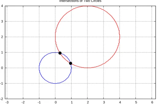
4.3.9 Intersections of Two Circles: implicit plot

Given two circles, we seek the intersections points. We rst write down the dening equations of the two circles, and look visually for points (x,y) which simultaneously lie on each circle. We use implicit plot for this visual search.

(%i1) [eq1 : x2 + y2 = 1,eq2 : (x-2)2 + (y-2)2 = 4]$ (%i2) eqns : [eq1,eq2]$

(%i3) load(implicit_plot); (%o3)

C:/PROGRA1/MAXIMA3.0/share/maxima/5.14.0/share/contrib/implicit_plot.lisp (%i4) implicit_plot(eqns,[x,-6,6],[y,-6,6],[nticks,200],

[gnuplot_preamble, "set zeroaxis" ])$

We are not taking enough care with the x and y ranges to make the circles circular, but we can use the cursor to read off approximate intersections points: (x,y) = (0.26,0.98), (0.96,0.30). However, the dening equations are invariant under the symmetry transformation x ↔ y, so the solution pairs must also

respect this symmetry. We next eliminate y between the two equations and use solve to nd accurate values for the x's. Since we know that both solutions have positive values for y, we enforce this condition on equation 1.

(%i5) solve(eq1,y);

2 2

(%o5) [y = - sqrt(1 - x ), y = sqrt(1 - x )]

(%i6) ysoln : second(%);

2

(%o6) y = sqrt(1 - x )

(%i7) eliminate(eqns,[y]);

2

(%o7) [32 x - 40 x + 9]

(%i8) xex : solve(first(%));

sqrt(7) - 5 sqrt(7) + 5

(%o8) [x = - ---, x = ---]

8 8

(%i9) (fpprintprec:8, xex : float(xex) );

(%o9) [x = 0.294281, x = 0.955719]

(%i10) [x1soln : first(xex), x2soln : second(xex) ]$ (%i11) [ev(%o7,x1soln), ev(%o7,x2soln)];

(%o11) [[- 4.4408921E-16], [0.0]]

(%i12) y1soln : ev(ysoln,x1soln);

(%o12) y = 0.955719

(%i13) y2soln : ev(ysoln,x2soln);

(%o13) y = 0.294281

(%i14) [soln1:[x1soln,y1soln],soln2:[x2soln,y2soln] ]$ (%i15) [ev(eqns,soln1), ev(eqns,soln2) ];

(%o15) [[1.0 = 1, 4.0 = 4], [1.0 = 1, 4.0 = 4]]

(%i16) [soln1,soln2];

(38)

We have solutions (%o16) which respect the symmetry of the equations. The solutions have been numerically checked in input %i15.

-2 -1 0 1 2 3 4

-3 -2 -1 0 1 2 3 4 5 6

Intersections of Two Circles

Figure 5: two circles

4.3.10 Using Draw for Implicit Plots

The gure above was created using the draw package with the following code in a separate work le implic-itplot1.mac. The code the the le is

/* file implicitplot1.mac */

/* need load(implicit_plot); to use this code */ disp(" doplot() ")$

doplot() := block([ x,y, eq1, eq2, y1:-2, y2:4,r, x1 ,x2 ], r : 1.56,

x1 : r*y1, x2 : r*y2,

eq1 : x2 + y2 = 1, eq2 : (x-2)2 + (y-2)2 = 4, draw2d(

grid = true,

line_type = solid, line_width = 3, color = blue,

implicit(eq1, x, x1,x2, y, y1,y2), color = red,

implicit(eq2, x, x1,x2, y, y1,y2), color = black,