#633 | 2020
Student segregation across and within
schools. The case of the Portuguese
public school system
JOÃO FIRMINO, LUÍS CATELA NUNES, SÍLVIA DE ALMEIDA,
SUSANA BATISTA
1
Student Segregation Across and Within Schools. The Case of the Portuguese Public
School System.
João Firmino
a,1,*; Luís Catela Nunes
a,2; Sílvia de Almeida
b,3; Susana Batista
c,4aNova School of Business and Economics, Universidade NOVA de Lisboa, Campus de Carcavelos, 2775-405 Carcavelos, Portugal bCICS.NOVA, Avenida de Berna, 26-C, 1069-061, Lisboa, Portugal
cInstituto Universitário de Lisboa (ISCTE-IUL), Centro de Investigação e Estudos de Sociologia, Lisboa, Portugal 1[email protected]; 2[email protected]; 3[email protected]; 4 [email protected]
* Corresponding author
Abstract
We provide the most comprehensive description of student segregation in the Portuguese public school system to date, a system that exhibits interesting institutional features potentially linked with the student segregation issue (e.g. school catchment areas, course tracking, and almost no central regulations regarding class composition). The analysis uses the entire regular student population enrolled in all public schools of continental Portugal (grades 1 to 12, from 2006/07 to 2016/17). Looking at three segregation dimensions – economic, academic, and immigrant – at both between and within-school levels, and using a novel dissimilarity index recently proposed in the literature aimed at better capturing systematic segregation, we find that segregation, on median, is mild, across time, grades, and regions. The most important exception is the case of within-school academic segregation. During upper-secondary schooling, in particular, when students are divided across classes according to own course-tracking decisions, it doubles. Moreover, within-school academic segregation estimates have the largest interquartile ranges, within a given year, grade, or region, pointing to heterogeneity in the way different schools set up classes internally in terms of students’ academic characteristics. Academic and economic segregation are positively associated, at both between and within school levels. The Portuguese segregation insights are also compared to those from other geographies.
Keywords: segregation; dissimilarity index; municipalities; schools; classes
2
1
Introduction
Contemporaneous societies value knowing how students seat across schools and, within schools, across classes. The accumulated evidence on cognitive and non-cognitive peer effects strongly supports this view (Sacerdote, 2011). Year after year students and parents decide, to some extent, on which school to attend and on which class to bargain for, partly based on those effects (known or perceived). Teachers are also likely pursuing a seat on specific schools and classes partly conditional on actual or expected student composition (Horng, 2009). On the other hand, knowledge on the distribution of students across and within schools is important to understand what kind of student sorting policies are being implemented by schools and by the relevant local or central governments (West & Wöβmann, 2006; Bloom, Lemos, Sadun &Van Reenen, 2015). Such policies must be checked to determine if they conform with societal values related to equity and social inclusion or not, or whether students’ quality of education, in particular, and quality of life, in general, might be at risk or not under them. It is then key to supply coherent and extensive measures of student segregation, that is, of how they are unevenly sorted, both across and within schools, so that all major actors of the education system can act upon, and the society in general judge upon, on the actual, real, distribution of students.
Portugal, the country here analyzed, is not an exception to these considerations. The objective of this article is to precisely describe the state of student segregation in Portugal. In doing so, the following research questions will be our focus. Does between and within-school segregation vary over time, grades, and districts? Do between and within-school segregation levels differ from one another? What is the relationship between minority shares and segregation levels, and between different dimensions of segregation? We believe this study provides the answers to these research questions and is able to match them with institutional features of the Portuguese school system.
The empirical analysis uses the dataset compiled by the Sistema de Informação do Ministério da Educação1
(MISI). This student-level administrative database follows all students, from all twelve grades, enrolled in public (state-owned, state-managed) schools in continental Portugal, throughout an entire decade (2006/07 – 2016/17). Given information on the actual classes and schools students were placed in, and on the schools’ location (namely the municipality where they are located), we are able to analyze student segregation at two distinct levels: between-schools (within-municipality), and within-between-schools (across classes of the same grade). For each of these levels we look at three segregation dimensions, each stemming from specific students’ dichotomous characteristics: economic (low-income vs non-low-income), academic (at least one retention vs no retentions), and immigrant (born abroad or with at least one parent born abroad vs all three not born abroad). Segregation is measured with the density-corrected
dissimilarity index (Ddc) recently proposed by Allen, Burgess, Davidson, & Windmeijer (2015) to capture systematic
segregation more robustly than the classic dissimilarity index (D).
Our main findings are that (1) there is a substantial increase in within-school academic segregation (and just a modest one for within-school economic segregation), during upper-secondary as compared to previous grades; (2) between-school segregation varies somewhat across primary, upper-primary, lower-secondary, and upper-secondary, but much less across grades within each of these stages; (3) over time, all segregation dimensions, at both between and within-school levels, exhibit time-invariant mild levels, with the case of within-school academic segregation presenting the highest values; (4) regional differences are more marked in terms of between-school segregation rather
3 than within-school, with the municipalities belonging to the districts of Lisboa and Setúbal (the country’s capital area) exhibiting the relative highest (and most precisely estimated) levels of unevenness in the way students are placed across schools; and (5) there is a mild positive association between academic and economic segregation, at both between and within-school levels (after netting-out several confounding factors). These are important findings as they indicate that academic, and to a lesser extent economic, characteristics of the students correlate with their observed placement, both between and within schools. Immigrant status of students also correlates with their placement, but this dimension does not seem to present higher segregation levels than the other two dimensions analyzed.
We show that certain characteristics of the Portuguese public education system seem to explain (up to a certain degree) the patterns found. Namely, (1) the upper-secondary tracking regime for the differing segregation levels before and after grade 10; (2) the differing granularities of the networks of primary, upper-primary, and lower and upper-secondary schools combined with the existence of school-catchment areas for the differences in between-school segregation levels across those educational stages (and districts); and (3) the vagueness of central regulations regarding class composition for within-school segregation patterns in general.
Domestic and international researchers and analysts will value this paper for the following three contributions. First, it offers a comprehensive and coherent study of the student segregation phenomena across what seem to be the main dimensions and levels of analysis usually adopted in the school segregation literature (economic, academic, immigrant; between and within schools), for the same country and period. To our knowledge, this is rare in the literature with past studies more often providing analyses restricted to fewer combinations of dimensions/levels of segregation. Although quite likely due to perfectly legitimate reasons such as researchers’ own research interests or limited data availability, the apparent scarcity of studies offering a more overarching type of analysis, such as the one we present here forces any interested reader to compare evidence related to different kinds of segregation from different sources. Due to differences of regions, periods, and idiosyncratic data treatment procedures likely found across them, comparability may be less straightforward, something that we believe to be avoided in this work (Conger, 2005, is an interesting example of another comprehensive study of segregation in terms of offering both a between and within-school analysis, though merely dedicated to the immigrant/racial dimension, see Table 1).
Secondly, it uses almost the entire student population of a European country throughout more than a decade, which also is uncommon in the literature (Allen & Vignoles, 2007, is a similar example for England, 1989-2004, see Table 1). Lastly, the Portuguese public education system likely contains characteristics similar to those located in other geographies and economies, meaning that similar segregation patterns might be at work there (e.g. Mediterranean Region, and Latin America). The Portuguese case may then be a useful reference point.
The following Section reviews the literature related with three important topics for this study: (1) the broad peer effects, (2) the methodology to measure segregation, and (3) studies on segregation or related subjects devoted to the Portuguese case and to that of other geographies to better highlight the contributions of this paper. Section 3 details the institutional context of the Portuguese education system, namely features related to the allocation process whereby students are placed across schools and classes. Section 4 presents the data. Section 5 discusses the actual methodology employed to measure segregation. The segregation estimates are provided in Section 6. Section 7 concludes.
4
2
Literature Review
One of the main reasons why student segregation is of concern has to do with the suspicion that similar students placed in schools or classes with different types of peers may lead those students to adopt different behaviors that otherwise they would not. Different behaviors are likely tied to different outcomes (educational or other) meaning that different segregation patterns are potentially linked to unequal educational or life opportunities.
In this regard, the economics of education peer effects literature has been gradually establishing the causal relationship between exposure to certain types of peers and individual students’ outcomes, Sacerdote (2011), though some uncertainties remain regarding magnitudes and non-linearities of the effects. Exposure to higher achieving peers, in particular, has been argued to be incremental to individual cognitive outcomes, especially for individuals in the bottom of the achievement distribution. On this, some interesting studies employing large administrative datasets (fixed effects estimations) are Hanushek, Kain, Markman & Rivkin (2003); Sund (2009); Lavy, Silva and Weinhardt (2012); Arcidiacono, Foster, Goodpaster & Kinsler (2012); and Burke and Sass (2013). The last two of these also present evidence that peer effects are more intense in specific disciplines (requiring more collaborative work) and at the class rather than at the school-grade level. Importantly, Burke and Sass (2013) demonstrate that the peers’ ability effect on individual performance is sensitive to the initial achievement level of the student in a non-monotone way (i.e. it is incremental to be exposed to academically gifted peers, but not with peers who are much more gifted relative to own baseline level). Applying instrumental variable strategies, Lefgren (2004) and De Giorgi, Pellizzari, & Woolston (2012) provide more evidence on peers’ ability positively impacting individual outcomes, though faintly, as well as on classroom ability heterogeneity (no heterogeneity meaning total segregation in academic ability) having an inverse U-shaped relationship with individual performance (thus suggesting the existence of an optimal strictly positive level of class ability heterogeneity). Contrasting with the De Giorgi et al. (2012) study, Duflo, Dupas, & Kremer (2011) offer experimental evidence supporting the view that increasing the percentage of top achieving
classmates positively influences all studentswithin the school. Meaning that sorting students across homogeneous
classes (according to previous academic achievement) would be the desirable policy.
The effects of racial peer composition on student achievement has also been examined, though more often in the context of USA schools. For example, Hoxby (2000); Angrist & Lang (2004); and Hanushek, Kain, & Rivkin (2009) find that peer effects are stronger intra-race and that larger shares of black students negatively affect black students, with no significant reciprocal effect on whites. Hoxby (2000) also deals with gender peer effects.
Looking at the Portuguese case, Firmino, Nunes, Reis, & Seabra (2018), find preliminary evidence that for Portuguese students (grades 5 through 9), too, there seem to exist important classroom peer effects, namely a negative impact from sharing the classroom with low-income students. In line with this, Seabra, Carvalho, & Ávila (2019)
also document a negative effect from exposure to larger concentrations of low SES students in Portugal (4th graders),
at the school-grade level, especially for African descendent students.
Some studies have examined peer effects beyond those related to pure academic achievement. Verkuyten & Thijs (2004) document a negative relationship between the class proportion of non-foreigners and foreigner students’ self-esteem, in the Netherlands. In the USA, analyzing the Moving to Opportunity program, which diminished economic segregation across neighborhoods by displacing low-income families to less impoverished zones in the cities, Ludwig, Duncan, Gennetian, Katz, et al. (2013) make the case that growing up in less impoverished
5 neighborhoods builds up subjective well-being, especially for low-income students, while Chetty, Hendren, & Katz (2016) document better long-term outcomes (higher chance for college enrollment, higher labor market earnings, and lower single parenthood rates) for sufficiently young moving children.
From the perspective of what might cause a non-random allocation of students, Bosworth (2014) interestingly documents empirical evidence supporting that classroom assignment is driven by students’ observables. Students’ characteristics are likely to be taken into account when it comes the time to decide on their distribution across classes, within any given school. Agents such as school authorities and parents likely try to optimally place them according to their specific preferences and goals, possibly to reap the benefits and avoid the costs from exposure to certain types of peers. Still on this topic, Levy & Razin (2017) present a theoretical model showing that due to a learning failure while in the labor market, repeating generations of parents may persist with different beliefs regarding which the best school might be (the most productivity-enhancing school) to send their children to, thus perpetuating segregation, even if there are no real differences between schools in terms of the value added accrued to students (i.e. to their offspring, the next generation of parents).
Turning to the topic of segregation measurement, several metrics have been proposed in the literature in past decades, see Frankel & Volij (2011) for a review. One sees at least three main sets of measures: group
interactions/exposure, diversity, and unevenness (OECD, 2019).2 Measuring group interactions relies on estimating
the likelihood that one member of one group comes into contact with members of (an)other group(s) (e.g. the exposure index, or its normalized version). Measuring diversity seeks to estimate how many different groups are represented within a given statistical unit, e.g. a school, see Reardon and Firebaugh (2002) and Frankel & Volij (2011) for recent theoretical and empirical applications on this. One possible example within this set of measures is the mutual information/entropy index. The third set of measures may be labeled as estimators of departures from evenness (with respect to the distribution of members belonging to one of two possible groups across statistical sub-units forming a wider unit, e.g. across classes within schools, or across schools within a geographical region).
Duncan & Duncan (1955) showed that many unevenness measures, for example the popular dissimilarity index (D) and the Gini coefficient (Gi), form a family of indexes related to the analysis of the segregation curve. Despite Massey & Denton (1988) claiming, based on factor and principal component analyses, that the dissimilarity index should be adopted as the reference within the set of unevenness measures, it too has been subject to criticism. Cortese, Falk, & Cohen (1976) noted that D uses as reference point the evenness scenario (𝐷 = 0), whereas researchers might be more interested to compare observed levels of segregation to the case of random allocation of individuals to units. Insofar as randomness in allocation generates expected strictly positive levels of unevenness (𝐷 > 0), it might be more informative to know by how much the observed distribution of individuals adds, in terms of unevenness, to that expectation and not to the eventual randomness-inconsistent case of complete evenness. Based on this insight, Carrington & Troske (1997) formulate another segregation index capable of measuring unevenness above (which would be seen as segregation) and, theoretically, also below (which would then be seen as inclusion) the expected level of unevenness consistent with randomness. On the other hand, the dissimilarity index has the virtue of not
2 Residential segregation literature conveys five types of measures: evenness, exposure, concentration, centralization, and
clustering (Massey & Denton, 1988). The last three types convey information regarding the spatial nature of segregation, which
6 depending mechanically on the minority share (at least under not too extremely small values of the minority share). This is convenient for comparisons of different statistical units with potentially different minority shares.
The Gorard index (G) (Gorard & Taylor, 2002) and the current concentration index (CC) (OECD, 2019) are
other possible measures of segregation that happen to be sensitive to the minority share.3 The Gorard index, in
particular, has been shown by Allen & Vignoles (2007) to not likely be the best choice (as compared with a segregation curve index such as D or Gi) to analyze segregation across schools given the potential large variations in minority shares across them (besides presenting other technical drawbacks such as not being 0-1 bounded, nor being symmetric). The square-root index is yet another segregation index proposed in Hutchens (2001) and Hutchens (2004). Although the square-root index satisfies seven important properties, the dissimilarity index satisfies five of these, failing only at two related with the ability to aggregate and with additive decomposability (see note 2 in Allen & Vignoles, 2007; we will elucidate these five properties of D in Section 5).
More recently, Allen et al. (2015) offer several correction procedures to the dissimilarity index in order to make it a measure of systematic segregation. The corrections aim to, precisely, partial-out the “bias” of strictly positive levels of unevenness that may be coherent with random allocation. These bias-adjustments are more intense whenever the fundamental parameters of unevenness segregation – minority share and unit sizes – are very small, which are the ones more likely to exacerbate D even under a random underlying allocation process. It is one of the bias-corrected dissimilarity indexes supplied in this last reference the one employed in this article to measure segregation, namely
their density-corrected dissimilarity index (Ddc).
As far as we are aware, there are no available analyses related to student segregation in Portugal, at least not comparable to the scope and magnitude of what we present here. Some studies look at specific types of students that are usually of interest to segregation analyses, such as those with immigrant background, e.g. Marques, Rosa, & Martins (2007), Hortas (2013), Roldão (2015), or those with specific ethnic background (e.g. Gypsy/Roma students, see Abrantes, Seabra, Caeiro, Almeida, & Costa, 2016; and Araújo, 2016). However, these do not delve into formal segregation analysis, but rely instead on describing socioeconomic contexts and their relationship to student achievement. Moreover, most of these studies employ methodologies such as the case-study or personal interviews that, in spite of offering a deep perspective on the few cases analyzed, fail to provide a comprehensive view of the
phenomena (i.e. they lack external validity).4 Central authorities have, to date and to the extent of our knowledge,
produced one study on student segregation: Baptista & Pereira (2018). However, this work merely analyzes
between-school economic segregation (within-districts; continental Portugal), only for 5th and 6th grade students (out of twelve
3 OECD (2019) provides the exact mathematical relationship among these indexes and the dissimilarity index: 𝐶𝐶 = 2𝑝𝐺 = 2𝑝(1 − 𝑝)𝐷, with CC, G, and D, as the indexes, and p as the minority share.
4 The Abrantes et al. (2016) and Araújo (2016) studies on Gypsy students are quite representative on this with the former focusing on one single public primary school in Lisboa, and the latter on another single public primary school in a rural area of Portugal. Nevertheless, they document extremely interesting insights. The former reports an outstanding 80% of the school population belonging to that single ethnic group, and with Gypsy parents reporting that they tend to be informally barred from enrolling their children in neighboring public primary schools. The latter documents a case of (total) white-flight from the school analyzed immediately after Gypsy parents started enrolling their children there. These constitute signs of strong ethnic between-school segregation (at least across primary schools) that, unfortunately, are impossible to extrapolate much further beyond those particular schools. Present Portuguese legislation prevents generalized collection of racial or ethnic information, which, understandably, forces researchers to apply case-study type of methodologies. Our dataset is not an exception. We are unable to study the between/within-school sorting of any ethnic/racial type of student. Hopefully, future versions of the database will provide more information regarding student ethnicity and/or race to allow fully understanding these phenomena and their real extent.
7 grades in total) and for the single 2015/16 school-year. Using a segregation measure describing the average difference between all possible pairs of schools (within a given district) in terms of proportion of low-income students, they find that schools situated in the most urban and populated districts such as Lisboa, Porto, and Setúbal (Map A1, Appendix A) exhibit the highest levels of economic segregation. In turn, Justino, Santos, Beatriz, Gramaxo et al. (2017) map a series of indicators related to students’ socioeconomic status, achievement levels, and teacher characteristics for all municipalities and schools of continental Portugal. Among their conclusions two relate closely with the analysis we present here: (1) immigrant students tend to be concentrated in municipalities/schools of the Lisboa metropolitan area and of Algarve (southernmost Faro district), and (2) they suggest that there is between-school economic segregation, especially in the most urban municipalities. Unfortunately, they do not provide formal segregation statistics. Finally, the interesting work of Bêa (2018) is, perhaps, the closest exercise that exists to ours. Bêa uses the same administrative database across the same school-years as we do, but looks only at between-school
segregation, just within the municipality of Lisboa, only across primary (1st cycle) schools, and uses the classic D.
Her main findings are that economic and immigrant between-school segregation levels in Lisboa seem to have been relatively high in the last decade. More specifically, Bêa estimates that around 40% of low-income and immigrant students would need to change from their current schools to another one in the city so that their distribution across Lisboa’s primary schools would be completely even.
Table 1 summarizes some of the empirical literature on student segregation since the early 2000s and compares several aspects with the present study. Despite not being an exhaustive list of all past studies on the topic we believe it suggests the Portuguese case we offer here expands the existing evidence in a number of aspects: (1) it is a non-Anglo-Saxon case encompassing the entire student population (grades 1 through 12) of a Southern European country; (2) it provides an overview of student segregation throughout a full recent decade; (3) it supplies a variety of combinations of different dimensions (economic, academic, and immigrant) and of distinct levels of analysis (between and within-school, the latter being the rarest in the related literature) of student segregation for the same education system, as well as a study on the structural correlations between all combinations of dimensions/levels of segregation and respective minority shares; and (4) uses the relatively recent density corrected dissimilarity index (Allen et al., 2015) as a more robust metric to measure segregation.
Finally, there are other important topics related to the student segregation topic in general that we should mention, though we will not delve into them here. One is that of quantifying the social welfare impact brought about by the uneven distribution of students across entities like schools or classes. We point to the Río & Alonso-Villar (2018) contribution as a clear methodological advance in this regard. The other is whether observed student segregation might be counteracted (or exacerbated) by students themselves. Holfve-Sabel (2015) presents the
interesting case of Swedish 6th graders who seem to offset, at least partially, within-school immigrant segregation
8 Tabl e 1 – Sa m p le o f Pap er s w it h E m p ir ica l R es u lt s on Stude n t Seg reg at ion Pa n el 1 G o ra rd & Ta y lo r (2 0 0 2 ) C o n g er (2 0 0 5 ) A ll en & V ig n o le s (2 0 0 7 ) F ra n k el & V o li j (2 0 1 1 ) B ar th o lo (2 0 1 3 ) A ll en e t al (2 0 1 5 ) G u ti ér re z et a l (2 0 1 7 ) B êa ( 2 0 1 8 ) M u ri ll o & M ar tí n ez -G ar ri d o (2 0 1 8) O EC D (2 0 1 9 ) P re sen t S tu d y S eg re g at io n I n d ex D ✓ ✓ ✓ 1 ✓ ✓ ✓ 4 ✓ ✓ D d c ✓ ✓ G ✓ ✓ ✓ S ( ex p o su re ) ✓ ✓ ✓ M I (mu tu al i n fo rm at io n ) ✓ 1 Le v el o f A n al y si s B et w ee n -sc h o o l w it h in -n at io n ✓ ✓ ✓ ✓ ✓ ✓ w it h in -st at e ✓ 2 ✓ w it h in -C B S A ✓ 2 w it h in -sc h o o l d ist ri ct ✓ ✓ 2 w it h in -mu n ic ip al it y ✓ ✓ ✓ w it h in -p ar ish ✓ w it h in -LEA ✓ ✓ W it h in -sc h o o l ac ro ss -c la sses ✓ ✓ D ime n si o n s o f S eg re g at io n S o ci o ec o n o m ic fr ee (o r re d u ce d p ri ce )-sc h o o l-mea l ✓ ✓ ✓ ✓ ✓ p ar en ts' e d u ca ti o n ✓ ✓ 6 b en ef ic ia ry o f p o v er ty a ll ev ia ti o n i n co me tr an sf er ✓ S ES ✓ 5 ✓ 5 ✓ 5 A ca d emi c ✓ ✓ Imm ig ra n t ✓ ✓ ✓ R ac ia l/ E th n ic ✓ ✓ ✓ C o rr el at io n A n al y si s amo n g se g re g at io n i n d ex es ( same se g re g at io n d im en si o n /l ev el o f an al y si s) ✓ ✓ ✓ 3 ✓ ✓ 3 amo n g se g re g at io n d im en si o n s ✓ ✓ amo n g se g re g at io n d im en si o n s an d m in o ri ti es ✓ Ty p e o f D at a A d mi n is tr at iv e d at as et ✓ ✓ ✓ ✓ ✓ ✓ ✓ ✓ LSI A ✓ ✓ ✓ 1al so A tk in so n , G in i, Ex p o su re , En tr o p y ; 2cr o ss -s ec ti o n a n al y si s o f 2 0 0 6 /0 7 ; 3imp li ci t; 4an d H u tc h en 's S q u ar e R o o t In d ex ; 5P IS A ESCS; 6al so r es id en ti al s eg re g at io n
9 Tabl e 1 – Sa m p le o f Pap er s w it h E m p ir ica l R es u lt s on Stude n t Seg reg at ion Pa n el 2 G o ra rd & Ta y lo r (2 0 0 2 ) C o n g er (2 0 0 5 ) A ll en & V ig n o le s (2 0 0 7 ) F ra n k el & V o li j (2 0 1 1 ) B ar th o lo (2 0 1 3 ) A ll en e t al (2 0 1 5 ) G u ti ér re z et a l (2 0 1 7 ) B êa ( 2 0 1 8 ) M u ri ll o & M ar tí n ez -G ar ri d o (2 0 1 8 ) O EC D ( 2 0 1 9 ) P re sen t S tu d y G ra d es P ri mary ✓ ✓ 1 ✓ ✓ ✓ 9 2 ✓ ✓ 9 3 ✓ ✓ 9 4 ✓ ✓ ✓ 9 U p p er -P ri mary ✓ 5 ✓ ✓ ✓ 6 ✓ Lo w er-S ec o n d ar y ✓ 7 ✓ 8 ✓ 9 ✓ ✓ ✓ ✓ U p p er -S ec o n d ar y ✓ ✓ ✓ 10 ✓ 11 ✓ 12 ✓ G eo g ra p h y UK ✓ ( W al es) ✓ ( En g la n d ) ✓ ( En g la n d -esp ec ia ll y in n er -L o n d o n LEA s) U S A ✓ ( N Y C sch o o l d is tr ic t) ✓ 7 P o rt u g al ✓ ( Li sb o a) ✓ B ra zi l ✓ ( R io d e Jan ei ro ) S p ai n ✓ 8 P IS A p ar ti ci p at in g c o u n tr ie s ✓ ✓ ( Eu ro p ea n U n io n co u n tr ie s) ✓ ( 7 1 co u n tr ie s/ re g i o n s) P er io d 1 9 8 9 -1 9 9 6 1 9 9 5 ; 2 0 0 0 1 9 8 9 -2 0 0 4 1 9 8 7 ; 2 0 0 7 2 0 0 4 -2 0 1 0 2 0 0 6 2 0 0 0 ; 2 0 0 3 ; 2 0 0 6 ; 2 0 0 9 ; 2 0 1 2 ; 2 0 1 5 2 0 0 7 -2 0 1 7 2 0 1 5 2 0 1 5 2 0 0 7 -2 0 1 7 N o te s: P er io ds se pa ra te d by ‘ -‘ me an s w ho le r an ge o f ye ar s w as an al yz ed ; s in gu la r ye ar s an al yz ed se pa ra te d by ‘ ;’ . 7p u b li c sc h o o ls o p er at in g a cr o ss s tu d ie d y ea rs ; 8w h o le c o u n tr y a n d a u to n o m o u s co mm u n it ie s; 9b et w ee n -sc h o o l se g re g at io n
10
3
Institutional Context
The Portuguese education system groups 12 sequential grades in four cycles across five main types of school
(Table A1, Appendix A).5 Pupils aged 5 (minority) or 6 (majority) years-old begin the 1st cycle at grade 1 and
complete it at the end of grade 4. Students enrolled in grades 6 and 9 finish the 2nd and 3rd cycles, respectively.
Upper-secondary – containing grades 10 to 12 – constitutes the final cycle of studies before labor market or college. The five types of school operating within the public system offer different combinations of cycles. Type-1
schools provide grades 1 to 4 and these grades can only be offered by such schools. Type-2 schools offer both 2nd
and 3rd cycles, spanning grades 5 to 9. Type-3 schools have students from cycles 2 to 4 (grades 5 to 12). Type-4
schools supply cycles 3 and 4, i.e. grades 7 to 12. Finally, type-5 schools offer only grades 10 to 12, i.e. only cycle 4.
Schools receive enrollment requests which they must then accept or reject according to criteria defined by the central government. When total enrollment requests to a given school are less than that school’s capacity there is no need to decide which students are allowed to enroll or not since the school has capacity to accept everyone. However, when demand for a school seat exceeds the school’s capacity an ordered list of criteria must then be followed to assess which applicants are given a place at the school. A simple summary of that list of criteria is as follows: (1) whether the student has a special education need, (2) whether the student was enrolled in that school in the previous year, (3) whether the student has a sibling enrolled in that school, (4) whether the student is recipient of socioeconomic support, (5) whether the student resides in the school catchment area, (6) whether a parent works in the school catchment area. This list of tie-breaks varies somewhat from cycle to cycle, and across school-years, with some criteria moving up or down one or two positions. In spite of possible variations of a criterion’s position, it shows that residential segregation may translate to between-school segregation given that residency impacts the school acceptance scheme both directly through criterion (5), as well as indirectly through criterion (4) as families tend to cluster in neighborhoods of relatively homogenous socioeconomic conditions (e.g. Malheiros & Vala, 2004 report clear spatial residential segregation patterns across parishes and neighborhoods belonging to the metropolitan area of Lisboa with respect to persons with a foreign nationality; this, in turn, may correlate with socioeconomic status).
Classes are usually maintained unchanged throughout all grades within a given cycle, by schools, hence school-induced segregation of students within-schools, across classes, should be more intensely observed at the beginning of each cycle (if any occurs). Especially if the beginning of the cycle coincides with moving to a new school. Specifically, these cases refer to students enrolling in grade 1 (always into a type-1 school), in grade 5 (always into type-2 or type-3 schools), in grade 7 (several possible school-move combinations between school types 2, 3, and 4), and in grade 10 (several possible school-move combinations between school types 2, 3, 4, and 5). There are two main exceptions: (i) students repeating a given grade who are displaced from their current class and reassigned to one of
5 From 2009/10 on, mandatory schooling was enlarged to encompass upper-secondary. Under this new regime, students are legally entitled to leave the education system (if they want so) only as soon as at least one of the following two conditions is true: (1) turning 18 years-old, or (2) having finished 12th grade. By contrast, the previous regime was mechanically the same, differing only in the thresholds: 15 years-old for condition (1), or completing 9th grade for condition (2). The new thresholds regime was enacted upon all students whom, by 2009/10 enrolled in 7th grade. By 2014/15 all students from all 12 grades were subject to the new regime. We should mention that although within the Portuguese public schooling system upper-secondary schooling is not formally called “4th cycle” (it is best known as secundário), we do so here for expositional simplicity.
11 the newly promoted classes of the grade they have to repeat (mixed-grade classes are only found in type-1 schools and for this reason we do not compute within-school segregation measures for grades 1 to 4; we come back to this issue when discussing the segregation measure used); and (ii) students moving from one school to another within a given cycle, or even within a given grade in the middle of a given academic year.
Whereas between-school sorting of students is clearly regulated whenever schools receive more enrollment requests than capacity, within-school (across classes) sorting of students, during the whole period considered, was quite vaguely regulated by the public authorities (see CNE, 2016 for a review on the evolution of legislation concerning class size and composition). In general, schools were mandated by law to translate each school-grade-year specific student heterogeneity across the respective classes, however with no concrete quantitative bounds on what it means to comply with that heterogeneity.
The Portuguese system contains a regular academic track and other tracks related to vocational education and other alternative educational paths. The regular track is by far the most demanded and we consider only these
students.6 Further, regular academic track students are required to choose one specific upper-secondary level course
when enrolling in grade 10 with the general options available being (1) exact sciences, (2) socio-economic sciences, (3) humanities/languages, and (4) arts/music (it may be the case that some schools may offer only a subset of these). Upper-secondary schools’ classes, in general, group students that opted for the same upper-secondary course.
Finally, it is important to mention that there have been changes during the period here considered in the way students can gain access to socioeconomic aid (which combine multiple discounts, such as reduced prices on school meals, transports, and textbooks). Whether students gained access to such discounts determines which ones we consider to belong to a low-income household. Although throughout the period analyzed the main philosophy behind the granting of the discounts has been constant – access conditional on sufficiently low per capita income at the household level – in 2008/09 there were two major changes (which were maintained until the last year of the dataset used). First, the determination of families’ income levels ceased to be done at the school level and became directly
linked to their family allowance category (determined by the central government).7 Second, the income thresholds to
accept a given family into one of the two major socioeconomic support levels, A and B, were relaxed. These two changes induced an increase in the proportion of students taking both levels, namely level A (the one we use as reference). We present the increase of the share of low-income students in the next Section, which details the dataset used.
6 Although we focus on segregation of students of the regular academic track across schools and across classes, we recognize that segregation of students across educational tracks is an interesting case for future analysis.
7 The formula to determine families’ income up to 2007/08 was regulated by the central government and thus common across them. However, the incumbency to check the veracity of each of the formula’s components (gross family income, health and housing expenditures, taxes and social security payments, and number of children) was on the local school side. The common perception, up to 2007/08, was that in the end this process gave schools the possibility to exert different levels of effort in checking the correctness of those figures, or that different schools with different administrative resources could act differently whenever doubts regarding the figures reported by families were raised. The 2008/09 reform was partly justified to make the process fairer to all families in the country in the sense that per capita income levels became determined by a central government procedure instead of being determined/confirmed at the local school level.
12
4
Data
The database used is MISI dataset, which is an administrative dataset collected by the Portuguese Ministry of Education. We use information on all students enrolled in public schools (in the regular academic track), in
continental Portugal8, from grades 1 to 12, and from 2006/07 to 2016/17. In other words, the majority of students
enrolled in the Portuguese public educational system throughout more than a decade. Table A2 (Appendix A) details the actual shares of students enrolled in the regular academic track and in public schools by cycle over time. In short, students enrolled in that track and, simultaneously, in public schools, comprise the large majority across cycles 1 through 3, and roughly half during upper-secondary (cycle 4). This information set is quite comprehensive, spanning, per year and on average (pooling all grades), around 1 million individual students, over about 5000 different schools, across all 278 municipalities of continental Portugal. Unlike earlier studies focused on the Portuguese case, external validity of our results should, in principle, not be an issue of concern (see discussion in Section 2).
Several students’ characteristics are available, as well as about their parents. In order to compute the measures of segregation we use information with respect to student and respective parents’ place of birth, whether the student belongs to a low-income household, and students’ age. From these characteristics we compute three dichotomous variables: low-income, at least one retention, and immigrant. Pupils with at least one retention are defined as those whose age is strictly greater than the maximum expected age at the beginning of the academic year (set to September
15th), making it an approximation to true retention. In turn, the maximum expected age is the maximum age the
student may be observed with, at the beginning of the academic year, given the current grade she is enrolled in, under
the scenario of not recording any retention since grade 1. These limiting ages start at 7 years old for 1st graders and
increment by one year of age for each grade, so, by the 12th grade, it is 18 years old. Note that these are exact ages,
so if a student is, say, 17.1 years old by September 15th and is enrolled in grade 11, then this student is given the
status of having at least one retention. Not doing so would imply that the student had entered grade 1 aged 7.1 years old, which is not permitted. As explained in the previous Section, students must enroll in grade 1 aged 6 years old
(or even 5 years old if they turn 6 between mid-September and December 31st), but not 7 or more.9 In turn, students
are given the status of belonging to a low-income household if they benefit from the most intense level of socioeconomic support at school (level A), the one allowing free school meals. The last dichotomous variable –
8 Students from the Atlantic islands’ autonomous regions of Azores and Madeira are not observed in the dataset.
9 The inconvenience of approximating true retention status via comparison of actual and (maximum) expected age is to erroneously not attribute such status to a group of students that, by grade g, possess, simultaneously, two characteristics: to only have been truly retained once between 1st grade and grade g, and, to have been enrolled in grade 1 aged strictly less than 6 years-old. The incidence of that error, however, is likely to be small. Note the following: (1) only around 29% of total students are born between 15th September and 31st December of any given year; (2) Madeira, Reis, Nunes, & Seabra (2018) state that, on average across school years, about 80% of students born between 15th September and 31st December enrol aged less than 6 years old (some parents opt to defer students’ entry age); and (3) Ikeda & García (2014) document, for Portugal, the actual retention rate is around 35% (percentage of 9th grade students reporting at least one retention – larger than the percentage of students with
exactly one retention, PISA 2009 data). Multiplying all three percentages shows that only about 7% of the students in our dataset
may have been given an erroneous retention status. Actually, the 7% figure is an upper bound of the true error incidence. As soon as some students of this particular group record a second, true, retention, then our approximation is again correct. On the bright side, our choice to not use true retentions, and instead an approximation, has the benefit that it is computable for all students. Even those that move from/to private schools or migrate. It does not rely on the ability to follow them over time, to then infer retention events by comparing grades in consecutive school-years within the student panel (which is not possible if within the student panel there are blanked school-years due to being enrolled in a school outside the continental Portugal public school system, e.g. a private school, or a school located in the Atlantic islands’ autonomous regions or in another country).
13
immigrant – attains value 1 if the student, or her mother, or her father, was not born in Portugal (if at least one of
these three persons has missing information regarding place of birth then it counts as a missing observation). The use of most of these dichotomous variables is not uncommon in school segregation analysis, and they are also endowed with some practical virtues. Proxying economic status via free school meal status seems the best alternative to us, as it has no missing observations, whereas other variables present in our dataset, such as parent education, parent job status, and parent occupation, do possess non-marginal amounts of missing information (there is no information on parent wage or actual household income). Allen & Vignoles (2007), Bartholo (2013), Allen et al. (2015), and Bêa (2018) use similar or exactly the same dichotomous variable to identify low-income students. Alternatively, Murillo, & Martínez-Garrido (2018) and OECD (2019) identify them as those below certain percentiles of the ESCS socioeconomic index distribution (PISA data). This alternative, however, is not suited for our setting as an equivalent socioeconomic index is not present in the dataset and computing it based on parental related variables would run into the missing information problem.
Identification of immigrant status of the student varies somewhat across studies, possibly depending on data availability on students’ (and parents’) nationalities and places of birth. For example, Bêa (2018) and Conger (2005) use only the students’ nationality and place of birth, respectively. Because we also possess information on parents’ place of birth we can identify as immigrants those also belonging to the second generation, which may well be subject to similar segregation pressures as first-generation immigrants.
The division between students with at least one retention from those recording none may be the least common way to distinguish low-achievers from other students. Alternatively, OECD (2019) categorizes as low-achievers those scoring in the bottom quartile of the PISA achievement distribution. Such a procedure in our setting is not impossible to implement as the dataset does possess students’ scores on national exams and on school-internal evaluations per subject. However, both sets of scores have serious drawbacks for our purposes in this study (besides also presenting non-marginal amounts of missing cases whenever such information is expected to exist). On one hand, the external scores are specific to certain grade/school-year combinations, which consequently precludes us from computing
segregation estimates for students enrolled in combinations with no external exams.10 On the other hand, the potential
lack of comparability of school internal marks across teacher–by–school–by–school-year combinations (internal marking is a subjective exercise likely to be driven by factors that differ across these cells) makes it a doubtful exercise to identify any given student as top or low-achiever in a definite way using such marks. Because this is a necessary step to compute segregation estimates, a clean interpretation of the latter would be jeopardized if one were to use the former scores. We thus view the distinction between students with (approximated) zero or at least one retention as a reasonable way to distinguish students with different educational outcomes (with that distinction being
reasonably coherent across school-years, grades, and places), while also implementable for the entire dataset.11
10 During the period of our dataset only 9th and 12th graders possess, for every school-year, external scores. Fourth and 6th graders have such scores only for a subset of all school-years. All remaining grades possess no external scores for the period covered. 11 We recognize that working with this variable has the drawback of not being able to compute academic segregation estimates for 1st graders, as these are not traditionally subject to retention. However, this is less restrictive than computing such estimates for 12th and 9th graders alone (and just some 4th and 6th graders’ cohorts). Such estimates should also be more coherent than academic segregation estimates based on internal scores, as different teachers may agree on an overall retention status more quickly than on specific marks for any particular student.
14 The MISI dataset also provides information on school and class membership for each student, as well as schools’
locations (district and municipality), for each academic year.12 This information enables us to compute the
segregation measures both between schools (within municipality) and within schools (across classes of the same grade).
Figures A1 through A5 in Appendix A decompose the three minorities’ shares over time, across grades, across
districts, across cycles over time, and across regions13 over time, respectively. In each Figure the first and
second-row graphs display the median shares of minorities taken from municipality-grade-year and school-grade-year
distributions, respectively.14 As remarked at the end of the previous section, the increase in the share of low-income
students is visible in the top left graphs of Figures A1 and A4. Around 5 p.p. comparing municipality-grade-year cases from 2008/09 with the two previous school-years in the former, and around 5 to 10 p.p. depending on the cycle for the latter. The bottom graphs of Figures A1 to A5 do not pool school-grade-year cases from grades 1 – 4 due to mixed-grade classes, and the medians thus do not take these into consideration; this explains why top and bottom graphs show slightly different patterns.
5
Methodology
As mentioned in the literature review, segregation has been measured through the dissimilarity index 𝐷𝑢𝑔𝑡:
𝐷𝑢𝑔𝑡 = 1 2∑ | 𝑚𝑖𝑛𝑜𝑟𝑖𝑡𝑦𝑠𝑔𝑡 𝑀𝑖𝑛𝑜𝑟𝑖𝑡𝑦𝑢𝑔𝑡 −𝑚𝑎𝑗𝑜𝑟𝑖𝑡𝑦𝑠𝑔𝑡 𝑀𝑎𝑗𝑜𝑟𝑖𝑡𝑦𝑢𝑔𝑡 | 𝑆𝑢𝑔𝑡 𝑠=1 =1 2∑|𝑝̂𝑠𝑔𝑡 1 − 𝑝̂ 𝑠𝑔𝑡0 | 𝑆𝑢𝑔𝑡 𝑠=1 (1)
for statistical unit u (statistical sub-units s nested within u), at grade g, and time period t. In our case, the statistical units will be the municipalities for the between-school segregation measures and the schools for the within-school
ones. The corresponding statistical sub-units will be the schools for the former, and the classes for the latter. 𝑆𝑢𝑔𝑡 is
the appropriate total number of schools (classes) observed in the municipality (school) u, in which there are students
of grade g, in period t. The index is then half of the summation (over all 𝑆𝑢𝑔𝑡 sub-units s of u) of the absolute
differences between the proportions of minority and majority students found in a given sub-unit s, 𝑝̂𝑠𝑔𝑡1 =
𝑚𝑖𝑛𝑜𝑟𝑖𝑡𝑦𝑠𝑔𝑡 𝑀𝑖𝑛𝑜𝑟𝑖𝑡𝑦𝑢𝑔𝑡
and 𝑝̂𝑠𝑔𝑡0 =
𝑚𝑎𝑗𝑜𝑟𝑖𝑡𝑦𝑠𝑔𝑡
𝑀𝑎𝑗𝑜𝑟𝑖𝑡𝑦𝑢𝑔𝑡, respectively. Note that these proportions measure the incidence of each group of students,
found in a given sub-unit, relative to each group size at the unit level, not the share of each type of student in that
sub-unit relative to the sub-unit’s size. Accordingly, 𝑚𝑖𝑛𝑜𝑟𝑖𝑡𝑦𝑠𝑔𝑡 (𝑚𝑎𝑗𝑜𝑟𝑖𝑡𝑦𝑠𝑔𝑡) is the number of minority (majority)
students found in sub-unit s, enrolled in grade g, in period t, while 𝑀𝑖𝑛𝑜𝑟𝑖𝑡𝑦𝑢𝑔𝑡 (𝑀𝑎𝑗𝑜𝑟𝑖𝑡𝑦𝑢𝑔𝑡) is the unit level
counterpart.
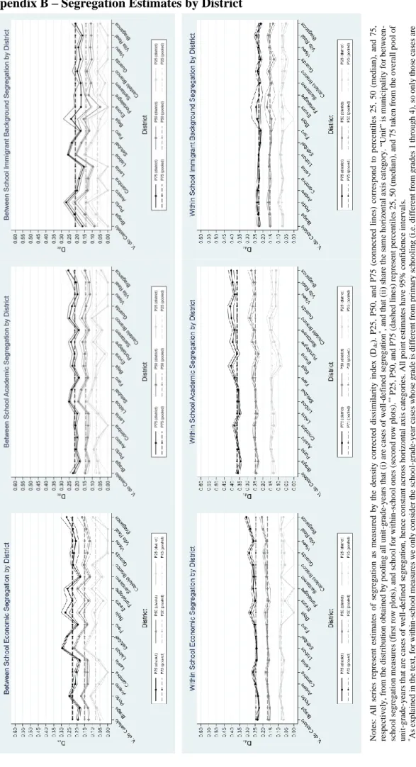
12 Continental Portugal is administratively divided into 18 districts, each containing several municipalities, see Map A1. 13 Whereas districts group municipalities, we define five regions grouping contiguous districts in order to simplify the exposition of some results over time. The assignment of districts to regions, although ad-hoc, is based on common knowledge regarding their social and demographic similarities (as well as on their geographical proximity). All minority shares (and all segregation measures presented in Section 6) are computed at the school or municipality level, but their estimates’ presentation is simplified (using the median) at the district or region level when assessing geographical patterns. Map A1 shows how districts were assigned to the five regions.
14 These distributions pool only cases of well-defined segregation for each relevant segregation dimension. Section 5 details what we consider a unit-grade-year to be a case of well-defined segregation.
15 The dissimilarity index is interpreted as the percentage of minority or majority students located in unit u (municipality or school), enrolled in grade g, in period t, who would have to change their current sub-unit (school or class) to achieve a completely even distribution.
As earlier studies point out, e.g. Carrington & Troske (1997) and Allen et al. (2015), the classic dissimilarity index expressed by equation (1) is a measure of segregation in the sense of accounting how unevenly students may be distributed across classes or schools, while not measuring the purposefulness of such distribution as the result of agents’ actions. Indeed, Allen et al. (2015) and Carrington & Troske (1997) show that usually some level of distributional unevenness is perfectly coherent with a random allocation process of individuals to sub-units. This is an important observation as we are interested in measuring systematic segregation in the sense of systematic deviations from whatever the level of unevenness that may be aligned with a random allocation process. The actual segregation measure used in this paper follows a recent reformulation proposed by Allen et al. (2015) of the dissimilarity index, which intends to measure systematic segregation more closely related with purposeful actions by the relevant actors (students, families, school authorities), and which is more robust to cases in which certain fundamental parameters approach extreme values that render the problem of segregation not well defined. Before delving into this new index and detailing what we consider to be well-defined cases of segregation, we first summarize the main technical properties offered by the classic dissimilarity index (which its recent robust version inherits) that have been advanced across several studies (e.g. Duncan & Duncan, 1955; Hutchens, 2001; and Allen & Vignoles, 2007; among others as reviewed in Section 2).
The dissimilarity index is 0-1 bounded, 𝐷𝑢𝑔𝑡∈ [0,1], with value zero meaning all sub-units possess exactly
the same minority/majority proportions as observed in the whole unit (which can be labeled as the fair shares,
𝑀𝑖𝑛𝑜𝑟𝑖𝑡𝑦𝑢𝑔𝑡
𝑀𝑖𝑛𝑜𝑟𝑖𝑡𝑦𝑢𝑔𝑡+𝑀𝑎𝑗𝑜𝑟𝑖𝑡𝑦𝑢𝑔𝑡 and
𝑀𝑎𝑗𝑜𝑟𝑖𝑡𝑦𝑢𝑔𝑡
𝑀𝑖𝑛𝑜𝑟𝑖𝑡𝑦𝑢𝑔𝑡+𝑀𝑎𝑗𝑜𝑟𝑖𝑡𝑦𝑢𝑔𝑡, respectively), hence no segregation, and with value 1 (i.e.
𝐷𝑢𝑔𝑡= 100%) reflecting maximum possible segregation, or, equivalently, the need to displace all of the minority
(or majority) students from their currently assigned sub-units in order to achieve a perfectly even distribution of both types of students across all sub-units. The index also belongs to a family of indexes known as segregation curve indexes. The segregation curve is analogous to the income/wealth inequality curve. It can be shown that whereas the area between the diagonal (i.e. the segregation curve attained under a perfectly even distribution of minority students across sub-units) and the observed segregation curve is exactly the Gini index, the dissimilarity index simply measures the maximum distance between those two curves (empirically both indexes are usually quite correlated). Finally, the dissimilarity index satisfies a set of desirable principles: (1) scale/composition invariance – the index does not vary in the face of a change in the number of minority or majority students, as long as the minority/majority
proportions 𝑝𝑠𝑔𝑡1 and 𝑝𝑠𝑔𝑡0 remain unchanged across all 𝑆𝑢𝑔𝑡 sub-units; (2) symmetry in groups – index does not vary
if sub-units are reordered in the formula of equation (1); (3) principle of transfers – index does change whenever a minority student is transferred from one sub-unit to another as long as (i) that transfer changes minority proportions
in both sub-units, (ii) the two sub-units involved (s and s’) have pre-transfer minority proportions 𝑝̂𝑠𝑔𝑡1 and 𝑝̂𝑠′𝑔𝑡1
16 equally and proportionally divided into several sub-sub-units; (5) symmetry between types – index does not change
if types “minority” and “majority” are swapped in the formula of equation (1).15
The segregation measure used in this paper, 𝐷𝑑𝑐,𝑢𝑔𝑡, follows a recent reformulation of the dissimilarity index
proposed by Allen et al. (2015) – equation (3.4) in their article – and takes the form 𝐷𝑑𝑐,𝑢𝑔𝑡= 1 2∑ 𝜎̂𝑠𝑔𝑡 𝑆𝑢𝑔𝑡 𝑠=1 𝑛(𝜃̂𝑠𝑔𝑡) (2)
where the subscript dc stands for “density-corrected” as proposed in the reference. Moreover, we have 𝜎̂𝑠𝑔𝑡 = √ 𝑝̂𝑠𝑔𝑡1 (1 − 𝑝̂𝑠𝑔𝑡1 ) 𝑀𝑖𝑛𝑜𝑟𝑖𝑡𝑦𝑢𝑔𝑡 +𝑝̂𝑠𝑔𝑡 0 (1 − 𝑝̂ 𝑠𝑔𝑡0 ) 𝑀𝑎𝑗𝑜𝑟𝑖𝑡𝑦𝑢𝑔𝑡 𝜃̂𝑠𝑔𝑡 = |𝑝̂𝑠𝑔𝑡1 − 𝑝̂𝑠𝑔𝑡0 | 𝜎̂𝑠𝑔𝑡 and 𝑛(𝜃̂𝑠𝑔𝑡) = { 0 , 𝜃̂𝑠𝑔𝑡≤ 1 𝜃̂𝑠𝑔𝑡 , 𝜃̂𝑠𝑔𝑡> 1
The density-corrected index is such that a value of zero is assigned to the contribution of sub-unit s toward the unit level segregation quantity, whenever this sub-unit exhibits a difference (in absolute value) between the proportions
of minority and majority students that is less than 𝜎̂𝑠𝑔𝑡. In turn, 𝜎̂𝑠𝑔𝑡, is the estimated standard deviation of the random
variable “𝑝̂𝑠𝑔𝑡1 − 𝑝̂
𝑠𝑔𝑡0 ”. Intuitively, this can be seen as canceling the contributions (toward the unit level segregation
quantity) of the sub-units whose differences of proportions are relatively small compared to the estimated variability of such differences, or, in other words, not allowing sub-units with relatively too noisy differences of proportions to affect the unit level estimate of segregation. Doing so ensures that the unit level segregation quantity is not driven by potentially large differences of proportions (at the sub-unit level) that could have potentially been much smaller had the sample been slightly different than the one observed.
As noted above, there are two main advantages of measuring segregation via the density-corrected dissimilarity index than via the classic one. On one hand, it measures systematic segregation beyond segregation consistent with random allocation of students to sub-units. On the other hand, it is more robust to cases in which important parameters such as unit level minority share and unit sizes approach certain extreme values that render the problem of segregation not well defined. Nevertheless, even the recently proposed index will exhibit some inflation – a mechanical upward bias of the index as those parameters approach zero (e.g. due to the number of minority students being markedly lower than the number of sub-units to which they are distributed, causing a surge of “spurious” unevenness at the unit level as complete evenness is impossible to achieve) – though less so than the classic index. It is then important to define the parameters’ space in which the measurement of segregation occurs with no or little inflation bias. Figures A6 and A7 (Appendix A) collect all scatterplots of number/share of minority
15 The square root index (Hutchens, 2001 and Hutchens, 2004) satisfies the same list of principles and even a stronger version of the principle of transfers in which requirement (ii) does not have to be imposed. Nevertheless, we still prefer to work with the dissimilarity index as it is a popular measure – and thus easier to compare results.
17
students against the average segregation measured by both indexes.16 Clearly, as the number and share of minority
students approach zero, both the classic and the density corrected indexes exhibit an upward trend, regardless of segregation dimension or level of analysis. In turn, graphs in the first row of Figure A8 (Appendix A) show the same pattern for average school sizes (averaging across all schools belonging to the same municipality-grade-year), though less pronouncedly. Its second row graphs show that average class size seems to not exhibit extremely inflating behavior, at least excluding non sensical class sizes of fewer than 10 students or more than 30 (which result from a minority of cases with a mismatch between administratively recorded and actual class sizes). Overall, these inflating patterns align with earlier research, e.g. Carrington & Troske (1997) and Allen et al. (2015).
Figures A6-A8 also show that the density-corrected dissimilarity index is, as expected, more conservative in measuring systematic segregation than the classic one. Roughly, the largest “corrections” are brought about when the parameters are close to zero, but not too close.
Across all scatterplots of Figures A6-A8 we also depict thresholds (vertical dashed lines) for each parameter that we consider to delimit the cases in which segregation is well defined. In short, we keep the cases that comply with the following restrictions: (i) units with 10 or more minority students; (ii) units with two or more sub-units; (iii) average school size of at least 30 students for municipality-level analysis, or average class size between 10 and 30 students (including) for school-level analysis; (iv) units with share of minority students between 10 and 90 percent; (v) units with at most 10% of share of students with missing information with respect to the relevant dichotomous variable; and (vi) units with at least 80% of the corresponding sub-units having at most 20% of students with missing information with respect to the relevant dichotomous variable. Tables A3 through A8 (Appendix A) decompose both the original sample and the one complying with all the restrictions just outlined, across the 18 districts of continental Portugal, the 12 grades, and all of the academic years from 2006/07 to 2016/17. They also provide information on how many cases are “lost” due to each of the abovementioned restrictions (i) through (vi). The final restricted sample consists of all cases complying with all six restrictions at the same time. Because there are cases not complying with just one of the restrictions, as well as cases not complying, simultaneously, with two or more restrictions, the final percentage of “surviving” cases does not have to be the product of all shares respecting each restriction alone. However, these shares are still informative regarding which ones are more likely to act as bottlenecks for the final restricted sample.
While not pretending to be exhaustive in the interpretation of all patterns across all these Tables (A3-A8), a few comments are due: (1) the percentage of cases in which we see segregation to be well defined is larger at the school-grade-year level (within-school segregation) than at the municipality-grade-year level (between-school segregation), which seems to be driven by larger shares of school-grade-year cases surviving restrictions (ii) and (iii); (2) the percentage of well-defined cases with respect to economic and academic segregation are higher than the percentages of such cases for the immigrant dimension (this is explained by the clustering of students with immigrant background in the densest urban areas of Lisboa, Setúbal, and Faro – in line with the findings of Justino et al. (2017) – rendering schools or municipalities outside those areas less likely to comply with restrictions (i) and (iv) for that
16 These scatterplots were produced using the Stata command binscatter, using the discrete option, see Stepner (2013). Dots of the same color almost always represent different amounts of observations, i.e. they represent only those unit-grade-years with the exact same value in the horizontal axis. The averages of D or Ddc are then taken across all unit-grade-years sharing the same
18
dimension in particular)17; (3) the percentages of well-defined cases with respect to economic and academic
segregation seem to be higher across schools and municipalities located in more densely populated districts such as Lisboa, Porto, Setúbal, and Faro; while some northern, less urbanized, districts such as Vila Real, Viana do Castelo, and Viseu have relatively large shares of surviving school-grade-year cases of well-defined within-school economic segregation in particular (Figure A3 shows that these are some of the districts with the largest median shares of low-income students in the country, and are therefore more likely to comply with restrictions (i) and (iv)); and (4) there are none to very few well defined cases of academic segregation in grades 1 and 2 at the municipality level (retentions
are not practiced on 1st graders, and by grade 2 the share of students with at least one retention is still not as large as
in subsequent grades); and, at the school level, no segregation dimension was considered for the whole arc of primary
schooling grades – 1 through 4 – given the relatively high incidence of mixed-grade classes.18
To sum up, our choice of Ddc over D is based on the combination of several reasons: (1) it is an improvement
on the popular dissimilarity index, meaning that there exist several instances to compare our results with, and, conversely, it is more likely for others to be able to compare their findings with those from the Portuguese case that we bring here; (2) it inherits from the classic dissimilarity index the same interpretation and other useful properties (e.g. 0-1 bounded; not dependent on minority share, hence comparable across units and time; only requires dichotomous students’ characteristics); and (3) it captures systematic segregation in a more robust way, exhibiting less bias under small values of minority share and of unit sizes than D. In turn, our preference for the density-corrected dissimilarity index over the other indexes proposed in Allen et al. (2015) (and over others such as Carrington & Troske, 1997) is grounded on two factors: (1) it is the most suited for our very large dataset encompassing millions of student-level observations as it does not require extensive reassignment procedures (of all individual students to actual schools or classes) in the spirit of bootstrapping as the alternatives do, and (2) it is shown in Allen et al. (2015), through Monte Carlo simulations, to actually be more bias-correcting than the alternatives.
17 The second most urbanized area of Portugal – Porto – is clearly the exception, because the number of foreign students living there is small compared with its total student population (although the number of foreign students living there is quite sizeable compared to the total number of foreign students of the country). Moreover, it is important to mention that we have found, in ongoing parallel research devoted to analyzing the types of immigrant students found in different areas of the country, that they can be grouped into two main types. One has to do with students whose cultural background is Brazilian, African (Portuguese speaking countries), or Eastern European. The other has to do with students born in countries that are usually targets of Portuguese emigration (e.g. France and Switzerland) having both parents born in Portugal, or, if born in Portugal possessing one parent also born in Portugal and the other born in one of these Portuguese emigration countries. The first group clusters, to a great deal, in the districts of Lisboa, Setúbal, and Faro, whereas the second in center and northern districts.
18 Mixed-grade classes complicate the interpretation of the segregation index at the school level. The interpretation of the school level index presumes that one may change the allocation of students across classes freely. In cases of single grade classes, the only evident restriction is to allow such allocative changes to happen only across classes of the same grade (and school). However, this becomes blurrier when classes include students of more than one grade. Possible solutions would be to allow students of a given grade to move to any class containing at least one other student from that grade, or to allow such movements only across classes whose majority of students happen to be of that same grade. Nevertheless, these options either allow moving students of a given grade to classes unlikely to be able to receive them (those classes where the students of that grade are a clear minority), or “forget” some of the students (those that happen to be the minority in classes of other grades). Other ongoing research – Araújo, Costa, Crato, D’Hombres et al. (2019) – documents, also using the MISI dataset for school-years 2006/07 through 2015/16, that roughly between 20% to 30% of 1st cycle students stayed at least one school-year in one mixed-grade class, and about the same values apply for the percentage of 1st cycle classes containing more than one grade.