! " # $
% " & ' ( ( )*
) )*
% " & ' ( ( + , -..! )*
! "
" ! #
#
#
$ %
& #
'
#( "
&
"
Vibration absorbers, also called vibration neutralizers, are mechanical systems to be attached to another mechanical system, or structure, called the primary system, with the purpose of reducing vibration and sound radiation. The simplest form of a vibration absorber is that of a single degree of freedom system, where the “spring” is made of a viscoelastic material, perhaps with some metallic inserts. This paper sets out to describe how to design a best possible system of viscoelastic vibration absorbers for an available viscoelastic material, known by its four fractional parameter model, by using a novel objective function, defined through a Frobenius norm. A real example is presented and discussed.
Keywords: vibration absorber, vibration neutralizer, viscoelastic material, vibration abatement, vibration control
Introduction
1
Dynamic Vibration Neutralizers, more often and incorrectly (Crede, 1965) called Dynamic Vibration Absorbers (DVA) are mechanical devices to be attached to another mechanical system, or structure, called the primary system, with the purpose of reducing or controlling vibrations and sound radiation from surfaces and structural panels. Although conceptually incorrect, tradition has adopted the name Dynamic Vibration Absorber as standard. The phenomenon runs in parallel with the name random variable, also adopted by tradition, but which is not a variable at all: it is rather a function. Only for this reason is the name absorber used in this paper.
Since absorbers were first used to reduce rolling motions of ships (Den Hartog, 1956), many publications on the subject have steadily come to light, demonstrating their efficiency in mitigating vibrations and sound radiation in many structures and machines.
With modern technology of viscoelastic materials, which makes it possible to tailor a particular product to meet design specifications, vibration absorbers are easy to make and apply to almost any complex structure.
In recent times, a great deal of effort has been done to extend and generalize the theory of vibration absorbers, applied to more complex structures than the single degree of freedom undamped one, tackled by Ormondroyd and Den Hartog (1928).
Single degree of freedom vibration absorbers applied to particular positions of uniform beams, with particular boundary conditions, has been studied (Jacquot, 1978; Candir and Ozguven, 1986). Also mass distributed absorbers have been analyzed (Manikahally and Crocker, 1991; Esmailzadeh and Jalili, 1998). Simply supported uniform thin plates have also been considered as a primary system (Broch, 1946; Snowdon, 1975; Korenev and Reznikov, 1993).
In the work of Espíndola and Silva (1992), a general theory for the optimum design of absorber systems, when applied to a most
Paper accepted March, 2009. Technical Editor: Domingos A. Rade
generic structure of any shape, with any amount and distribution of damping, was derived. That theory has been applied to viscoelastic absorbers of various types (Espíndola and Silva, 1992; Freitas and Espíndola, 1993). Also mass distributed, viscoelastic sandwich absorbers have been considered by Floody et al. (2007).
The theory is based on the concept of equivalent generalized quantities for the absorbers, introduced by the first author of this paper. With this concept, it is possible to write down the equations of motion of the composite system (primary plus absorbers) in terms of the generalized coordinates (degrees of freedom), previously chosen to describe the configuration space of the primary system alone. That occurs in spite of the fact that the composite system has additional degrees of freedom, introduced by the attached absorbers. This fact was crucial in the development of the theory as it allows a coordinate transformation using the modal matrix of the primary system, which is invariant during the optimization process. With this transformation, it is possible to obtain the modal space of the composite system, without having to solve a complex eigenvalue problem for the whole composite system at each step of the iterative process, which could make it computationally very heavy indeed.
In the modal space of the composite structure, it is possible to retain only a few modal equations, encompassing the band of frequencies of interest. If coupling is not considered in between these equations (which is far from realistic), then the absorber system can be designed to be optimum for a particular mode in parallel with Den Hartog’s simple optimization method.
If, on the other hand, a set of coupled modal equations is retained, covering a particular frequency band, then a nonlinear optimization (or better, a hybrid genetic algorithm/non-linear) technique can be used to design the absorber system to be optimum (in a certain sense) over that frequency band (Espíndola and Bavastri, 1995, 1997a, 1997b; Bavastri et al., 1998).
This paper reviews an important step to the optimum design of an absorber system: the design process is carried out for a particular set of fractional parameters that models an available viscoelastic material. In the end, the anti natural frequencies of the absorbers are given together with their values of mass. With these parameters at hand, it is a matter of conceiving a spatial physical construction for the neutralizers.
A common feature of previous research and publications headed by the first author was the use of an objective function in which the excitations (inputs) and their points of application were known. This, of course, poses some practical difficulties when it is almost impossible to know where the excitations are and what their time history is. So, a new objective function is defined herein, based on the Frobenius norm of a square matrix. A practical example is presented and discussed.
Constitutive Equations for Viscoelastic Materials in Fractional Derivates
Since the absorbers to be discussed here are of a viscoelastic nature, it seems adequate, from a pedagogical point of view, to provide a simple introduction to this class of materials modelling via fractional derivatives.
Consider, for simplicity, a one dimensional stress field acting in a piece of viscoelastic material. Hooke’s law,σ
( )
t = εE( )
t valid for elastic solids, is then substituted by a constitutive equation in differential operators, when the viscoelastic solid is looked upon:( )
M m mm( )
0( )
N n nn( )
m=1 n=1
d d
σ t + b σ t = E ε t + E ε t
dt dt
∑
∑
(1)where σ
( )
t is the stress at time t, ε( )
t is the corresponding strain,m
b , m=1, M, E and 0 E , nn =1, N are constants in time. The
numbers n, m, M and N are all integers.
Alternatively, the relation between σ
( )
t and ε( )
t can be written in terms of a hereditary integral operator:( )
t( ) ( )
-dε t
σ t = E t -τ dε
dε
∞
∫
, (2)where E(t) in Eq. (2) is the so called relaxation function.
A counterpart to Eq. (1), which may be understood as a generalization of it, can be written in terms of derivative operators of fractional orders (Torvik & Bagley, 1987):
( )
m( )
( )
n( )
M N
β α
m 0 n
m=1 n =1
σ t +
∑
b D σ t = Eε t +∑
E D ε t (3) In the above equation Dβmσ( )
t and Dαnε
( )
t are derivatives
of fractional orders βm and αn, respectively.
One possible definition of a fractional order derivative is that of Riemann-Liouville:
( )
( )
( )
( )
tα
α
0 f τ
1 d
D f t = dτ
Γ 1-α dt t -τ
∫
, (4)where α is the fractional order of the derivative and Γ(•) is the gamma function.
Although definition (4) looks somehow impressive, its representation in the Laplace and Fourier domains follows the well know pattern of derivative of integer order:
( )
{
α}
α( )
α( )
D f t = s f t = s f s
L L (5)
( )
{
Dαf t }
= i( )
α f t( ) ( ) ( )
= i αf
F F (6)
In Eqs. (5) and (6), L stands for the Laplace operator, F for the Fourier operator, s is the Laplace variable and Ω is the circular frequency. f s
( )
and f( )
Ω are the Laplace and Fourier transforms of( )
f t , respectively. The letter i stands for the complex number
i=(0,1).
Given the above, Eq. (3) can easily be represented in the frequency domain by the use of (6):
( )
m( )
( )
n( )
M N
β α
m 0 n
m=1 n =1
1+ b i σ = E + E i ε
∑
∑
(7)
From this expression, one may write:
( )
( )
( )
( )
( )
n
m
N
α
0 n
n=1
c M
β
m m=1 E + E i
σ
E = =
ε
1+ b i
∑
∑
(8)
Expression (8) gives the definition of the so called complex modulus of viscoelasticity, which is, obviously, a function of frequency. It is also a function of temperature, since the parameters in (8) are, experience shows, sensitive to temperature in different degrees.
Being complex, Ec
( )
Ω can be written as( )
( )
( )
c
E = E + iE′ (9)
or
( ) ( )
( )
c
E = E 1+ iη , (10)
where η
( )
= E′( ) ( )
/E .( )
E is known as the storage modulus of the viscoelastic material whereas E′ Ω
( )
is the loss modulus associated with the ability of the material in dissipating vibration energy from within. η( )
is the so called loss factorof the material and, like E′ Ω
( )
, is a measure of the ability of the material in dissipating strain energy into heat.( )
E
Obviously, an expression similar to (8) can be written in terms of integer order derivatives, by Fourier transforming both members of Eq. (1). Although the differences between the two expressions are apparently of semantic nature, they are extremely different in practice. In fact, the mathematical formulation in terms of fractional derivatives bears intimate relation with molecular theories concerning the viscoelastic behaviour of the material (Bagley and Torvik, 1983; Bagley and Torvik, 1986).
over all t∈ −∞
(
, t0, while the integer derivative at t0 is a local property depending on the behaviour of the function in a neighbourhood of t0 only. This outstanding property of the fractional derivative offers an explanation for its suitability for modelling the viscoelastic behaviour.Quite the reverse, the model based on integer order derivatives gives very poor results, even if a much larger number of parameters are used (Pritz, 1996). Moreover, the model based on expression (8) is causal (Bagley and Torvik, 1986; Gaul et al., 1991; and Rutmann, 1995).
In this paper, a four parameter model, based on the concept of fractional derivative, is used to model the viscoelastic material used for the optimum design of vibration absorbers. This model can be written as (see expression (8)):
( )
( )
( )
0 1
c
1
E i E
E
1 i b
α
α
+ Ω Ω =
+ Ω
(11)
In Eq. (11), M = N = 1 and α = α = β = β1 1 . In analogy to Eqs. (8) and (11), a model for the shear modulus is:
( )
( )
( )
0 1
c
1
G i G
G
1 i b
α
α + Ω Ω =
+ Ω , (12)
or equivalently:
( )
( )
( )
0 c
G ib G
G
1 ib α
∞ α
+ Ω Ω =
+ Ω
, (13)
where 1/ 1
b=b α and G∞ =G / b1 1.
Eq. (13) defines Gc
( )
Ω in terms of four fractional parameters:0
G ,G∞, b and α. Parameter b has dimension of time and is called the relaxation constant of the material. It is the most sensitive parameter to temperature. G0 and G∞ are the low and high frequency asymptotes, respectively.
A Review of Some Basic Concepts about Viscoelastic Absorbers
The expression primary system, or primary structure, stands for
the system, or structure, prior to the attachment of the set of absorbers. The primary structure, or primary system, considered in this paper may be of any shape, no matter how irregular or complex it is. Also, it may be inherently damped, the damping being here considered viscous.
The absorbers to be attached to the primary structure are single degree of freedom systems, the mass of each one of them being
aj
m , j=1, p, where p is the number of absorbers. The “springs” of the single degree of freedom absorbers are made with a viscoelastic material, perhaps with some metallic inserts. The spring stiffness is denoted by
aj
k ( ), j 1, pΩ = , and is referred to a particular temperature. Note that each stiffness, or spring constant, is a function of frequency Ω and of a complex nature (i.e., is given by a complex number), since the elastic modulus of a viscoelastic material is frequency dependent and complex. Each absorber is associated with a particular generalized coordinate of the configuration space of the primary system, where it is attached to. In this way, the jth absorber
is attached at the point of the primary structure of which motion is
described by the
j
k
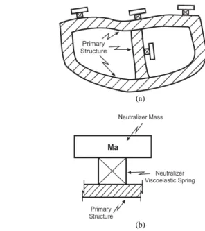
q generalized coordinate. The index j may be omitted when unnecessary, for ease understanding. Fig. 1 shows a structure of general shape with some absorbers attached to it.
The idea behind the attachment of a set of neutralizers on a primary structure is to reduce its responses to the action of input forces, or input displacements. How to design such a set of absorbers to achieve the best possible vibration abatement for a particular material, given in advance, is described in the sequel.
(a)
(b)
Figure 1. (a) Primary structure with absorbers attached to it. (b) A particular absorber.
Review of Generalized Quantities for an Absorber
For completeness, and ease reading of the paper, a brief review of the concept of generalized quantities for a simple vibration neutralizer, or absorber, is presented here (see Espíndola and Silva, 1992).
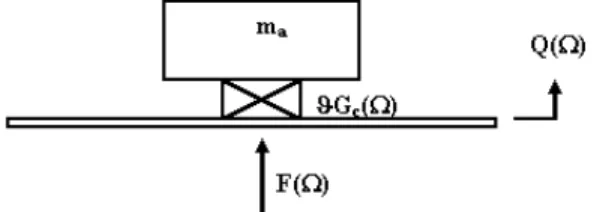
The simple absorber (the one degree of freedom absorber) has a single lump of mass (ma) connected to the primary structure through
a resilient device (a “spring”, see Fig. 2), assumed as having a viscoelastic nature, with complex stiffness ka(Ω) equal to (Espíndola,
1995):
( )
( )
( )
a c
k = Gϑ = Gϑ 1+ iη (14) The base plate in Fig. 2 is assumed massless in this analysis, with no loss of generality. In the above expression, Gc
( )
Ω is the complex shear modulus of the viscoelastic material, G (Ω) is the dynamic shear modulus, η(Ω) is the loss factor of such material, Ω is the circular frequency and ϑ is a geometric factor, depending on the shape and metallic inserts of the viscoelastic spring.Figure 2. Scheme of a simple (single degree of freedom) absorber.
In Fig. 2, Q(Ω) and F(Ω) stand for the Fourier Transforms of the basis displacement q(t) and the applied force f(t), respectively. This applied force is a result of the interaction between the absorber and the point of the primary structure where it is attached.
It is a simple matter to verify that the interaction force F(Ω) at the attachment (massless) plate “feels” the neutralizer as a dynamic stiffness given by:
( )
( )
( )
( )
2 a
a 2
a
m G 1+ iη
F( ) k ( ) = =
Q( ) m G 1+ iη
Ω ϑ
Ω
Ω
Ω Ω − ϑ (15)
The anti-resonant frequency of the simple absorber is defined as the one that, in the absence of damping (η( )Ω =0), makes the denominator of Eq. (15) equal to zero:
2
a= G( a) ma
Ω ϑ Ω (16)
In Eq. (16), Ωa stands for the anti-resonant frequency of the
absorber. In that equation, ϑ ΩG( a) is the stiffness of the viscoelastic spring at the anti-resonant frequency Ωa. Note also that Eq. (16) is a
transcendental equation for the anti-resonant frequency of the absorber.
Since it is possible to write G ( )c Ω =G(Ωa)r ( ) 1a Ω
[
+ η Ω( )]
, Eq.(15) can be rewritten as:2
2 2 2 2
a a a a a a
2
a a
3 2 a a a
k m
D ( )
i m
D ( )
r ( ) r ( ) r ( ) ( )
( )
r ( ) ( )
(17 )
+ = − Ω
Ω Ω
+ Ω
Ω
Ω Ω − Ω Ω Ω Ω Ω η Ω
Ω +
Ω Ω η Ω
where r ( )a Ω = ΩG( ) G(Ωa) and
( )
2( )
2 2( )
2( )
2a a a a
D Ω = Ω r Ω Ω- + η Ω Ω r Ω .
Now imagine a single degree of freedom system in which a mass m is connected to a fixed reference (“earth”) through a viscous dashpot of constant c. If a force f(t) is applied to the mass, this mass will respond with displacement x(t). The ratio between the input force and output motion, in the frequency domain, will be
( ) ( ) ( )
2k Ω = ΩF / X Ω = −Ω m i c+ Ω . If this equation is now compared with Eq. (17), one can see that the primary structure “sees” the absorber at the point of attachment as a mass m ( )e Ω connected to a viscous dashpot of constant c ( )eΩ , the other end of this dashpot being connected to the “earth”.
Figure 3 shows this interpretation. These two quantities are called here equivalent generalized mass and equivalent generalized viscous damping constant for the particular absorber. Dividing out
both numerator and denominator of Eq. (17) by 4 a
Ω, the equivalent quantities for the absorber can be written as:
3
a a
e a a 2 2
2
a a a
c ( ) m r ( ) ( ) r ( ) r ( ) ( )
= Ω η Ω ε
Ω Ω
ε − Ω + Ω η Ω
(18)
and
{
2 2}
a a a
e a 2 2
2
a a a
m m
r ( ) r ( ) 1 ( ) ( )
r ( ) r ( ) ( )
=
Ω Ω + η Ω − ε
Ω
ε − Ω + Ω η Ω
(19)
where ε = Ω Ωa a.
It is a simple task to lift the hypothesis of massless base plate for the absorber and consider its mass in Eq. (17).
Now, it has been proved that both schemes shown in Fig. 3 are dynamically equivalent (Espíndola and Silva, 1992) in the sense that the stiffness “felt” by the primary system is the same in both cases. The primary system “feels” the absorber as a mass m ( )e Ω , dependent on frequency, attached to it along a generalized coordinate q(t), and a viscous dashpot (even if the damping is of viscoelastic nature) of constant c ( )e Ω (also dependent on frequency) linked to earth (a fixed reference). The dynamics of the resultant system (primary + absorbers) can then be formulated in terms of the original physical generalized coordinates alone (of which Q(Ω), in Fig. 3, is a representative coordinate), although the new system has now additional degrees of freedom (one for each absorber). This is a fundamental property of the concept of equivalent generalized quantities for the absorbers.
Figure 3. Equivalent systems.
The Response of the Compound System
It can now be concluded from the previous discussion (and Fig. 3 helps this interpretation) that a linear structure modelled with many degree of freedom will have its damping and mass matrices modified (see below) by the attachment of the absorbers, but not their size. If the primary system has been modelled as an n degree of freedom structure, both damping and mass matrices will still be of order n×n after the attachment of the absorbers, in spite of the fact that p (p absorbers) new degrees of freedom have been added to it. As for the stiffness matrix, it remains unchanged after the attachment of the absorbers. Notice that Eqs. (18) and (19) contain all the parameters of the fractional viscoelastic model. So, if such p absorbers with equivalent generalized masses
e1 e2 ep
m ( ), m ( ),..., m ( )Ω Ω Ω and equivalent damping constants
e1 e2 ep
primary system along the generalized coordinates
1 2 p
k k k
q , q ,..., q , the equations of motion can be written, in the frequency domain, as:
2
i ( ) ( )
Ω + Ω +
− M C KQ Ω = ΩF (20)
where M and C are the modified mass and damping matrices, given by: ; e1 ep e1 ep = = + = + 0 c ( )
= + = + ( )
c ( ) 0 0
m ( )
( ) m ( )
0
Ω
Ω
Ω
Ω
Ω
Ω
A A M
M M M
C C C C
(21)
where C and M are the ordinary viscous damping and mass matrices of the primary system, respectively. Matrices MA(Ω) and CA(Ω) are
diagonal and complex. Notice that the entry
(
k , kj j)
is mej( )
Ω in( )Ω
A
M and cej
( )
Ω in CA( )Ω , j = 1, p. Notice also that a particulargeneralized quantity is given by (see Eq. (18) and Eq. (19)):
3 aj aj
ej aj aj 2 2 2
aj aj aj
c ( ) m r ( ) ( ) , j 1, p r ( ) r ( ) ( )
= Ω η Ω ε
Ω Ω =
ε − Ω + Ω η Ω
(22)
{
2 2}
aj aj aj
ej aj 2 2 2
aj aj aj
m m
r ( ) r ( ) 1 ( )
( ) , j 1, p
r ( ) r ( ) ( )
=
Ω Ω + η Ω − ε
Ω =
ε − Ω + Ω η Ω
(23)
where the index j stands for the jth neutralizer. Note also that
aj aj
ε = Ω Ω and r ( )ajΩ =G( ) G(Ω Ωaj), where Ωaj is the anti-resonant frequency of the jth absorber.
The anti resonant frequencies of the absorbers will be given by the equation below:
2 aj
j a j a j
; j = 1, p
G ( ) m
ϑ Ω
Ω = (24)
Now solve the following eigenvalue problem Kφφφφ = Ω2 Mφφφφ, involving the ordinary mass and stiffness matrices of the primary system, and define the modal matrix
1 2 m
r r r
= φ φ φ
Φ ,
containing only m eigenvectors
k
r
φ , k = 1, m. It is assumed that the corresponding band
1 m
r, r
Ω Ω
covers all the frequencies where the
vibrations are to be abated and that m << n. Note that Φ∈ ℜn m× .
Assume that all the eigenvectors are orthonormalized so that
=
T m
Φ MΦ I and ΦTKΦ=ϒϒϒϒm, where
(
1 2 m)
2 2 2
m =d ia g r r r
ϒϒϒϒ .
Now, in Eq.(20), apply the following transformation:
( )
Ω =( )
ΩQ ΦP (25)
If Eq. (25) is taken into Eq. (20), and this pre-multiplied by ΦT,
one gets, assuming proportional damping in the primary system:
{
2}
( )
( )
m
- MA( ) + i Γm+CA( ) + ϒϒϒϒ P =ΦTF (26) where
(
)
(
)
( )
( )
( )
( )
1 2 m
1 1 2 2 3 3
m m
2 2 2
r r r
r r r r r r
;
2ξ 2ξ 2ξ ;
;
diag diag
=
Ω = Ω
Ω + Ω
= = A A A A T m T
M I M
C Φ C
Φ Φ Φ Γ ϒϒϒϒ (27) Above, k
r, k 1, m
Ω = are undamped natural frequencies of the primary structure and
k
r , k=1, m
ξ are the corresponding modal damping ratios. Eq. (26) represents a small system of m << n equations and can be solved directly for any frequency with use of Eqs. (22) and (23). But this may not be the best way to follow, since matrices ( )
A
M and CA
( )
are not diagonal. Instead, a more robustapproach will be offered. Eq. (26) can be written in the following augmented way:
( )
( )
( )
( )
( )
( )
( )
( )
( )
m i i i Ω + Ω Ω
Ω +
Ω Ω
Ω
Ω
Ω
+ − Ω Ω Ω =
A m A
A
T A
P
C Γ M
P
M 0
0 P Φ F
0 M P 0
ϒϒϒϒ
(28)
or
( )
( )
( )
iΩΑY Ω +BY Ω =G Ω (29)
where
( )
( )
( )
; Ω + Ω
=
Ω
A m A
A
C Γ M
A M 0
( )
m ; = − Ω
A
0 B 0 M ϒϒϒϒ
( )
( )
( )
;( )
( )
i Ω Ω
Ω = Ω =
Ω Ω
T
P Φ F
Y G
P 0
.
The second set of equations in Eq. (28) is, in fact, an identity. Note that Ã, B∈ 2m×2m and Y(Ω), G~ (Ω)∈ 2m×1. Note also that a time
domain version of Eq. (29), say Ay
( )
t +By( ) ( )
t =g t , where( )
t = −1(
( )
Ω)
y F Y and g
( )
t =F −1(
G( )
Ω)
, cannot be written simply because both matrices A and Bare functions of frequency. This mixing of time and frequency domains would generate a set ofIt is not difficult to show that matrix B is positive definite. Consider the following eigenvalue problem, for a particular value of frequencyΩ:
θ = λ θ
B Α (30)
and define the following modal matrix Θ= θ θ
[
1 2 θ2m]
anddiagonal spectral matrix Λ2m=diag
(
λ1 λ2 λ2m)
. Assume thatthe eigenvectors are orthonormalized such that T =
2m
Θ AΘ I and
=
T
2m
Θ ΒΘ Λ and make the following transformation:
( )
Ω =( )
ΩY ΘZ (31)
This transformation is possible because the columns of Θ are linearly independent, which makes this matrix non-singular. In fact, the inverse of Θ is Θ−1=ΘTA.
Substituting for Y
( )
Ω into Eq. (29) and pre-multiplying by ΘT, one have:(
) ( )
T( )
iΩI2m+Λ2m Z Ω =Θ G Ω (32)
Solving Eq. (32) for Z
( )
Ω , substituting the result into Eq. (31)and remembering that Y
( )
Ω =P( )
Ω iΩ ΩP( )
T, one can get:( )
[
](
)
1[
]
T( )
11 12 i
−
Ω = Ω + T Ω
2m 2m 11 12
P Θ Θ I Λ Θ Θ Φ F (33)
Taking this result to expression 25, the following is obtained:
( )
Ω =(
iΩ +)
−1 T( )
Ω2m 2m
Q Ψ I Λ Ψ F (34)
where Ψ=Φ Θ
[
11 Θ12]
and[
Θ11 Θ12]
is the upper half of thematrix Θ. The matrix
( )
(
)
1 Ti −
Ω = Ω 2m+ 2m
Α Ψ I Λ Ψ (35)
is the so called receptance matrix and is a model of the compound system in the frequency domain. Note that A(Ω)∈ n×n. Having the receptance matrix for any frequency, the response at that frequency can be computed by:
( )
Ω =( ) ( )
Ω ΩQ Α F (36)
The sth column of the receptance matrix
( )
ΩA is given by the
expression (37):
( )
2m sjs j
j j 1= i
ψ
α Ω = ψ
Ω + λ
∑
(37)It is assumed that a convenient viscoelastic material is available, its four fractional parameters are known from experiment, and that all the absorbers are to be constructed with that same material. Since a modal model of the primary structure must also be known for the design process, it is assumed that the number and place of attachment of the absorbers have been decided beforehand. The obvious places of attachment for the absorbers are the points of maximum displacement in each mode within the band of interest. An absorber placed at a nodal line of a mode will be completely inefficient in reducing vibration at that particular mode.
The receptance matrix relates the vector of excitations to the vector of displacement responses, all in the frequency domain.
The relation between the vector of excitations and the vector of velocity responses is given by the so called mobility matrix
( )
Ω = i Α( )
M , and if acceleration responses are considered, the inertance matrix is called upon:
( )
2( )
( )
i
Ω = −Ω A Ω = Ω Ω
I M .
So, assuming p absorbers attached to the primary structure, the theory described above tells how to compute the response of the compound system. But the problem at hand is the reverse: having a primary system strongly responding to input excitations, how to design a set of dynamic absorbers so as to mitigate the vibrations to acceptable levels.
Specification of Absorbers Masses
For primary systems with only one degree of freedom, the recommended ratio between the absorber mass (ma) and primary
structure mass (ms) by Den Hartog (1956) is µ = ma /ms = 0.1 to
0.25. The use of the modal mass ratio concept has been proposed by Espíndola and Silva (1992) for a system of multiple degrees of freedom as:
i j
j
j
p 2 ai k s i 1 s
s m
, j 1, d m
= φ
µ = =
∑
(38)
where m is the mass of the iai th absorber and d is the number of modes taken inside the band of frequencies (d is, in general, smaller than m, the number of eigenvectors kept from problem Kφ = Ω2Mφ).
The symbol
j
s
m stands for the th j
s modal mass of the primary system, which, in case of orthonormalization of eigenvectors, is equal to one. The quantity
i j
k s
φ represents the element of Φlying in
the th i
k line and sthj column. The numbers k , ii =1, p are of the
coordinates qki, where the p absorbers are fixed to the primary
structure. So, given
j
s
µ , one for each of the modes of interest, a set of equations is established and m , i = 1, p are computed by SVD ai decomposition of the system matrix associated with Eq. (38). The matrix of the system shown in Eq. (38) is of order d p× . Note that the number of modes to be controlled (d) inside the band of eigenvectors in Φ∈ ℜn m× may be smaller, equal to or greater than
the number of absorbers (p) attached to the primary system. This means that the system of Eq. (38) may be underdetermined, over determined or determined.
The arguments leading to Eq. (38) are too lengthy and can be found in Espíndola and Silva, 1992.
Optimization for a Frequency Range
In what follows, it is assumed that a particular material is at hand, given by its four fractional parameters {α, b, G0, G∞}. In a
different approach, the material (i.e., the four parameters) is searched for in the process of designing an optimum system of viscoelastic absorbers (see Espíndola and Cruz, 2005).
anti-resonant frequencies Ωaj, j = 1, p in such a way that a norm of P(Ω) becomes a minimum. In such manner the response given by Eq. (34) is also minimized. Define x as a vector of anti-resonant frequencies:
T
ap a1 a 2
= Ω Ω Ω
x (39)
From Eq. (33), one has
( )
Ω = T( )
ΩP VΦ F (40)
where
(
)
1 Ti −
= Ω 2m+ 2m
V Ψ I Λ Ψ , for simplicity.
Since the Frobenius norm of a matrix is a consistent one, the following expression is valid:
|| P(Ω)||2 = || VΦΦΦΦT F(Ω) ||F ≤ || V ΦΦΦΦT ||F || F(Ω) ||F ≤
≤ || V ||F || ΦΦΦΦT ||F || F (Ω) ||2.
Since T F
Φ is a positive constant number and ||F(Ω)||2 is fixed
for every frequency, minimizing ||P(Ω)||2 means minimizing ||V||F,
for each and every frequency. So, take the following objective function:
( )
( )
max
min F
f max ,
Ω ≤Ω≤Ω
= Ω
x V x (41)
and minimize it. Note that V(Ω, x) is precisely the matrix
(
)
1 Ti −
= Ω2m+ 2m
V Ψ I Λ Ψ with Ω and x in evidence. Remember also
that x in Eq. (41) is the vector defined in Eq. (39).
As always, the better the information at hand, the better the results will be. One should expect then that the results obtained using this definition of objective function (where no information about the input vector is used) are more conservative than those obtained by using the previous one in Espíndola and Cruz (2005). This is a price to be paid for our ignorance. The advantage of this present objective function is that it ignores the input excitation, which may be crucial in certain applications.
After a minimization procedure of f(x), the p anti-resonant frequencies Ω Ωa1, a 2 Ωap for the p respective absorbers are known. Since
a j
m , j = 1, p were given as input parameters, the ϑj, j = 1, p
parameters of the viscoelastic element can be computed at each frequency
aj
Ω , j = 1, p, from Eq. (24). This is only a geometric factor. It is now left to the designer to give shape and size to the absorbers, so as to meet these anti-resonant frequencies and geometric factors.
For a uniform viscoelastic pad working in compression, it can be shown that
(
2)
3 1+βS A =
e
ϑ (42)
where A is the one side load carrying area, e is the thickness, and β is a factor equal to 2 for circular and square pads, and approximately 2 for moderately rectangular pads. S is the so called shape factor and is defined as the ratio of the one side load carrying area to the free surface area. For a symmetric arrangement of viscoelastic shear elements, like the one shown in Fig. 4, an approximate expression for the geometric factor is:
( )
n e i
, 0 2
e r / r
ϑ= ϕ < ϕ ≤ π, (43)
where e is the thickness of the viscoelastic elements, re and ri are the external and internal radius, respectively, ϕ is the sum of all angles, in radians, comprised by the viscoelastic sectors and n( )⋅ stands for the natural logarithm function.
Figure 4. Sketch of a simple viscoelastic vibration absorber working in shear. The internal cylinder is to be fixed on the primary structure. The external cylinder stands for the mass ma.
In the design practice, it may be convenient to make equal the resilient parts of all the absorbers. This calls for choosing the most significant (in a certain sense) of the form factors ϑj, j = 1, p (say
ϑ ), and then computing again the absorber’s masses: aj
aj 2
aj G ( )
m , j 1, p
( )
ϑ Ω
= =
Ω . (44)
A possible criterion is to specify ϑ as the rms value of all ϑj,
j = 1, p.
Making the resilient parts equal for all the absorbers may signify an important saving in money (for instance, in moulding and curing dies). This is clearly an approximation, often dictated by economy. The final result must then be checked. Simple as it is, this last approach may give excellent results as shown in Espíndola and Bavastri (1995, 1997a, 1997b and 2003).
Absorbers working in shear are in general very small in size (a few grams to few kilograms) and are normally designed to be applied to vibrating light surfaces (such as machine casings) to reduce vibration response and noise radiated from them.
Example: Reduction of Vibration in an Automobile Door
An automobile door, and in fact any car body panel, is an example of a vibrating structure where the exciting energy may come in through several points and yet none of them are quite distinct and clear to be considered in an analysis as an input point.
To properly design a system of vibration absorbers, a modal model of the primary system must be available. In the present case, this model was constructed both by finite element technique and by experimental identification. The finite element model was carried out with the purpose of finding the three best possible places for shaker excitation in the experimental identification work as well as the points for the application of absorbers. Also, a comparison with experimental natural frequencies was welcome. But no updating technique was used nor felt necessary in this work.
The finite element model consisted of 1106 shell elements divided in a quite fine mesh with 1374 nodes. The band of frequencies here considered ranged from 200 Hz to 1800 Hz. Twenty-five modes of vibration were found in this band of frequency.
The experimental identification technique was carried out in the same frequency band above quoted with a sampling frequency of 5000 Hz. To keep the white noise excitation within that band of frequencies, a digital filter FIR was designed with 60 dB rejection on both sides of the passing band. Eighty-two points of measurements, some of them coinciding with nodes of the finite element mesh, were selected together with three points of excitation, all of them shown in Fig. 5b. The excitation points are shown there as f , f , f1 2 3. The set up for experimental identification is shown in Fig. 5a. After acquiring all the FRFs, a global modal analysis was carried out.
The knowledge of the modal damping ratios of the primary structure is vital to a realistic evaluation of the efficacy of a damping treatment or of any other technique for reduction of structural resonant vibration response. That is why a modal experimental identification technique is so crucial. As is well known, no finite element technique can provide information on the inherent damping of the primary structure. The loss factors of the 25 modes within the frequency band were identified and they ranged from 0.00170 to 0.00610, which means a very low damped structure indeed. The identified natural frequencies were in very close agreement with those found by finite element technique.
Having identified the natural frequencies and modal damping within the band of interest, the ground was then prepared for the design of the four absorbers, according to the explanation given before. These had the form given in Fig. 4. They were fixed at points number 27, 45, 58 and 65, in Fig. 5b. They had all the same mass of 0.128 grams and resonant frequency fa=1239 Hz. Note that the mass of the absorbers is, in fact, a sort of average, as well as the frequency. It is done so for economic reasons in the process of absorbers production. The optimization process for the design of the absorber used a hybrid technique (genetic algorithm and David-Fletcher-Powell non-linear optimization approach; further details can be found in Bavastri et al., 1998).
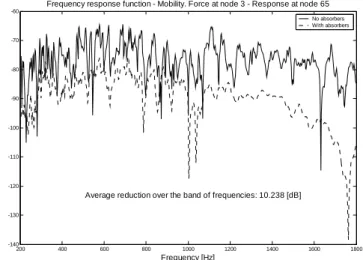
Figure 6 shows the average reduction, in dB, of the vibration response over a band of frequencies ranging from 200 Hz to 1800 Hz.
The four vibration absorbers were attached to the door at points corresponding to the largest amplitudes at that range of frequencies. The attachment of the four absorbers implied an increase in the mass of the door of 3.8%. The band of frequencies above was selected taking into account that the human ear is most sensitive at frequencies around 1 kHz.
(a)
(b)
Figure 5. (a) Set up for modal analysis of an automobile door. (b) View of an automobile door.
It can be seen in Fig. 6 an average reduction of 10 dB, which is a lot. Taking the average over all the averages, one for each frequency response, it was noted that a figure of about 10 dB reduction was typical of this particular treatment.
The standard practice in the automotive industry is to reduce vibration of automobile panels by sticking damping tapes (deadeners, in the jargon of automotive industry) on to them. A test
200 400 600 800 1000 1200 1400 1600 1800 -140
-130 -120 -110 -100 -90 -80 -70 -60
Frequency [Hz] A
bs olu te v alu e o f Mo bili t y [d B ] r e[1 m/s . N]
Frequency response function - Mobility. Force at node 3 - Response at node 65
No absorbers With absorbers
Average reduction over the band of frequencies: 10.238 [dB]
Figure 6. Vibration reduction shown by one of the frequency response functions.
200 400 600 800 1000 1200 1400 1600 1800
-120 -110 -100 -90 -80 -70 -60
Frequency [Hz] A
b s olu te v alu e o f Mo bili t y [d B] r e[1 m/s . N ]
Frequency response function - Mobility. Force at node 3 - Response at node 65
Door without damping tape Door with damping tape
Average reduction over the band of frequencies: 1.021 [dB]
Figure 7. Vibration reduction due to the original tape treatment on a car door.
In fact, a 10 dB reduction in such panels is quite a lot. Perhaps one would be content with a much smaller reduction, which would mean still much lighter dynamic vibration absorbers.
This discussion shows how powerful vibration absorbers are in mitigating structural vibration in structural panels. This also shows the great potential of viscoelastic vibration absorbers in reducing sound radiation from structural panels.
Conclusions
A brief, but adequate, account of the theory of fractional derivative models for viscoelastic materials has been provided in this paper, both for completeness and pedagogical reasons.
The general theory for the design of systems of viscoelastic vibration absorbers, developed by the authors over many years, has been reviewed, also with the purpose of clarity and ease reading. It assumes that a particular viscoelastic material is available beforehand and known by its four fractional parameters, identified experimentally. It also assumes that a modal model, albeit incomplete, of the primary system is identified.
The experimental identification of a modal model of the primary system is of absolute necessity, for it is rather important that the
modal damping ratios are known with great accuracy. As it is well known, finite element techniques are unable to provide such modal damping ratios. Failure to identify the modal damping ratios accurately make it difficult, if not impossible, to draw a realistic assessment of the set of viscoelastic absorbers in vibration and radiated noise abatement.
A novel objective function, based on a Frobenius norm, has been introduced here. This norm allows for the design of a system of viscoelastic vibration absorbers without knowledge of the set of exciting forces and their application points.
The theory, together with this new objective function, has been applied to an automobile door, with remarkable results as compared to those obtained with damping tape.
References
Bagley, R. L. and Torvik, P. J., 1979, “A generalized derivative model for an elastomer damper”. The Shock and Vibration Bulletin, Vol. 49, No. 2, pp. 135-143.
Bagley, R. L. and Torvik, P. J., 1983, “Fractional calculus – a different approach to the analysis of viscoelastically damped structures”. IAAA Journal, Vol. 21, No. 5, pp. 741-748.
Bagley, R. L.and Torvik, P. J., 1986, “On the fractional calculus model of viscoelastic behaviour”. Journal of Reology. Vol. 30, pp. 133-155.
Bavastri, C. A., Espíndola, J. J. and Teixeira, P. H., 1998, “A hybrid algorithm to compute the optimal parameters of a system of viscoelastic vibration neutralisers in a frequency band”. Proceedings of MOVIC’98, Zurich, Switzerland, pp. 577-582.
Broch, J. E., 1946, “A note on the damped vibration absorber”. Journal of Applied Mechanics, Trans. ASME. Vol. 68, pp. A284-.
Candir, B. and Ozguven H. N., 1986, “Dynamic vibration absorbers for reducing resonance amplitudes of hysterically damped beam”. Proc. of the 4th International Modal Analysis Conference, Los Angeles, USA, pp. 1628-1635.
Crandall, S. H., 1970, “The role of damping in vibration theory”. Journal of Sound and Vibration, Vol. 11, No. 1, pp. 3-18.
Crede, E. C. (1965). “Shock and Vibration Concepts in Engineering Design”. Prentice-Hall, Inc., Englewood Cliffs, NJ, pp. 121-.
Den Hartog, J. P., 1956, “Mechanical Vibrations”. New York: McGraw-Hill. Esmailzadeh, E. and Jalili, N., 1998, “Optimum design of vibration absorbers for structurally damped Timoshenko beams”. ASME Journal of Vibration and Acoustics, Vol. 120, pp. 833-841.
Espíndola, J. J., 1995, “Notes on viscoelastic damping” (in Portuguese). UFSC, Florianópolis, SC, Brazil.
Espíndola, J. J. and Bavastri, C. A., 1995, “Reduction of vibrations in complex structures with viscoelastic neutralizer: a generalized approach”. Proceedings ASME Design Engineering Technical Conferences, Boston, USA, Vol. 3, Part C, 761-766.
Espíndola, J. J. and Bavastri, C. A., 1997a, “Reduction of vibrations in complex structures with viscoelastic neutralizers: a generalized approach and a physical realization”. Proceedings ASME Design Engineering Technical Conferences, Sacramento, California, Paper DETC97/VIB-4187, in CD ROM.
Espíndola, J. J. and Bavastri, C. A., 1997b, “Viscoelastic neutralisers in vibration abatement: a non-linear optimisation approach”. Journal of the Brazilian Society of Mechanical Sciences and Engineering. Vol. 19, No. 2, pp. 154-163.
Espíndola, J. J. and Bavastri, C. A., 2003, “Modal reduction of vibrations by dynamic neutralizers in a frequency band”. In: VI Symposium on Dynamic Problems of Mechanics. Vol. 1, pp. 214-217.
Espíndola, J. J., Bavastri, C. A. and Lopes, E. M., 2008, “Design of optimum systems of viscoelastic vibration absorbers for a given material based on the fractional calculus model”. Journal of Vibration and Control, Vol. 14, No. 9-10, pp. 1607-1630.
Espíndola, J. J. and Silva, H. P., 1992, “Modal reduction of vibrations by dynamic neutralizers”, Proc. of the 10th International Modal Analysis Conference, San Diego, CA, USA: pp. 1367-1373.
Espíndola, J. J., Silva Neto, J. M. and Lopes, E. M., 2004, “A new approach to viscoelastic material properties identification based on the fractional derivative model”. Proceedings of 1st FDA IFAC Workshop on
Espíndola, J. J. and Cruz, G. A. M., 2005, “On the design of optimum systems of viscoelastic vibration neutralizers”. In: Modeling and control of autonomous decision support based systems. Hofer E. and Reithmeier (eds), pp. 49-64.
Floody, S. E., Arenas, J. P., Espíndola, J. J., 2007, “Modelling metal-elastomer composite structures using a finite-element-method approach”. Journal of Mechanical Engineering, Vol. 53, No. 2, pp. 66-77.
Freitas, F. L. and Espíndola, J. J., 1993, “Vibration control of cantilever beams with beamlike dynamic vibration absorbers”. Proceedings of the 5th DINAME International Symposium on Dynamic Problems of Mechanics, Santa Catarina, Brazil, pp. 117-121.
Gaul, L., Klein, P. and Kemple, S., 1991, “Damping description involving fractional operators”. Mechanical Systems and Signal Processing, Vol. 5, pp. 81 – 88.
Jacquot, R. G., 1978, “Optimal dynamic vibration absorbers for Timoshenko beams”. M.Sc. Thesis in Mechanical Engineering, Sharif University of Technology, Tehran, Iran.
Korenev, B. G. and Reznikov, L. M., 1993, “Dynamic Vibration Absorbers”. New York: John Wiley & Sons.
Liebst, B. S. and Torvik, P. J., 1996, “Asymptotic approximations for systems incorporating fractional derivative damping”. Journal of Dynamic Systems, Measurement, and Control, Vol. 118, pp. 572-579.
Manikahally, D. N. and Crocker, M. J., 1991, “Vibration absorbers for hysterically damped mass-loaded beams”. ASME Journal of Vibration and Acoustics, Vol. 113, pp. 116-122.
Ormondroyd, J. and Den Hartog, J. P., 1928, “The theory of dynamic vibration absorber”. Journal of Applied Mechanics. Trans. ASME, Vol. 49, pp. A9-A22.
Pritz, T., 1996, “Analysis of four- parameter fractional derivative model of real solid materials”. Journal of Sound and Vibration, Vol. 195, No. 1, pp. 103-115
Rossikhin, Y. A. and Shitikova, V., 1998, “Application of fractional calculus for analysis of nonlinear damped vibrations of suspension bridges”. Journal of Engineering Mechanics, Vol. 124, No. 9, pp. 1029-1036.
Rutmann, R. S., 1995, “On physical interpretations of fractional integration and differentiation”. Theoretical and Mathematical Physics, Vol. 105, No. 3, pp. 1509-1519.
Snowdon, J. C., 1975, “Vibration of simply supported rectangular and square plats to which lumped masses and dynamic vibration absorbers are attached”. Journal of Acoustical Society of America, Vol. 57, No. 6, pp. 646-654.