J. Braz. Soc. Mech. Sci. & Eng. vol.31 número2

Marcelo Becker

!" #"" $ $ % &

Richard Hall

Sascha Kolski

' '

Kristijan Maček

( ' ' &

Roland Siegwart

) * + , - . / -0.

1 2 ,3, 0 4"56$ .7 $ ) & +

Björn Jensen

( ( '

- 8

9 : ;

0 " 2 $ ) & +

2D Laser based Probabilistic Motion

Tracking in Urban like Environments

Introduction

1_{As a result of the astonishing advances made over the last} decades on several scientific fields, today mobile robots have many real applications. They range from Automatic Guided Vehicles (AGVs) and Autonomous Mobile Robots (AMRs) on factory floors, personal assistants for disabled and elderly people to exploration of hazardous environments such as surface of planets and bottom of oceans. Wherever the robot may be and whatever its purposes are an interface to exchange information is always needed. For many applications, e.g. when the interaction between humans and robots are not close, this interface may be a simple remote control. On the other hand, when robots and humans interact directly or they need to be more autonomous and take decisions based on their perception of their environment, the interface might be much more complex. Autonomous behavior is frequently represented as a perception-reasoning-action loop. It means that given the specification of a goal, the robot uses perception to identify relevant elements, then it analyses them, plans tasks to attain the goal, and finally executes these tasks. More autonomous systems may even define the goal to be reached based on some criteria.

Recently, several events around the world and research funding agencies have been impelling robotics researchers to focus their works on developing, transferring, and adapting techniques and approaches initially developed for indoor and outdoor mobile robots to car-like autonomous mobile robots. Events such as the DARPA

Paper accepted January, 2009. Technical Editor: Glauco A. de P. Caurin

1st and 2nd Great Challenge (2005, 2007), ELROB (2005), and C-ELROB (2007) are paving the way for the use of promising technologies in military and civil vehicles (Thrun et al., 2006; Dahlkamp et al., 2006; Lamon et al., 2006; and Stavens et al., 2007). On the other hand, in a near future, an assistance system that helps the driver and acts mostly in peril situations will be implemented more easily when compared to a fully autonomous system and will probably be more attractive for the majority of the drivers (one should take into account that western people tend to be standoffish regarding robots, in severe contrast to the Japanese, who welcome ubiquitous machines).

Systems like the Intelligent Parking Assist (IPS) technology onboard the Toyota Prius are becoming very popular among car buyers. Due to this, many researchers are working on car-like robot autonomous parking problem. This is a perfect example of an assistive system that uses sensors, e.g. ultrasound sensors and cameras, to help the driver during maneuvers. This amounts to saying that a system which is able to provide a full parking maneuver procedure, without any human intervention, is desired and will shortly become a serial item. Another example is the Secure Propulsion using Advanced Redundant Control project – SPARC - developed at the Swiss Federal Institutes of Technology (EPFL and ETHZ) in cooperation with a European Consortium of Automotive Companies (Holzmann et al., 2005-a and 2005-b, and Becker et al., 2007-b). Recent developments on sensors, actuators, algorithms, etc. applied on intelligent vehicles can be found in SAE series PT-132 (2006) and PT-133 (2007).

substituted by hundred of vehicles virtually interconnected and moving autonomously in a cooperative way. Onboard computers are likely to work together and control completely the vehicles under any weather and road conditions. Nevertheless, in order to achieve this dream scenario, the entire road network and vehicle fleet need to be adjusted accordingly.

Taking into account that there are hundreds of millions of vehicles and road kilometers in the world, these changes possibly represent a cost of billions of dollars. In a near future, a less expensive solution is an intelligent road network based on road and onboard vehicle sensors and computers. In this case, adapted freeways monitor vehicles, road, and weather conditions act as an assistive system alerting the drivers for peril situations. Today this scenario is becoming a reality in Europe, Asia, and North America. Another option is the use of intelligent assistive systems (e.g.: anti-collision systems) onboard vehicles. In case of an imminent collision, the system would alert the driver or assume the vehicle control.

There are several problems to be solved in both cases (fully autonomous and assistive technologies), but recent developments of onboard hardware and sensors are resulting in considerable research progress. However, the best ratio between desired autonomous behavior and costs when selecting the onboard hardware and software necessary for acquiring, extracting, and interpreting the environment features is to be drawn. In the context of autonomous and assistive systems, the importance of cognitive abilities is noticeable. Similarly to persons that need their senses in order to interpret and interact with the environment, an autonomous robot needs sensors that would provide information about his vicinity and state. In practice, the interpretation of the scene (i.e.: environment feature extraction, robot auto-localization, obstacle position detection, obstacle classification, obstacle path prediction, etc.) is essential to provide the robot controllers with information to plan a safe path. Although sensor technology has experienced significant improvements recently, high dynamic changing and unconstrained environments still represent an enormous challenge for the robotics research community. This is the case of urban-like environments where traffic (car, buses, bicycles, etc.) and pedestrian paths are unknown and sometimes difficult to predict. In spite of this, the obstacle motion tracking is an indispensable procedure for improving the robot environment perception. Unfortunately, it is a difficult task when some obstacles close to the robot’s sensors may cause blind zones behind them. In this situation, the robot may lose vital information about hidden obstacles that could avoid future collisions.

Some examples of researches developed in the field of autonomous parking are those carried out by Chao et al. (2005), Khoshnejad M. and Demirli (2005), Yamamoto et al. (2005), and Chiu et al. (2005). In this topic, fuzzy logic and artificial neural networks are some of the approaches used by the authors to face the problem. In addition to these researches, the works developed by Wang and Thorpe (2002), Duan et al. (2004), Lee and Chen (2004), Lu and Chuang (2005), Martínez-Marín (2005), Romero-Meléndez et al. (2005), Thompson and Kagami (2005), Kolski et al. (2006), and Maček et al. (2006) addressed a more complex problem: the path-planning task in urban environments for car-like mobile robots. The hidden and visible obstacles tracking problem was addressed in Becker et al. (2007-a). Virtual drivers, drive-assistant systems, and lane detection using artificial vision systems were focused in Maček et al. (2004), Bellino et al. (2005), Holzmann et al. (2005-a and 2005-b), and Lamon et al. (2006).

The present work focuses the 2D laser-based obstacle motion-tracking problem in dynamic unconstrained environments (urban-like) by applying a Kalman Filter in order to predict the obstacle motions when they are hidden. This would allow the car-like mobile

robot controller to take into account hidden and non-hidden obstacles when maneuvering the robot. A probabilistic occupancy-grid representation of the environment was also implemented. It provides a given time horizon prediction view of the robot surrounds based on motion-models of the obstacle classes and obstacle-estimated velocities. Initially, the test platform (Smart Car) is presented. Next, a brief review of the state of art on motion tracking is addressed and the multi-obstacle motion-tracking algorithm (including the Kalman Filter) is shortly described. Then, the results obtained while using real data are shown. Finally, the conclusion and outlook are presented.

Nomenclature

ac = centripetal acceleration, m/s2 F = state transition matrix, - H = measurement transition matrix, - ICM = instantaneous center of motion, - L = distance between rear and front axles, m MD = Mahalanobis distance, m

n = data quantity, -

P = state covariance matrix, - Q = process noise covariance matrix, - r = turning radius, m

R = measurement noise covariance matrix, - S = innovation covariance matrix, - t = time, s

V = velocity, m/s

v _{= state vector, m and m/s}

w = measurement white noise, m W = filter gain, -

x = state vector, m and m/s

x = measured point x coordinate on a segment, m y = measured point y coordinate on a segment, m

xˆ = state prediction vector, m and m/s z = state vector, m and m/s

zˆ = state prediction vector, m and m/s

Greek Symbols

∆ = parameter variation, -

θ = steering angle, rad

µ = expected mean value, m

ν = innovation, m and m/s

σ = standard deviation, m

σσσσ = variance, -

υυυυ = process white noise, m

φ = angular orientation, rad

ϖ = angular velocity, rad/s

Subscripts

i relative to parameter indices max relative to maximum value min relative to minimum value norm relative to norm

X relative to stochastic variable Y relative to stochastic variable

Superscripts

Test Platform – Smart Car and Laser Range Finder

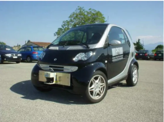
The Smart Car used as test platform is based on an ordinary smart fortwo coupé passenger car (Fig. 1). Obviously some changes and improvements were included in order to allow the vehicle autonomous behavior, e.g.: a steer-by-wire system (Fig. 2). Undoubtedly, the heart of the vehicle is the onboard computer. It is interfaced with several sensors and actuators that control the vehicle through the controller-area network (CAN). For instance, braking, acceleration, and steering controls are made by controlling dedicated motors. A system of cable and pulleys controlled by a motor is used to activate the brake pedal. An electronic system was designed to set the throttle command directly (the voltage, originally provided by the potentiometer in the throttle pedal, is generated by the computer and sent to the CAN).

Figure 1. Modified Smart Car used at ASL. Observe the LMS 291 SICK laser sensor assembled on its front bumper.

Torque sensor

Velocity (CAN) Torque (voltage)

Madd

Computer

Computer

CAN to analog

CAN to analog

Steering electronic board

Steering

Steering

electronic board

electronic board

Vehicle CAN

C

o

m

p

u

te

r

C

A

N

V

e

h

ic

le

C

A

N

Switch

Position controller (PID) Minimize : e = θθθθdesired–θθθθ

DA Unit

DA Unit

Torque sensor

Velocity (CAN) Torque (voltage)

Madd

Computer

Computer

CAN to analog

CAN to analog

Steering electronic board

Steering

Steering

electronic board

electronic board

Vehicle CAN

C

o

m

p

u

te

r

C

A

N

V

e

h

ic

le

C

A

N

Switch

Position controller (PID) Minimize : e = θθθθdesired–θθθθ

DA Unit

DA Unit

Figure 2. The steer-by-wire system implemented in the Smart Car.

A set composed by a steering encoder and a motor allows the computer to steer the vehicle front wheels. Summarizing, the vehicle CAN can access the following internal car state data:

1. Vehicle flags: engine on, door closed, brake pedal pressed, etc.;

2. Engine: engine rpm, instantaneous torque, gear shift, temperature, etc.;

3. Odometry: global vehicle speed, individual wheel speeds, ABS activated;

4. Throttle pedal value and steering wheel angle.

A switch enables to select the manual or autonomous vehicle modes. The Smart Car is also equipped with Global Positioning System (GPS) and 6 degree of freedom (DoF) Inertia Measurement Unit (IMU), allowing measuring the vehicle relative movement. The IMU measures lateral acceleration in all three dimensions, angular

rates up to 100º/s with a resolution of 0.025º, and lateral acceleration up to 2g with a resolution of 0.01 m/s2. Exteroceptive sensors, such as a monocular camera and a laser range finder (SICK AG Laser Measurement Sensor - LMS 291) both looking forward, have also been installed. The laser sensor was assembled on the front bumper of the Smart Car and it has a 180º field of view with an angular resolution from 1º to 0.25º. Its maximum range is 80 m and it has a statistical error of 10 mm.

In this work we used the data from the laser scanner as the main source of information. This choice was based on the fact that laser sensor prices are gradually decreasing every year, what may make it possible their commercial use in passenger vehicles in a near future.

Sensor Model

Laser scanners are active sensors that emit a laser beam and rely on the time-of-flight principle for measuring distance. A rotating mirror or prism is used in order to cover an angular range. The neighboring points are taken at successive rotations of the revolving unit. Thus, they are taken with a time difference proportional to the rotational frequency (fsensor) of the revolving unit (in our case,

fsensor = 75Hz). The sensor data flow can be understood as follows:

the laser sensor acquire data over a period of time ∆t, which is then

sent to the computer via RS422 where a real-time thread reads data at 17Hz. In a first step, the data set is transformed into a coordinate system centered on the vehicle and it is assigned with a time-stamp and the vehicle position at this time. Depending on the desired angular resolution, the acquisition time varies. For 0.5º resolution two rotations are necessary, so the acquisition time amounts to ∆t = 2/fsensor. During the first rotation the data points for the angular

position 1, 3,... are taken and the second rotation provides the even set of 2, 4,... When running in 0.25º mode even four rotations are necessary and the acquisition time amounts ∆t = 4/ fsensor.

In our case, the main objective of modeling the laser scanner is to take into account known sources of uncertainty while tracking the obstacles. The main assumption used is that different sources of error are pair wise independent and can be modeled as Gaussian distributions. Thus, the resulting uncertainty may be represented as its covariance (Jensen, 2004). There are several origins for laser measurements, but the main ones are: the timer counting the time-of-flight, the stability of the rotational frequency of the revolving unity and the frequency with which beams are sent out. Unfortunately, the sensor documentation (SICK AG, 2006) has no data for ranges greater than 20 m and for the angular uncertainty. For the experiments carried out in this research (0.5º angular resolution and 30 m range) we assumed the sensor data specified in the documentation for a 20 m range (the uncertainty on the distance measured to σρ2 = 0.012 m2). Concerning the angular uncertainty, in fact we observed that the angular values provided by the sensor are constant and taken from a table. Due to this, it is difficult to evaluate the angular uncertainty experimentally. So, we used the opening angle of the laser beam (0.5º) and assume the angular uncertainty to be half the beam width (σφ2 = 0.252º2). As previously cited, distance and angular uncertainties are assumed to be independent and Gaussian distributed, thus the sensor uncertainty is represented by:

) , ( diag

sensor 2 2

2

φ ρ σ σ =

σσσσ . (1)

Motion Tracking

and data uncertainty. In order to deal with these problems the use of Kalman Filters (KF) was proposed in the early 1960s by Kalman (1960), and Kalman and Bucy (1961). Early studies focused on single and multi-target tracking, and data origin uncertainty applied on environment surveillance also proposed the use of KF (Sittler, 1964; Sea, 1971; and Singer and Stein, 1971). When dealing with the incorporation of uncertainty on the data origin in tracking, one should keep in mind that the robot is dealing with multiple-hypothesis tracking. This means that it has a combinatorial explosion of hypothesis that usually cannot be handled in real-time (Jensen, 2004). There is a large quantity of publications in the literature related to motion tracking using a variety of sensors (vision, laser, etc.). As our test vehicle has an onboard 2D laser sensor used for extracting the environment data, we decided to focus our literature review on the development of systems that use mobile robots with onboard 2D laser sensors. Nevertheless, when it comes to car-like tracking applications in dynamic urban scenarios that use only 2D laser sensor data, literature proved to be scarce up to now. Pradalier et al. (2004) developed an interesting approach using as test vehicle a bi-steerable car called CyCab. However, they did not focus their research on multi-obstacle motion tracking, but on the integration of some essential autonomy abilities into a single application (simultaneous localization and environment modeling, motion planning and motion execution amidst moderately dynamic obstacles).

Considering indoor applications, there are several works that focused the motion-tracking problem based on 2D laser sensor data. Shulz et al. (2001) addressed the application of multi-obstacle motion tracking algorithms onboard mobile robots for tracking moving persons. They applied a sample-based representation of the joint probability density function (SJPDF) of all moving obstacles to avoid the combinatorial explosion of multi-hypothesis tracking. If on the one hand they could combine SJPDF with a local occupancy grid and show the tracking of several persons through temporal occlusions in well structured environments, on the other hand, the use of SJPDF requires the knowledge of the tracked obstacle quantity. It means that they needed to use a Bayesian filter and the time sequence of moving features quantity to estimate the tracked obstacle quantity. At the end, their motion tracking algorithm had to deal with local minima, non-linear relations due to the increased occlusion quantity, local occupancy grids, and the use of probabilistic filters to filter static objects that could become difficult to handle in real-time for non-structured environments. Kluge et al. (2001) presented a strategy for analyzing the robot-human interaction scenario. It was based on a set of prototypical situations in crowded public environments and consists of scene analysis, tracking, action recognition, and intention reasoning procedures. Illmann et al. (2002) extended this analysis by applying local person density and tree-based vector quantization. Bennewitz et al. (2002-a and 2002-b) developed a system to segment tracks of a person in a common household environment. In this work, the trackers were obtained from static laser sensors and the segmentation process was based on Expectation Maximization approach. Their purpose was the detection of the intention of a person based on his or her path. Jensen (2004) addressed the multi-object tracking problem using single Kalman Filters for each individual problem. In order to deal with data association he used validation gates and to solve the measurement-track assignment he utilized linear programming techniques. Our approach is based on (Jensen, 2004) and extends it for urban-like environments focusing on tracking pedestrians and vehicles (e.g.: cars, trucks, and buses).

Outputs

Tracking

Detection

Scan Raw Data

Scan Raw Data

Segmentation

Segmentation

Obstacle and Features Extraction

Obstacle and Features

Extraction _DetectionMotion Motion Detection

Local Occupancy

Grid Map

Local Occupancy

Grid Map

Data Association

Data Association

Initiate a New Tracker

Initiate a

New Tracker Update _Tracker Update Tracker

Predicted Occupancy

Grid Map

Predicted Occupancy

Grid Map

Trackers

Trackers

Outputs

Tracking

Detection

Scan Raw Data

Scan Raw Data

Segmentation

Segmentation

Obstacle and Features Extraction

Obstacle and Features

Extraction _DetectionMotion Motion Detection

Local Occupancy

Grid Map

Local Occupancy

Grid Map

Data Association

Data Association

Initiate a New Tracker

Initiate a

New Tracker Update _Tracker Update Tracker

Predicted Occupancy

Grid Map

Predicted Occupancy

Grid Map

Trackers

Trackers

Figure 3. Flowchart representing the General Structure of the Motion Tracking Algorithm.

Figure 3 summarizes the approach developed for urban-like environments. The 2D laser raw data acquired by the SICK laser sensor are used as input data for the obstacle detection algorithm. Initially, the data are segmented in order to extract the environment features and to detect motion. Features that are not moving are considered static and stored in a local map that is also used for detecting motion. After detecting mobile obstacles, a process of data association is applied to start new trackers or update existing trackers. Trackers that are hidden for more than a threshold value (e.g.: one second) are deleted. Put simply, the whole procedure outputs are:

1. Non-hidden obstacle quantity, obstacle positions and estimated velocities (Trackers in Fig. 3);

2. Hidden obstacle quantity, obstacle predicted positions and velocities (Trackers in Fig. 3);

3. Obstacle classification, e.g. pedestrian, car, truck, etc. (Trackers in Fig. 3);

4. Local Occupancy Grid Map;

5. Predicted Occupancy Grid Map for a given time horizon (e.g.: 1 second).

Both procedures, obstacle detection and tracking, are shortly explained as follows.

Obstacle Detection

There are several approaches for detecting objects using a 2D laser scanner in the literature, most of them centered in indoor mobile robotics applications. For a fixed sensor this task is straightforward since it is possible to compare two consecutive scans and immediately determine which points remains in the same spot and which do not. For a mobile sensor like the one onboard a mobile robot or a vehicle such as a car, the task is somewhat more difficult due to the translation and rotation caused by its displacement. Take for example a static obstacle that is seen by only one point in the first scan. In the next scan the sensor has moved a little and the changed viewing angle results in the point being seen at another spot on the same obstacle. This phenomenon can give a false impression that the static obstacle is actually moving. In order to avoid this, it is necessary to take into account, as precisely as possible, the vehicle position. This work focuses on detecting moving obstacles like vehicles and pedestrians. To perform this task, we utilized the Motion Filter approach (Lindstrom and Eklundh, 2001; and Wang and Thorpe, 2002).

Lamon et al. (2006-a and 2006-b) and Kolski et al. (2007). Basically, in order to accurately localize the vehicle, the GPS, the IMU, and the wheel encoder data were combined using a Kalman Filter to estimate its 6 degrees of freedom, i.e. its position and attitude (Sukkarieh et al., 1999; and Dissanayake et al., 2001). This filter is called Information Filter (IF) and during the experiments it produced excellent results when the vehicle was traveling at low speeds in open areas (far from large structures, tunnels, etc.). The standard deviation of the filtered position was less then 0.025 m for all three position coordinates. Based on this result we decided to neglect the vehicle position uncertainty, while modeling the Kalman Filter used to estimate the obstacle motions when they are hidden (see Kalman Filter item). Following this premise, we could use directly the vehicle position estimated by the IF to produce local maps and detect motion, even when the vehicle was moving.

Segmentation

Grouping measurements that belong to the same object are mandatory, when processing data from a laser scanner. The scans will consist of length measurements at equidistant angles and therefore it is very likely that two points that are close to each other also belong to the same object. Likewise, two consecutive measurements that are far away are likely to imply that a change in the observed object has occurred. Since it is necessary to define a distance threshold, there is always the risk of making errors in the segmentation process, either by creating one single segment out of two or more close objects, or by dividing an object into more than one segment. The segmentation makes it possible to do further processing on the different segments or point clusters. This normally consists of classification by size, dynamic status, or geometrical features (MacLachlan, 2004).

Motion Based Approach

Basically, the idea is to compare two scans apart by some time interval, ∆t, trying to match them in order to determine which points

are static and which are dynamic. By using this approach one can suppress spurious readings from the static environment, giving a better input to the tracker. The scan matching is made by storing the previous scan and comparing it to the new one. For each point in the new scan, distances to points in the old scan are calculated and compared to a threshold value (in our case, ± 10 cm). If a match is found, the point is likely to be static. One exception is when points are matched to a different area on a moving obstacle, for instance along the side of a passing vehicle. This problem was later solved by checking the dynamic classification in the first scan. If a point was labeled dynamic at that time, it is likely to be dynamic in the next scan. However, if no match is found, one cannot say for sure that the point is moving without further processing. The point could have been occluded in the first scan or out of range due to vehicle motion between scans. Therefore, we make use of the free area that is the space between the robot and the obstacles or scan range. If a point seen in the second scan is not found but within this area in the first scan, thereby observable, it is labeled as moving. A segment containing a certain amount of points labeled as moving can be sent to the tracker, after its center point is calculated.

During the simulation phase, we observed that the simple use of scan matching was not sufficient to deal with spurious readings. One reason for this behavior was the translation and rotation movements of the sensor. Aiming to increase the detection of static points, a local map was created. At first, the map was implemented as a position vector, storing in each scan the coordinates of all points labeled as static ones. New scans were then checked against the map and when a match was found, the weight for that map point was

increased. In order to keep down the size of the map, each point kept track of its own age. When a terminal age was reached, e.g. after 10 seconds, the point would be deleted from the map. The static map helped to improve the motion detection, but some disadvantages were noticed. The representation of the map using points was one of them. Measurements are never exact, and therefore, it is difficult to determine how many map points are needed to represent an obstacle. If we add all new static points, we get a very large map which slows down the matching process. But if we only add points that were not matched to the map before, we will certainly miss useful information. A method that turned out to be a better approach to the local mapping was the Time Stamp Method (Fiorini and Shiller, 1998). Basically this method is an Occupancy Grid Representation (Elfes, 1989) that does not consider the uncertain cells. Due to this, only free and occupied cells are considered and the computational time necessary for each environment scan is reduced.

Thanks to the use of the Fiorini and Shiller’s occupancy representation, we could improve and simplify the scan matching process. Latter, the occupancy grid was used not only to represent the static environment, but also to represent present and future predictions of the tracker output. This was carried out by adding a probabilistic grid to the occupancy representation (see Predicted Occupancy Grid Map item). Due to this, it was necessary to classify and model the obstacles that were being tracked.

Obstacle Classification

By classification, we refer to the process of determining if a moving segment belongs to vehicles or pedestrians. While working with the MatLab Simulator (Becker et al., 2007-a), pedestrians were rarely detected by more than two or three scan data. Since the sensor is placed about 50 cm from the ground, it usually detects one point on each leg. If the pedestrian stands close to the sensor it is easier to distinguish a contour, but this was rarely the case. An obvious difference between vehicles and pedestrians is their size, so we decided to base the classification on it. We used the standard deviation of each segment to represent its size:

∑ =

= n

i i

X x

n ₁

1

µ _∑ =

= n

i i

Y y

n ₁

1

µ , (2)

∑

= −

= n

i X i

X ( x )

n 1

2 2 1 _µ

σ _∑

= −

= n

i Y i

Y ( y )

n 1

2 2 1 _µ

σ , (3)

where X and Y are stochastic variables, x and y are measured points

on a segment, n is the data quantity, and µ and σ are expected values and standard deviations respectively.

Checking the norm of standard deviations against a predefined threshold yields the classification into vehicle or pedestrian:

2 2

Y X

norm

σ

σ

σ

Obstacle Tracking

dynamic state of an obstacle, i.e. its position and velocity, and with this information predictions can be made on the obstacles future positions (Bar-Shalom and Fortmann, 1998; and Blanc et al., 2005). In an urban environment, laser measurements are subject to noise, which we have to suppress by filtering. It is also usual to expect obstacles being hidden by other obstacles. However, it is possible to continue to track these obstacles until they are seen again and thereby minimize the risk of a collision. Each obstacle in this setup is characterized by its center of gravity, or at least the center of gravity for the part that is being seen. Since the scanner provides a 2D output, this point is described by (x, y) coordinates. The x and y

velocities were also introduced in the state of the dynamic object for tracking the motion of each obstacle and predicting its continued path. The state vector then becomes:

x

v_state =(x x y y)T = . (5)

However, from now on we will simply denote it as x. The measurements, containing only the x and y values, are labeled z.

Kalman Filter

The Kalman Filter (KF) is a wide spread technique for estimating the state of a dynamic system observed through noisy measurements. The filter is a recursive state estimator, which means that in every step it uses the output of the previous step to make a new prediction. It consists basically of two steps, the prediction step when estimation is made based on the old state, and an update step when that estimation is updated with a new measurement. The state and measurement predictions are denoted by xˆ and zˆ. In order to predict a dynamic system response, a dynamic model is used. In this study the linear constant-velocity model (Jensen, 2004) was applied. Due to its linearity, it is simple to implement. It can be described by its discrete-time transition and noise covariance matrices, respectively Eqs. (6) and (7):

              = 1 0 0 0 1 0 0 0 0 1 0 0 0 1 t t ∆ ∆ ∆t) (

F , (6)

              = t t t t t t t t ∆ ∆ ∆ ∆ ∆ ∆ ∆ ∆ ∆ 2 0 0 2 3 0 0 0 0 2 0 0 2 3 2 2 3 2 2 3 t) (

Q . (7)

Other models were considered and, especially for vehicles, the constant angular velocity model could improve the tracking for vehicles making turns. However, such implementation would require a more complex filter, Extended Kalman Filter, EKF (Thrun et al., 2005). It is also beneficial to keep a simple, not too specialized, model since the tracker is dealing with obstacles with different dynamic properties (e.g.: pedestrian and vehicles). The evolution of the dynamic system can now be described as:

) t t ( ) t ( ) t ( ) t t

( +∆ =F ∆ x +υ +∆

x , (8)

) t t ( ) t t ( ) t t

( +∆ =Hx +∆ +w +∆

z , (9)

where υυυυ and w are respectively the white process and measurement noises and H is the measurement matrix, which transforms a state vector into a measurement vector, Eq. (10):

      = 0 1 0 0 0 0 0 1

H . (10)

In the prediction step, the latest state estimated at ∆t is used to produce a new state prediction at (∆t + t). Predictions are also made

on the state and innovation covariances, respectively Eqs. (13) and (14): ) t ( ˆ ) t ( ) t t (

ˆ F x

x +∆ = ∆ , (11)

) t t ( ˆ ) t t (

ˆ +∆ =Hx +∆

z , (12)

T ) t ( ) t ( ) t ( ) t t

( ∆ F ∆ P F ∆

P + = + , (13)

R H P

H

S(t+∆t)= (t+∆t) T + , (14)

where the measurement noise covariance, R, is the variance (σ²) times the identity matrix (I), Eq. (15); in our case the variance is represented by the sensor data uncertainty, Eq. (1). P is the state covariance matrix, and S is the innovation covariance matrix.

2

σ

I

R= . (15)

The following step is called the update step, because a measurement is used to update the tracker. Now the innovation, νννν, can be calculated as the difference between the real measurement and the predicted one. The filter gain, W, is calculated after state and covariance updates:

) t t ( ˆ ) t t ( ) t t

( +∆ =z +∆ −z +∆

ν , (16)

) t t ( ) t t ( ) t t

( +∆ =P +∆ HTS−1 +∆

W , (17)

) t t ( ) t t ( ) t ( ˆ ) t t (

ˆ ₊∆ _{=x +W +}∆ ν ₊∆

x , (18)

T ) t t ( ) t t ( ) t t ( ... ... ) t ( ) t t ( ∆ ∆ ∆ ∆ + + + − = + W S W P P (19)

More details concerning the implementation of Kalman Filters and Extended Kalman Filters may be found in: Kalman and Bucy (1961), Bar-Shalom and Fortmann (1998), Jensen (2004), and Thrun et al. (2005).

Data Association

Each tracker must be associated with new measurements when available, if the filter is working properly. There are various approaches for data association that are designed to suit different scenarios. A Joint Probability method (Bar-Shalom and Fortmann, 1998), for instance, is an interesting choice when sampling data in a cluttered environment, because it takes into account the fact that the closest sample is not always the right one in a multi-target scenario. The intuitive approach in this case was the Nearest-Neighbor Standard Filter, NNSF (Bar-Shalom and Fortmann, 1998). The NNSF algorithm iteratively calculates all the distances between trackers and measurements. The distance is represented by the Mahalanobis distance, MD:

T

MD=νS−1ν . (20)

MD is the same as the Euclidian distance, if the covariance

the closest measurement, if it does not exceed a predefined threshold. However, problems may occur if the application deals with unambiguous association. An optimization was carried out by using integer programming: MD was collected in a matrix where

one tries to minimize the total sum provided. There may be only one value selected from each column and each row (Jensen, 2004).

Tracking Obstacles

The tracking obstacles task is performed after the data association procedure. In the beginning (the very first scan), all measurements are initialized as new trackers and their initial state vectors, xinitial, represent their positions and null velocities (initially all observed features are considered static ones). Covariance matrices are also initialized to reasonable values, taking into account the sensor documentation (SICK AG, 2006). Each tracker is associated with a variable called hidden that keeps the scan quantity

in which the tracker has not been updated with a measurement. At initiation or after a successful update this variable is reset to zero. In every consecutive scan, trackers are updated iteratively in the following sequence:

1: for each TRACKER do

2: Calculate Kalman prediction state;

3: MDall ⇐ Mahalanobis Distances of all measurement data;

4: MD ⇐ min(MDall);

5: if MD ≤ threshold1 then

6: update Kalman Filter with measurement; 7: hidden = 0;

8: else

9: hidden = hidden + 1;

10: end if

11: if TRACKER is hidden for more than threshold2 then

12: Delete TRACKER 13: end if

14: end for

15: for each unmatched measurement do 16: Create a new TRACKER

17: end for

Predicted Occupancy Grid Map

The inclusion of tracked obstacle path predictions in the occupancy grid map of the environment that surrounds the robot improves the map usefulness for navigation. In future, we plan to fuse the procedure presented in this work with the navigation procedures previously presented at Kolski et al. (2006). The predictions are carried out by calculating possible paths for the trackers and adding some uncertainty at some time step in the future. As the trackers are keeping the dynamic state of the tracked obstacles, this information can be used for predicting a future state. For vehicles it is a relatively easy task, taking into account that the vehicle maneuverability model can be expressed in a couple of equations. On the other hand, for pedestrians this task is quite complex. A person is often moving at a speed which allows it to stop abruptly, or entirely change heading. One might, for instance, stop to talk with someone and continue in another direction afterward. Since pedestrians are likely to travel at rather low speeds, the constant-velocity model was considered sufficient for predicting their paths.

Unfortunately, for vehicles this solution was not possible and we decided to use vehicle steering kinematics to model the vehicle behavior. Aiming to keep the model as simple as possible, instead of applying the Ackermann Geometry (Gillespie, 1992), we make use of a simple steering model based on the vehicle instantaneous center

of motion - ICM. The vehicle front wheel angles relative to their straight ahead position is called the steering angle, henceforth noted θ. Due to mechanical reasons most vehicles have a maximum steering angle that is by far less than 90º. When maintaining constant steering angle, θ ≠ 0, the vehicle is moving on a circular path. A simple car model (LaValle, 2006) gives us Eq. (21):

R L

tanθ= , (21)

where L is the distance between the front and rear wheel axles, and R is the radius of the circular path with center in Instantaneous

Center of Motion – ICM.

Continuing with deriving the angular velocity in the path we have:

r . r . .

d π ∆φ

πφ

∆ ₌

= 2

2 , (22)

where d is the distance along the circular path, same as v.∆t, and ∆φ

is the change in angular orientation (∆φ = ϖ.∆t, ϖis the angular velocity). Further simplifications:

r v t

. . r t .

v∆ = ϖ∆ → ϖ = . (23)

Combining Eqs. (21) and (23) yields:

θ

ϖ tan

L v

= . (24)

Equation (24) means that it is possible to calculate the angular velocity of an obstacle knowing its velocity, steering angle and axle distance. Using the velocity and angular velocity, the predicted path can be easily calculated. Obviously, the placement of axles varies between different types of vehicles, but it stays in the same vicinity when the same vehicle class (e.g.: cars) is considered. A future combination of 2D laser sensors and embedded cameras would solve this difficulty by recognizing and classifying the vehicles into more detailed classes (e.g.: buses, cars, trucks, bikes, etc.) based also on visual data. For the moment, this class labeling is possible based only on vehicle speeds and sizes. In order to simplify the model, a maximum steering angle for vehicles was set to 0.42 radians (θmax≈ 24°). Another constraint that was applied to limit the model was the fact that steep steering angle turns are unlikely at high speed. This is related to centripetal acceleration, because if extending it to the extreme, the car would slip taking a steep curve with too high speed. In a city-driving situation it is fairly unlikely that a driver would experience more than 1-g as lateral acceleration. The equation for centripetal acceleration is:

r v ac

2

= . (25)

Combining Eqs. (24) and (25):

v ac_max max=

ϖ . (26)

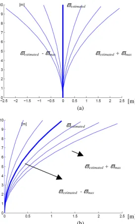
a number of values in the interval [-ϖmax, ϖmax] and then calculating predicted paths for each one give us a set of tracker possible positions for a given time horizon. Assuming that the predicted tracker is centered on the estimated turning rate, ϖestimated (Fig 4), the highest probability value is assigned to the widest path, obtained from ϖestimated. Therefore, the probability decreases as the distance between the predicted paths and the widest one increase.

[m] (a)

[m] (b)

Figure 4. Illustration of Predicted Paths for a tracked obstacle. In (a) the tracker is currently going along the y-axis (ϖϖϖϖestimated) showing 7 possible paths, ranging from left (ϖϖϖϖestimated - ϖϖϖϖmax) to right (ϖϖϖϖestimated + ϖϖϖϖmax) maximum steering angles. In (b) we estimated the current steering angle that allows us to center the predicted paths on it.

Now, based on obstacle class path models, it is possible to implement the predicted occupancy grid map for a given time horizon. Since we decided to represent the robot as a point mass, the occupancy grid had to be enlarged to compensate for the robot sizes (we use the robot circumscribed circumference radius as the occupancy grid growth rate). The predicted occupancy grid map is obtained iteratively for each map update in two steps. In the first step, only the environment static features are considered. They have their occupied cells enlarged by the growth rate, forming a new occupancy grid map with expanded occupied cells (EOC). These cells are considered as having the highest probability of being occupied (probability density equals to 1). Then, from the EOC borders to cell borders that are distant up to the growth rate, the probability densities are linearly decreased reaching zero at the borders. Next, in the final step, the obstacle predicted paths are considered. A number of possible path predictions had been calculated for each tracker and for each path a number of equidistant points are selected along that path. The point selection process takes into account the obstacle class parameters (ϖmax, ϖmin, and maximum acceleration and deceleration) and the desired time horizon. In the sequence, each point is associated with a grid cell

and the process described before for environment static features is applied for all trackers. In the end we obtain an occupancy grid that contains obstacles at present time and their estimated positions at a given time horizon. It is important to emphasize that the predicted occupancy grid map is stored in a separate data structure. It means that the original occupancy grid map is not changed.

One may observe that the predicted occupancy grid map building process may be time and memory consuming depending on the characteristics of the environment. Due to this, we adopted two simplification strategies:

1. We reduced the update frequency for the static part of the occupancy grid map;

2. Obstacles whose distances to the robot are increasing above a threshold value were neglected.

The first strategy is justified because static features usually do not change their positions. But if, for instance, a parked car or a person starts to move unexpectedly, there is always an acceleration period that can be noticed by the obstacle tracking procedure (it immediately reclassifies this obstacle as a mobile one). In spite of this, the new mobile obstacle has its update frequency increased for building the predicted occupancy grid map. Concerning the second strategy, obstacles that are not considered dangerous because they are moving away from the robot are obviously negligible. If they change their path and start to represent a risk, they are not neglected anymore. These two strategies allowed us to keep the time and memory consumptions at an acceptable level during the experiments.

Smart Car Simulator

In the beginning, we developed the algorithms using a MatLab Simulator (Becker et al., 2007-a). It reproduces a simple 2D urban-like environment (approximately 800 m by 800 m) with parked and moving cars, buses, trucks, people, buildings, walls, streets, and trees. When using the simulator, one may reproduce the 2D kinematical behavior of the modified Smart Car. The Smart Car vehicle was kinematically modeled by applying the Ackerman steering geometry (Gillespie, 1992) and the real vehicle dimensions. While modeling the sensors, their real characteristics were taken into account. Lines and/or arcs represent all environment static and dynamic features. The sensor data are extracted from the environment based on its geometrical description and used as input data for testing the algorithms. It is important to emphasize that the simulator also allowed testing the algorithms while the simulated Smart Car was in movement.

Basically, the simulator uses the global position of the Smart Car in the environment for selecting a feature-window that contains all lines and/or arcs close to the vehicle. Then it simulates the laser sensor data by verifying the intersections between the simulated laser beam and the environment features. Afterwards, a noise signal is added to the sensor raw data vector (based on SICK AG, 2006 data). As the simulator was designed for testing different approaches before installing the codes in the real car, it allows the user to select and set different strategies, set points, and threshold values.

Results

Firstly, as cited previously in the text, the research was developed using the Smart Car Simulator. During this phase it was possible to test different techniques for tracking the obstacles. Aiming to facilitate the results comprehension, we present simulations and experimental samples with the vehicle parked in the following figures. Due to this choice, it becomes easier for the reader to compare the features, trackers, etc. at different time spots.

[m] ϖ_estimated

ϖestimated + ϖmax ϖestimated - ϖmax

[m] ϖ_estimated

ϖestimated + ϖmax

(a)

(b)

Figure 5. Simulation of the Smart Car parked in an urban-like environment tracking vehicles on a street cross. Two different time steps are presented. One may observe that vehicles are tracked even when outside the sensor visible area (represented by salmon color). In this case, a pink circle represents the tracker.

Figure 5 shows some simulation results. The trackers inside the range and the matched ones are represented by yellow circles and the hidden or out of range trackers, by pink circles. The black lines represent the obstacle predicted positions for 1 second. All occluded tracks were kept for 1 second. Meanwhile, if they were observed again, their states were updated and they were reclassified as non-hidden tracks. On the other hand, if they were not observed anymore after 1 second, they would be deleted. Regarding the algorithm performance, we compared the moving obstacles estimated speeds with their actual speeds, and the errors observed were less than 5%.

Aiming to test and refine our approach, real sample data were acquired on streets at EPFL. After these tests, it was possible to improve the tracking algorithms. The sites for sampling data were chosen near the parking lots at EPFL for catching as many cars and persons as possible. The sampling took approximately 10 minutes and it was also drawn in the late afternoon when there were people heading home by car. The vehicle was parked in a corner of an intersection where the exit of a parking lot could be seen (Fig. 6-a). We could not use the moving obstacle speeds to verify the algorithm performance because the data sampling took place in a real environment, where we could not control them. However, each tracker had its center point subsequent positions compared with the

estimated ones. Again, the errors were less than 5% (5 Hz data acquisition).

(a)

(b)

Figure 6. Experiment location represented by the x circumscribed in EPFL aerial view and the Sensor Field of View represented by a white transparent area (a) and view of the experimental area (b).

Table 1 – Real data sampling details.

Location EPFL, facing ME G building

Scan Acquisition Frequency 5 Hz

Scan Range 30 m

Scan Angular Resolution 0.5°

Experiment Length 602 seconds

Observed Dynamic Obstacles 33

Table 1 presents some experiment set-up details and the quantity of moving obstacles observed during the data acquisition. We experienced traffic and the obstacles were often passing by close to the sensor. Because of the intersection we were also lucky to capture a few cases when one obstacle occluded another. An interesting condition in this case was that we had many passing bikes. They were sometimes classified as cars, sometimes as pedestrians depending on the viewing angle. Their tire spokes also produced an interesting problem: some of the laser readings acquired by the sensor were behind the bike (the sensor laser beam passed trough the spokes and detected other environment feature that was behind the bike). Due to this, the segmentation algorithm produced erroneous input data for the feature extraction and motion detection algorithms. This problem was solved latter by refining the segmentation algorithm. In the beginning, the segmentation process was based only on consecutive measurements and from then on we decided to also consider the data that are close together, as if belonging to the same object.

When it comes to computer processing power performance, we used a 5 Hz sensor data acquisition frequency. Undoubtedly, the use of a dedicated computer for processing the obstacle tracking task will increase the frequency up to sensor limits (500 KBd data transmission rate for a serial RS422 data interface). We also decided to use a 0.5º angular resolution to detect pedestrians at large distances. The development framework introduced by Fleury et al. (1997) was also used. It allows us to execute the algorithms as Smart Car

Smart Car

Smart Car Position (0,0,0°) Sensor Field

of View

Parking Lot

Out of Range Tracker

Out of Range Tracker Tracker Sensor Field of View

Tracker

0 19 38 57 76 95 [m]

modules on a single laptop running Linux (Dell D505 - Centrino 1.5 GHz). The tasks, coded in GenoM, follow the same approach that is used in embedded systems like typical automotive platforms.

Figures 7 and 8 present more results, now based on real data sampling. In both cases the scanner was placed in the origin (0,0), looking along the positive x-axis and plotted frames which are not consecutive, they were chosen by their contents. On top of each plot, one may observe the time stamp (Time) and the elapsed time between two consecutive scans (dt), both in seconds. The elapsed

time is almost constant, but sometimes, if the sensor detects any error while reading or sending the data, it can take longer because the data is excluded and a new scan data is acquired and sent (compare Fig. 7-g and h). Aiming to facilitate the results comprehension, we present in Fig. 7 only the trackers and in Fig. 8 the predicted occupancy grid.

In Fig. 7 one may observe the trackers (represented by circles), the estimated velocities (represented by line segments), and the static environment features laser sensor readings (represented by dots). The line segments length and direction represent respectively their estimated modulus and direction. In the scenario presented in Fig. 7, two pedestrians were moving towards each other, one from the right and one from the bottom of the scene. A bike was also

traversing, coming from the upper right corner. The trackers continued from (a) to (b) until the moment when the bike went out of range in (c), although the tracker is kept for one second after disappearance. People continued approaching until they were almost perceived as a single segment, (e). In (f), they could be separated again and both trackers were updated. In addition, Fig. 8 shows the trackers, the estimated velocities, the static environment features laser sensor readings, and the predicted occupancy grid map (represented by gray scale cells – as darker the gray cell is as higher is the probability of an cell being occupied). In Fig. 8, the predicted occupancy grid is shown. It is updated at the same scan acquisition frequency (5 Hz). The static environment features were already detected and enlarged by the growth rate, forming the occupancy grid map with EOCs. In (a), a car was coming from the upper right corner and a bike from the bottom. Then the cyclist started to reduce its speed (b) as it approached the intersection. The car kept moving and crossing the intersection until it hid the cyclist (c), but the bike tracker was kept. In (d) the car continued moving and the bike tracker was seen again. The car is not seen anymore in (e) and finally the cyclist turns left in (f).

-20 -10 0 10 20 30 40

-25 -20 -15 -10 -5 0 5 10 15 20 25

X [m] Y

[ m

]

Time: 108.959 [s] dt: 0.207 [s]

-20 -10 0 10 20 30 40

-25 -20 -15 -10 -5 0 5 10 15 20 25

X [m] Y

[ m

]

Time: 113.218 [s] dt: 0.207 [s]

(a) (b)

-20 -10 0 10 20 30 40

-25 -20 -15 -10 -5 0 5 10 15 20 25

X [m] Y

[ m]

Time: 114.493 [s] dt: 0.207 [s]

-20 -10 0 10 20 30 40

-25 -20 -15 -10 -5 0 5 10 15 20 25

X [m] Y

[ m]

Time: 117.276 [s] dt: 0.207 [s]

(c) (d)

Figure 7. Real data sample on streets at EPFL (108.96 s to 120.91 s). Two pedestrians were moving towards each other, one from the right and one from the bottom of the scene. A bike was also traversing, coming from the upper right corner. From (a) to (b) the trackers continued until the moment when the bike went out of range in (c), though the tracker is kept for one second after disappearance. The persons continued approaching until they were almost perceived as a single segment, (e). In (f), they could be separated again and both trackers were updated. The frames are not consecutive.

Pedestrian #1

Pedestrian #2 Bike

Pedestrian #1 Pedestrian #2

Bike

Pedestrian #1 Pedestrian #2

Bike

Pedestrian #1 Pedestrian #2

Out of Range Tracker Smart Car Position

-20 -10 0 10 20 30 40 -25

-20 -15 -10 -5 0 5 10 15 20 25

X [m] Y

[ m

]

Time: 118.334 [s] dt: 0.207 [s]

-20 -10 0 10 20 30 40

-25 -20 -15 -10 -5 0 5 10 15 20 25

X [m] Y

[ m]

Time: 120.911 [s] dt: 0.231 [s]

(e) (f)

Figure 7. (Continued).

(a) (b)

(c) (d)

Figure 8. Real data sample on streets at EPFL (362.26 s to 366.53 s). In (a), a car was coming from the upper right corner and a bike from the bottom. Then, the cyclist started to reduce his speed (b) as he approached the intersection. The car kept moving and crossing the intersection until it hid the cyclist (c), but the bike tracker was kept. In (d) the car continued moving and the bike tracker was seen again. The car is not seen anymore in (e) and finally the cyclist turned left in (f). Observe that the frames are not consecutive.

Pedestrian #2

Pedestrian #1

Car

Bike

Car

Car

Car Bike Bike

Bike Hidden Tracker Smart Car Position

(e) (f)

Figure 8. (Continued).

Conclusions

The successful implementation of car-like mobile robots that are able to move autonomously on streets and roads depends on the vehicle ability of dealing with highly complex environments. Due to this, many researches initially developed for indoor applications are being extended and adapted for outdoor environments. Recently, some algorithms that fuse path planning and obstacle avoidance tasks into a single navigator structure were presented. However, few researches of obstacle path prediction on urban-like environments are being carried out (most of them are centered on vision systems). Our work presented results on obstacle tracking task in dynamic urban-like environments. It focused on 2D laser-based obstacle motion-tracking problem. A Kalman Filter was applied in order to predict the obstacle motions even when they were hidden. First of all, we introduced a short review on the motion tracking techniques found in literature and highlighted the scarcity of publications when it comes to car-like tracking applications in dynamic urban scenarios using laser data. Then, our approach and the test platform used, a modified smart fortwo coupé passenger car named Smart Car, were briefly described. Our approach focused on detection, classification, and tracking tasks of vehicles (e.g.: cars, buses, etc.) and pedestrians. This technique allows the controller to take into account hidden and non-hidden obstacles when maneuvering the vehicle. A probabilistic occupancy-grid representation of the environment, named predicted occupancy grid map, was also implemented. It provided a given time horizon prediction view of the vehicle surroundings based on motion-models of the obstacle classes and obstacle estimated velocities. Real data samples were used to refine the algorithms earlier developed and tested using a MatLab simulator. Finally, the results were presented.

The results using real data samples indicated that obstacle detection, classification, and tracking tasks only with a 2D laser scanner are laborious. It happened because we decided to focus our research on the use of a single sensor in order to obtain a cheaper commercial solution that could be used on passenger cars. Due to this, it was necessary to take into account several environment feature details to turn them into diverse algorithm parameters. For instance, the presence of bushes and leaves can produce spurious readings and induce the algorithm to consider them as moving obstacles. In order to overcome these difficulties, we suggest the use

of road and chart maps of the urban area and GPS, or its differential version (DGPS), combined with embedded cameras. This would increase the system overall performance by promoting data fusion that would allow false mobile obstacles removal and the recognition and classification of obstacles into more detailed classes, e.g.: walls, trees, buses, cars, trucks, bikes, pedestrians, etc. Obviously, as the use of vision systems is computer time expensive and very dependent on scene illumination, it is necessary to work on scene lighting and find a balance between computer processing consumption and adequate data acquisition. Of course, if more computers are used onboard the vehicle, this drawback can be overcome easily. For the moment, this class labeling is carried based only on obstacle speeds and observed sizes. The pedestrian class uses the constant-velocity model and the vehicle class makes use of a simple steering model based on the vehicle ICM for predicting their paths. When it comes to the predicted occupancy grid map building, we adopted two strategies that allowed us to keep the time and memory consumptions at an acceptable level during the experiments: we reduced the update frequency for the static part of the occupancy grid map and we decided to neglect obstacles whose behaviors were not considered dangerous (e.g.: obstacles whose distances to the Smart Car were increasing above a threshold value). Concluding, our results can be considered a valuable step towards promoting the future interface between the motion tracking and dynamic path planning algorithms found in literature. This procedure allows the controller to obtain a better performance in urban-like environments.

Acknowledgments

The first author thanks CAPES for the financial support during his stay at EPFL – ASL (Grant # 0269-05-0), Switzerland. The staffs of EPFL and ETHZ are also due to gratitude for their priceless assistance and remarkable kindness.

References

Bar-Shalom, Y. and Fortmann, T.E., 1998, “Tracking and data association”, Academic Press Inc., London, UK.

Becker, M., Hall, R., Jensen, B., Kolski, S., Maček, K. and Siegwart, R.,

2007-a, “The use of obstacle motion tracking for car-like mobile robots collision avoidance in dynamic urban environments”, Proc. of XII International Symposium on Dynamic Problems of Mechanics – DINAME 2007.

Car

Bike Bike