J. Braz. Soc. Mech. Sci. & Eng. vol.31 número3

!"#$$%&"' () *) + ,

+

+-.$ /&$%'!$ 0 ) +-) + ,

! "

# $

%

&

' " &

%

" ! '

' " (

! '

Turbulent natural convection of air that happens into inner square cavity with localized heating from horizontal bottom surface has been numerically investigated. Localized heating is simulated by a centrally located heat source on the bottom wall, and two values of the dimensionless heat source length ∈ are considered in the present work. Solutions are obtained for several Rayleigh numbers with Prandtl number Pr = 0.70. The horizontal top surface is thermally insulated and the vertical surfaces are assumed to be the cold isothermal surfaces whereas the heat source on the bottom wall is isothermally heated. In this study, the Navier-Stokes equations are used considering a two-dimensional and turbulent flow in unsteady state. The Finite Element Method (FEM) with a Galerkin scheme is utilized for solving the conservation equations. The formulation of conservation equations is carried out for turbulent flow and the implementation of turbulent model is made by Large-Eddy Simulation (LES). The distributions of the stream function and of the temperature are determined as functions of thermal and geometrical parameters. The average Nusselt number Num is shown to increase with an increase in the Rayleigh number Ra as well as in the dimensionless heat source length ∈. The results of this work can be applied to the design of electronic components.

Keywords: cavities, finite element, turbulence, natural convection, LES

Introduction

1_{Natural convection in enclosures is an area of interest due to its}

wide application and great importance in engineering. Transient natural convection flows occur in many technological and industrial applications. Therefore, it is important to understand the heat transfer characteristics of natural convection in an enclosure.

Along the years, researchers have looked for more flows with the objective to approximate the real case found in geophysical or industrial means. Then, we can define four basic types of boundary conditions. They are: the natural convection due to a uniformly heated wall (with a temperature or a constant heat flux); the natural convection induced by a local heat source; the natural convection under multiple heat sources with the same strength and type; and the natural convection conjugated with inner heat-generating conductive body or conductive walls. The boundary conditions mentioned previously are based on a single temperature difference between the differentially heated walls. Most of the previous studies have addressed natural convection in enclosures due to either a horizontally or vertically imposed temperature difference. However, departures from this basic situation are often found in fields such as electronics cooling. The cooling of electronic components is essential for their reliable performance.

The characteristics of fluid flow and heat transfer under the multiple temperature differences are more complicated and have a practical importance in thermal management and design.

In the present work, a two-dimensional numerical simulation in a cavity is carried out for a turbulent flow. The turbulence study is a complex and challenging assumption. There are few works in the literature that deal with natural convection in closed cavities using the turbulence model LES. The motivation to accomplish this work relies on the fact that there is a great number of problems in

Paper accepted December, 2006. Technical Editor: Francisco R. Cunha

engineering that can use this geometry. One turbulence model is implemented here together with the finite element method.

A Large Eddy Simulation (LES) seems as a promising approach for the analysis of the high Grashof number turbulence that contains three-dimensional and unsteady characteristics. A direct simulation of turbulence gives us more accurate and precise data than experiments; it is essentially unsuitable for high Grashof number flows because of computational limitations. It is known that the LES enables an accurate prediction of turbulence, but spends much less CPU time than the direct simulation.

In literature, a large number of theoretical and experimental investigations are reported on natural convection in enclosures.

Natural convection of air in a two-dimensional rectangular enclosure with localized heating from below and symmetrical cooling from the sides was numerically investigated by Aydin and Yang (2000). Localized heating was simulated by a centrally located heat source on the bottom wall, and four different values of the dimensionless heat source length, 1/5, 2/5, 3/5 and 4/5 were considered. Solutions were obtained for Rayleigh number values from 103 to 106. The average Nusselt number at the heated part of the lower wall, Nu, was shown to increase with an increase of the Rayleigh number, Ra, or of the dimensionless heat source length ∈.

Peng and Davidson (2001) studied the turbulent natural convection in a closed enclosure in which vertical lateral walls were maintained at different temperatures. Both the Smagorinsk and the dynamic models were applied to the turbulence simulation. Peng and Davidson (2001) modified the Smagorinsk model by adding the buoyancy term to the turbulent viscosity calculation. This model would be called the Smagorinsk model with buoyancy term. The computed results were compared to experimental data and showed a stable thermal stratification under a low turbulence level (Ra = 1.58 x 109_).

governing equations of natural convection induced by multiple temperature differences. The Rayleigh numbers used were Ra = 103 to 106.

It was performed in the work of Oliveira and Menon (2002) a numerical study of turbulent natural convection in square enclosures. The finite volume method together with LES was used. The enclosure lateral surfaces were kept to different isothermal temperatures, and the upper and lower surfaces were isolated. The flow was studied for low Rayleigh numbers Ra = 1.58 x 109. Three turbulence LES models were used.

Ampofo and Karayiannis (2003) conducted an experimental study of low-level turbulence natural convection in an air filled vertical square cavity. The cavity was 0.75 m high x 1.5 m deep giving rise to a 2D flow. The hot and cold walls of the cavity were isothermal at 50 and 10 ºC respectively, that is, a Rayleigh number equals to 1.58 x 109_{. The experiments that were carried out on}

Ampofo work and Karayiannis (2003) were conducted with very high accuracy and as such the results formed experimental benchmark data and were useful for validation of computational fluid dynamics codes.

Martorell et al. (2003) work dealt with the natural convection flow and heat transfer from a horizontal plate cooled from above. Experiments were carried out for rectangular plates having aspect ratios between φ = 0.036 and 0.43 and Rayleigh numbers in the range of 290 ≤ Raw ≤ 3.3×105. These values of Raw and φ were

selected to the design of printed circuit boards. The results showed that such a low Raw effect could be accounted for in a physically

consistent manner by adding a constant term to the heat transfer correlation.

In the present work, turbulent natural convection of air that happens into inner square cavity with localized heating from horizontal bottom surface has been numerically investigated. The objective of the analyses of heat transfer is to investigate the Nusselt number distribution on the vertical walls and heated lower horizontal surface. Another objective is to verify the effect of height variation I of the horizontal heated lower surface on the turbulent flow. Six cases are studied numerically. The Rayleigh number Ra is varied and so is the dimensionless length the heat source ∈, where (1-∈)/2 ≤x ≤ (1+∈)/2 and x is the coordinate component in the x direction. For the cases 1, 2 and 3, the dimension ∈ is fixed in ∈ = 0.4 and the Rayleigh numbers Ra is varied, in Ra = 107_{, 10}8 _{and 10}9_.

For the cases 1, 2, and 3, it is used a non-structured mesh of finite elements with 5,617 triangle elements and 2,908 nodal points. The other cases also used a non-structured mesh of finite elements with linear triangle elements. In cases 4, 5, and 6, ∈ is fixed in ∈ = 0.8. The cases 1 and 4, 2 and 5, 3 and 6 are simulated, respectively, for Ra = 107, 108 and 109. The cases 4, 5, and 6 are simulated with one mesh with 5,828 elements and 3,015 nodes. The turbulence model used in all cases is the Large-Eddy Simulation (LES) with the second-order structure-function sub-grid scale model (F2). It is

adopted a geometry with an aspect ratio A = H/L = 1.0. Comparisons are made with experimental data and numerical results found in Tian and Karyiannis (2000), Oliveira and Menon (2002), Lankhorst (1991) and Cesini et al. (1999).

Nomenclature

Cθ j = Crossing turbulent flux

di = Distance di from the target point

T

uj = Filtered variable products that describe the turbulent heat transport

j iu

u = Filtered variable products that describe the turbulent momentum transport

Li j = Leonard Tensor

Lθ j = Leonard turbulent flux

Ri j = Reynolds sub-grid tensor

" ij

S = Deformation tensor rater A = Dimensionless constant c = Enclosure aspect ratio

Cij = Crossing tensor

g = Gravity acceleration, m/s2 H = Characteristic dimension of cavity

I = Length of the heated horizontal lower surface L = Characteristic dimension of cavity

ℓ = Scale lengths and the velocity

N = Number of points from the neighborhood n = Unit vector normal to the surface or boundary Nu = Nusselt number

p = Pressure, Pa Pr = Prandtl number q = Velocity, m/s

r = Distance between two points, m Ra = Rayleigh number

S = Source term, Surface T = Temperature, ºC t = Time, s

tCPU = CPU processing times, s

u = Velocity in x direction, m/s v = Velocity in y direction, m/s

x = Coordinate component in x direction y = Coordinate component in y direction

Greek Symbols δij = Kronecker delta

ϕ

= Large eddy component

τij = Reynolds tensor θj = Sub-grid turbulent flux

νT = Turbulent kinematic viscosity

ε = Dissipation of the turbulent kinetic energy ε

φ = Aspect ratio

∈ = Dimensionless heat source length

Ω = Studied domain

ρ = Fluid density

β = Fluid volumetric expansion coefficient

ϕ = General variable

∆ = Geometric mean of distances di from neighboring

elements to the point where vT is calculated ∆1 = Filter length in x direction

∆2 = Filter length in y direction ν = Kinematic viscosity

ψ = Stream function

α = Thermal diffusivity

ω = Vorticity

Subscripts

m relative to mean

i relative to i directions

j relative to j directions

k relative to k directions

T relative to turbulent

c relative to cold

h relative to hot

w Wall

Problem Description and Hypothesis

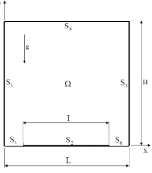
Figure 1 shows the geometry with the domain . It will be considered a square cavity. The upper horizontal surface S4 is

thermally insulated and the vertical surfaces S1 and S3 are assumed

to be the cold isothermal surfaces. The bottom horizontal surfaces S5

and S6 are also thermally insulated. Localized heating is simulated

by a centrally located heat source on the bottom wall, S2. The initial

condition in is: T = 0 with ψ = ω = 0. All physical properties of the fluid are constant except the density in the buoyancy term, where it obeys the Boussinesq approximation. It is assumed that the third dimension of the cavities is large enough so that the flow and heat transfer are two-dimensional.

Figure 1. Cavity geometry

Theory of Sub-Grid Scale Modelling

The governing conservation equations are:

0 = ∂ ∂ i i x u (1)

(

)

ij i j j i j i j j i

i _{g T T}

x u x u v x x p x u u t u δ β ρ 0 1 − +                 ∂ ∂ + ∂ ∂ ∂ ∂ + ∂ ∂ − = ∂ ∂ + ∂ ∂ (2) S +         ∂ ∂ ∂ ∂ = ∂ ∂ + ∂ ∂ j j j j x T x x T u t

T _α (3)

where xi are the axial coordinates x and y, ui are the velocity

components, p is the pressure, T is the temperature, ρ is the fluid density, νis the kinematic viscosity, g is the gravity acceleration, β is the fluid volumetric expansion coefficient, δijis the Kronecker delta, α is the thermal diffusivity, and S the source term. The last term in Eq. (2) is the Boussinesq buoyancy term where T0 is the

reference temperature.

In the Large Eddy Simulation (LES), a variable decomposition similar to the one in the Reynolds decomposition is performed, where the quantity ϕ is split as follows:

'

ϕ ϕ

ϕ= + (4)

where

ϕ

is the large eddy component and ϕ' _{is the small eddy} component.

Figure 2 shows one of the meshes used in the numerical simulations of the present work.

Figure 2. Mesh arrangement for cases 1, 2 and 3.

The following hypotheses are employed in the present work: unsteady turbulent regime; incompressible two-dimensional flow; constant fluid physical properties, except the density in the buoyancy terms.

The following filtered conservation equations are shown after applying the filtering operation to Eqs. (1) to (3). It is done by using the volume filter function presented in Krajnovic (1998). The density is constant.

0 = ∂ ∂ i i x u (5)

(

)

j

i j j i j i j j i

i _{g T T}

x u x u v x x p x u u t u 2 0

1 _{β δ}

ρ _+ −

               ∂ ∂ + ∂ ∂ ∂ ∂ + ∂ ∂ − = ∂ ∂ + ∂ ∂ (6) S +         ∂ ∂ ∂ ∂ = ∂ ∂ + ∂ ∂ j j j j x T x x T u t T α (7)

In the Eqs. (5) to (7), j iu

u and _uT

According to Oliveira and Menon (2002), the products j iu u and

T

uj are split into other terms by including the Leonard tensor Lij, the Crossing tensor Cij, the Reynolds sub-grid tensor Rij, the

Leonard turbulent flux L_θj, the Crossing turbulent flux Cθ j and the

sub-grid turbulent flux θj. The Crossing and Leonard terms, according to Padilla (2000), can be neglected. After the development shown in Oliveira and Menon (2002), the following conservation equations are obtained:

0 = ∂ ∂ i i x u (8)

(

)

ij i ij j j i i j j i

i _{g T T}

x x x u x p x u u t

u _ν τ _{β δ}

ρ 0

2

1 _{+ −}

∂ ∂ −         ∂ ∂ ∂ + ∂ ∂ − = ∂ ∂ + ∂ ∂ (9) j j j j j j x x T x x T u t T ∂ ∂ +         ∂ ∂ ∂ ∂ = ∂ ∂ + ∂

∂ _α θ (10)

where Pr is the Prandtl number with α = ν / Pr. The tensors τij and

θj that appear in Eqs. (9) and (10) are modeled in the forthcoming topics.

Sub-grid scale model

Many sub-grid scale models use the diffusion gradient hypothesis similar to the Boussinesq one that expresses the subgrid Reynolds tensor in function of the deformation rate and kinematic energy. According to Silveira-Neto (1998), the Reynolds tensor is defined as:

kk ij ij T

ij ν S δ S

τ 3 2 2 − − = (11)

where vT is the turbulent kinematic viscosity, δij is the Kronecker

delta, and Sij is deformation tensor rate given by:

i j j i ij x u x u S ∂ ∂ + ∂ ∂ = (12) Substituting ij

S , from Eq. (12), in Eq. (11) and manipulating equations, we have:

(

)

ij

i j j i T j j j i i j j i i T T g x u x u x x x u x p x u u t u δ β ν ν ρ 0 2 1 − +                 ∂ ∂ + ∂ ∂ ∂ ∂ +         ∂ ∂ ∂ + ∂ ∂ − = ∂ ∂ + ∂ ∂ (13)

In a similar way, the energy equation is obtained:

(

)

        ∂ ∂ + ∂ ∂ = ∂ ∂ + ∂ ∂ j T j j j x T x x T u t

T _{α α} (14)

where the turbulent thermal diffusivity αT is calculated as:

αT = νT / PrT (15)

and PrT is the turbulent Prandtl number.

The sub-grid models give the following expression for the turbulent viscosity vT:

q c

T =

ν

(16)

where c is a dimensionless constant, and q are the scale lengths and the velocity, respectively.

The parameter is related to the filter size and it is usually used in the two-dimensional case with a rectangular element as:

ℓ = _

∆

= (∆1∆2)1/2 (17)

where 1 and 2 are the filter lengths in x and y directions.

The second-order structure-function sub-grid scale model (F2)

The turbulent viscosity vT is calculated as follows:

(

x t

)

C F

(

x t

)

vT ,∆, =0.104 k−3/2∆ 2 ,∆, (18)

where Ck = 1.4 is the Kolmogorov constant (Kolmogorov, 1941).

The variable is the geometric mean of distances di from

neighboring elements to the point where vT is calculated and is given

by:

N i N

i=1

d

Π

=

∆

(19)

and F2

(

x,∆,t

)

is the structure function of second order velocities.

According to Kolmogorov (1941) law that establishes that the structure function of second order velocities is proportional to (εr)2/3, where r is the distance between two points, the structure function can be calculated as:

(

) ( )

[

]

{{

(

)

[

]

}

         _∆ − + + + − + Σ = = 3 / 2 2 2 1 2 ) , ( , , , 1 i i i i i i i N i d t x t e d x t x u t e d x u N F υ υ (20)

where u_i

(

x+d_ie_i,t

)

and

υ

_i

(

x+d_ie_i,t

)

are the velocities at the point “i” of the neighboring centroid placed at a distance di from the target point, u(x,t)and

υ

(x,t) are the velocities at this point of the element, N is the number of points from the neighborhood, t is the time and e_ithe vector on i direction.

The turbulent thermal diffusion is estimated from the turbulent kinematic viscosity, by assuming:

Initial and boundary conditions

From this section on, the upper bars that mean average values will be omitted.

Figure 1 pictures the enclosure on which the initial boundary conditions are as follows:

(

x,y,0)

)

=0, v

(

x,y,0)

)

=0, T

(

x,y,0)

)

=0

u (22)

0 ,

0 = =

=

=v T Tc

u (23)

1 ,

0 = =

=

=v T Th

u (24)

0 / ,

0 ∂ ∂ =

=

=v T y

u (25)

The flow field can be described by the stream function ψ and the vorticity ω distributions given by:

(

x

) (

u y

)

x y

u=∂

ψ

/∂ ,

υ

=−∂

ψ

/∂ ,

ω

= ∂

υ

/∂ − ∂ /∂ (26) where u and ν are the velocity components in x and y directions, respectively. Hence, the continuity equation given by Eq. (1) is exactly satisfied. Working with dimensionless variables, it is possible to deal with Rayleigh number Ra, Prandtl number Pr and the enclosure aspect ratio A given by:

(

)

[

3 2

]

7 8 9

10 10 , 10 /

Prg T T H v and

Ra= β h− c = ,

Pr = ν /α = 0.7,

A = H/L = 1.0 (27)

where Th and Tc are the temperatures on surfaces S2 and S1 - S3,

respectively. H is the characteristic dimension of cavity.

Numerical method

Equations (8) to (10) are solved through the finite element method (FEM) with linear triangular elements using the Galerkin formulation. The system of equations is solved with the Gauss

Quadrature. The problem solution follows the steps below: (1) through Eq. (26), the stream function field ψ is solved; (2) the wall vorticity is determined in matricial form, according to Silveira-Neto et al. (2000); (3) the boundary conditions for vorticity are applied; (4) the vorticity in the interior is calculated according to Eq. (26); (5) the temperature field is solved through Eq. (10); (6) the local Nusselt number Nu is obtained using Eq. (28); (7) the time is increased with the time step ∆t and the iteration with unity, and then it turns to the first step (1). It starts all over again till it reaches the stop criterion.

The local Nusselt number Nu is defined as:

(

T n

)

wH

(

Th Tc

)

Nu= ∂ ∂ − (28)

where n is the unit vector normal to the surface or boundary, where the local Nusselt number Nu is calculated.

Numerical method validation

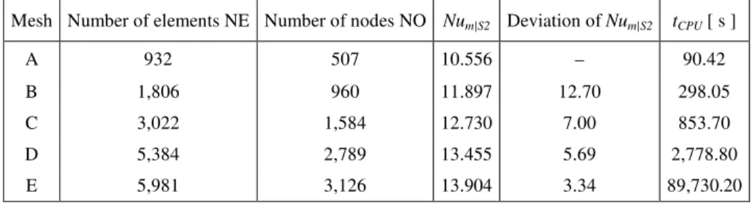
In the present work, a study of the effect of mesh refinement on the average Nusselt number Num calculated on hot lower surface S2 is conducted. The thermal parameters used are: Rayleigh number Ra = 106 and Prandtl number Pr = 0.71. The geometric parameters used are: cavity aspect ratio A = 1.0 and dimensionless length of heated source ∈ = 0.5. Five mesh types are used. Table 1 shows the results obtained in this mesh study. After this study, we adopted a computational mesh between meshes D and E.

In order to compare the results with the ones found in literature and then to validate the computational code in FORTRAN, two cases are taken from Brito et al. (2002) and Brito et al. (2003). Brito et al. (2002) and Brito et al. (2003) use the same turbulence model LES as the one used in the present work. In the first comparison, the study of the natural turbulent flow in a square enclosure with different temperatures for various Rayleigh numbers is carried out in Brito et al. (2002). The second comparison is made in Brito et al. (2003) considering a laminar flow in a rectangular enclosure with an internal cylinder.

Table 1. Numeric results obtained by Nusselt Num in the heated lower surface S2.

Mesh Number of elements NE Number of nodes NO Num|S2 Deviation of Num|S2 tCPU [ s ]

A 932 507 10.556 – 90.42

B 1,806 960 11.897 12.70 298.05

C 3,022 1,584 12.730 7.00 853.70

D 5,384 2,789 13.455 5.69 2,778.80

E 5,981 3,126 13.904 3.34 89,730.20

In the first comparison, it is also used the Large Eddy Simulation (LES). The results in Brito et al. (2002) are compared not only to the experimental and numerical ones in Peng and Davidson (2001), and Tian and Karayiannis (2000), but also to the numerical ones in Lankhorst (1991). In the comparisons realized in Brito et al. (2002), measures for the center of square cavity for dimensionless average velocity are made. The results showed good concordance with the experimental results.

hand, the cylinder surface has a high temperature Th. In the second comparison, the maximum deviation is 11.88 % with Rayleigh number equals to 3.4 x 103 using a mesh with 5,790 elements and 3,011 node points. The minor deviation is 7.53 % to Rayleigh number equals to 3.0 x 104.

Results

The main objective of this study is to analyze the influence of Rayleigh number’s variation and the length I of the heated horizontal lower surface on the flow field. The geometry is chosen in order to simulate the cooling of the air in cavities with electronic components placed on the lower horizontal surface. A range of Rayleigh numbers in a low turbulence flow is used. The thermal parameters used are: Ra = 1.0 x 107, 1.0 x 108, and 1.0 x 109 with Pr = 0.70. The geometry parameters used in the six cases mentioned previously are: H = 1.0; L = 1.0; Th = 1; Tc = 0 and A = H / L = 1.0. In order to model the turbulence, it is used the Large-Eddy Simulation (LES) with the second-order structure-function sub-grid scale model (F2). In this work, we also make a study of effect of the mesh refinement, aiming to obtain the best time computational cost. It is used a program in FORTRAN, with the Compaq Visual Fortran v6.6 compilator, for the realization of the numeric simulation. The numeric results are obtained using one Intel Pentium III processor of 800 MHz with 128 MB memory RAM (see Table 1 for CPU processing times tCPU in seconds).

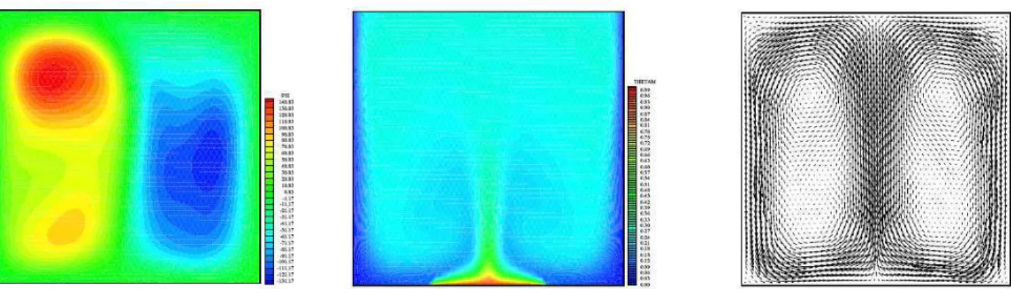
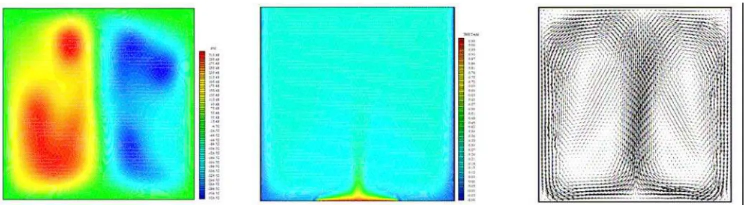
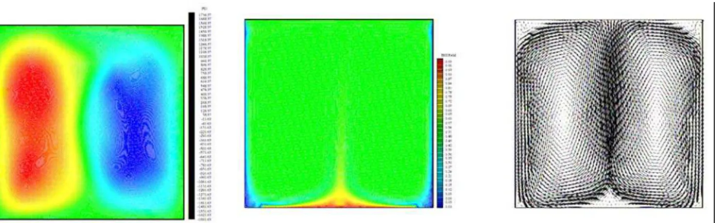
Figures 3 and 4 present the local Nusselt number Nu versus the coordinate x for horizontal lower surfaces S2, S5 and S6. Figures 5-10 show the average Nusselt number Num versus time for all six cases. Figures 11-16 show the flow fields and the temperature in terms of stream function lines ψ, isotherms Tm and velocity vectors ui. The time step ∆t adopted in this present work is based on Peng and Davidson work (2001), where ∆t = 0.0131 t0, t0 = H / (g β∆t H)1/2. In the present work, due to the limitation of the hardware (processor), we adopt one time step ∆t three times bigger than the value adopted in Peng and Davidson work (2001). In Figures 5-10, the average time to obtain the average quantities is from 400 to 600t0, t = (400 - 600) t0. Figures 11-16 show the stream function ψ with a line spacing equals to 10 (∆ψ = 10). For the isotherms, we adopt the same line spacing in all Figs. 11-16, ∆tm = 0.01. The stream function ψ is shown for the last interaction, t = 600t0. The isotherms are calculated at each nodal point considering an average time, that is, t = (400-600) t0. The same was done to the velocity vectors ui.

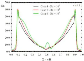
Figures 3 and 4 show the distribution of local Nusselt number Nu along all the lower horizontal surface S2. Figures 3 and 4 show the results for heated lengths ∈ = 0.4 and 0.8, for the last time (t = 600t0). We observe that increasing ∈, Nu increases in the horizontal lower heated surface. For a fixed value of ∈, Ra increase does not result in a heat exchange on surface S2. We also observe a certain symmetry of the heat transfer in the middle of the cavity (x = L/2), even for higher Ra (Ra = 109).

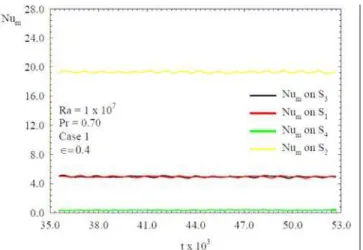
Figures 5-10 show the average Nusselt numbers Num calculated on surfaces S1, S2, S3 and S4, versus time t for a time range t = (400 - 600) t0. Figures 5, 6, and 7, show that the higher the Rayleigh number, the higher the convection in all cavity surfaces studied for fixed values of ∈. Figures 8, 9 and 10 show that heat transfer is higher when the Rayleigh number is increased. In Fig. 10, the Num values oscillate, due to the effect of the turbulence inside the cavity. The rates of heat transfer are a little larger than those presented in Figs. 5, 6, and 7. In Figures 5 to 10, where Ra = 107, the ∈ increase does not considerably influence

the values of Num. Figures 6 and 9, for Ra = 108, show that the ∈ increase reduces Num on S2. In Figs. 7 and 10, for Ra = 109, we observe the same behavior found in Figs. 6 and 9 with Ra = 108. Then, we can conclude that the flow become oscillating for Ra = 108 and ∈ = 0.8, and, as it can be seen in Fig. 10, the heat transfer rates are larger on all the surfaces, including the upper horizontal surface S4.

Figure 3. Local Nusselt number Nu on S2, S5 and S6 surfaces for R = 107, 108 e 109 with t = 600 t0 for cases 1, 2 and 3 (∈∈∈∈ = 0.4).

Figure 5. Num versus t on S1, S2, S3 and S4 with Pr = 0.70, ∈∈∈∈ = 0.4 and

t = (400-600) t0, for R = 107.

Figure 6. Num versus t on S1, S2, S3 and S4 with Pr = 0.70, ∈∈∈∈ = 0.4 and

t = (400-600) t0, for R = 108.

Figure 7. Num versus t on S1, S2, S3 and S4 with Pr = 0.70, ∈∈∈∈ = 0.4 and

t = (400-600) t0, for R = 109.

Figure 8. Num versus t on S1, S2, S3 and S4 with Pr = 0.70, ∈∈∈∈ = 0.8 and

t = (400-600) t0, for R = 107.

Figure 9. Num versus t on S1, S2, S3 and S4 with Pr = 0.70, ∈∈∈∈ = 0.8 and

t = (400-600) t0, for R = 108.

Figure 10. Num versus t on S1, S2, S3 and S4 with Pr = 0.70, ∈∈∈∈ = 0.8 and

Figures 11-16 show the effect of Rayleigh number, where 107≤ Ra ≤ 109, and the effect of the dimensionless length of heat source for ∈ = 0.4 and 0.8. Due to the symmetrical boundary conditions along the vertical walls, the flow and the temperature fields have a relative symmetry in the middle of the cavity. For the temperature field, we observe that this symmetry is better visualized, because the isotherms are obtained through an average in the time for t = (400 - 600) t0. These same symmetrical boundary conditions in the vertical direction result in two great fluid areas that symmetrically recirculate. As the flow tends to the oscillating regime for Ra = 109, this symmetry is lost.

In Figs. 11, 12 and 13, where ∈ = 0.4, it is observed that the internal fluid recirculation is more significant as Ra increases. For Ra ≤ 107, thermal plumes are formed over the hot surface S2. The hot fluid, which is in the lower region of the cavity, moves up due to buoyant forces. During its traveling to the upper part of the cavity, the fluid is cooled in vertical lateral walls. It can be noted in Fig. 12 that with the Ra increase to Ra ≤ 108_{, a region with lower heat}

transfer is brought about giving rise to a smaller thermal plume. In Fig. 13, for Ra ≤ 109_{, practically all the fluid inside the cavity has a}

stable average temperature between the maximum and minimum values stated by the boundary conditions. From Figs. 11, 12 and 13, the average velocity vectors picture the fluid behavior in the time range t = (400 - 600) t0.

Figures 14, 15, and 16 show the results for ∈ = 0.8 and Ra between 107 ≤ Ra ≤ 109. For Figs. 14, 15 and 16, where ∈ = 0.8, the increase of the heated surface length S2 makes the heat transfer increase in all surfaces, as seen in the graphics of Num versus the time t. The surface S2 has the reduction of the Num value calculated for the range 400 to 600 t0 with Ra = 107. For the isotherms, Figs. 15 and 16 show few differences. The streamlines in Figures 14, 15 and 16 show two big fluid regions that recircle in opposite directions.

Discussion

In this investigation, the results of a numerical study of buoyancy-induced flow and heat transfer in a two-dimensional square enclosure with localized heating from below and symmetrical cooling from the sides are presented. The main parameters of interest are Rayleigh number Ra and the dimensionless heat source length ∈.

One kind of sub-grid scale model is used: large-eddy simulation (LES) with the second-order structure-function subgrid scale model (F2) (more details in Silveira-Neto, 1998). The conservation equations are discretized by the Galerkin finite element method with linear triangular elements.

Two cases are used for validation of the computational domain of the present work. As in Brito et al. (2002) and Brito et al. (2003), the same turbulence model LES together with the finite element method is used in the present work.

It is observed that increasing Ra, the rate of heat transfer also increases, as expected. For a fixed value of Ra, the ∈ increase also increases the heat transfer. For Ra = 109 and ∈ = 0.8, although the flow is considered two-dimensional, it is noticed that the flow becomes oscillating in time, which is a typical characteristic of a flow in transition to turbulence.

The average temperature Tm and velocity vectors ui distributions are presented for Rayleigh number 107 ≤ _Ra ≤ ₁₀9 _{and Prandtl}

number Pr = 0.70 for t = (400 - 600) t0. The results of stream function ψ distributions are presented for t = 600 t0.

Acknowledgements

The authors thank the financial support from CNPq and CAPES without which this work would be impossible.

Figure 11. Case 1 – Streamfunction ψψψψ for t = 600 t0 (∆∆∆∆ψψψψ = 10), average temperature Tm (∆∆∆∆Tm = 0.01) for t = (400-600) t0,and velocity vectors for

Figure 12. Case 2 – Streamfunction ψψψψ for t = 600 t0 (∆∆∆∆ψψψψ = 10), average temperature Tm (∆∆∆∆Tm = 0.01) for t = (400-600) t0,and velocity vectors for

t = (400-600) t0– R = 108– Pr = 0.7 – ∈∈∈∈= 0.4.

Figure 13. Case 3 – Streamfunction ψψψψ for t = 600 t0 (∆∆∆∆ψψψψ = 10), average temperature Tm (∆∆∆∆Tm = 0.01) for t = (400-600) t0, and velocity vectors for

t = (400-600) t0– R = 109– Pr = 0.7 – ∈∈∈∈ = 0.4.

Figure 14. Case 4 – Streamfunction ψψψψ for t = 600 t0 (∆∆∆∆ψψψψ = 10), average temperature Tm (∆∆∆∆Tm = 0.01) for t = (400-600) t0,and velocity vectors for

Figure 15. Case 5 – Streamfunction ψψψψ for t = 600 t0 (∆∆∆∆ψψψψ = 10), average temperature Tm (∆∆∆∆Tm = 0.01) for t = (400-600) t0,and velocity vectors for

t = (400-600) t0– R = 108– Pr = 0.7 – ∈∈∈∈ = 0.8.

Figure 16. Case 6 – Streamfunction ψψψψ for t = 600 t0 (∆∆∆∆ψψψψ = 10), average temperature Tm (∆∆∆∆Tm = 0.01) for t = (400-600) t0,and velocity vectors for

t = (400-600) t0– R = 109– Pr = 0.7 – ∈∈∈∈ = 0.8.

References

Ampofo, F. and Karayiannis, T.G., 2003, “Experimental benchmark data for turbulent natural convection in an air filled square cavity”, International Journal of Heat and Mass Transfer, Vol. 46, pp 3551–3572.

Aydin, O. and Yang, W.-J., 2000, “Natural convection in enclosures with localized heating from below and symmetrical cooling from sides”,

International Journal of Numerical Methods for Heat & Fluid Flow, Vol. 10, No. 5, pp 518-529.

Brito, R. F., Guimarães, P. M., Silveira-Neto, A., Oliveira, M. and Menon, G. J., 2003, “Turbulent natural convection in a rectangular enclosure using large eddy simulation”, Proceedings of the COBEM 17th _{International}

Congress of Mechanical Engineering, São Paulo, Brazil, pp 1-10.

Brito, R. F., Silveira-Neto, A., Oliveira, M. and Menon, G. J., 2002, “Convecção natural turbulenta em cavidade retangular com um cilindro interno”, Proceedings of the MECOM 1st _{South-American Congress on}

Computational Mechanics, and III Brazilian Congress on Computational Mechanics, and VII Argentine Congress on Computational Mechanics, Santa Fe, Argentina, pp 620-633. (In Portuguese)

Cesini, G., Paroncini, M., Cortella G. and Manzan, M., 1999, “Natural convection from a horizontal cylinder in a rectangular cavity”, International Journal of Heat and Mass Transfer, Vol. 42, pp 1801-1811.

Deng, Q.-H., Tang, G.-F. and Li, Y., 2002, “A combined temperature scale for analyzing natural convection in rectangular enclosures with discrete wall heat sources”, International Journal of Heat and Mass Transfer, Vol. 45, pp 3437–3446.

Kolmogorov, A. N., 1941, “The local structure of turbulence in incompressible viscous fluid for very large Reynolds numbers”, Dokl. Akad. Nauk SSSR, Vol. 30, No.4, pp. 301-305, and also in: Proceedings of Royal Society of London, 1991, Vol. 434, pp. 9-13.

Krajnovic, S., 1998, “Large-Eddy Simulation of the Flow Around a Surface Mounted Single Cube in a Channel”, M.Sc. Thesis, Chalmers University of Technology, Goteborg, Sweden.

Lankhorst, A. M., 1991, “Laminar and Turbulent Natural Convection in Cavities – Numerical Modelling and Experimental Validation”, Ph.D. Thesis, Technology University of Delft, The Netherlands.

Oliveira, M. and Menon, G. J., 2002, “Simulação de grandes escalas utilizada para convecção natural turbulenta em cavidades”, Proceedings of the ENCIT 9th _{Congresso Brasileiro de Engenharia e Ciências Térmicas ,}

Caxambu, Brazil, CD ROM, pp 1-11. (In Portuguese)

Padilla, E. L. M., 2000, “Simulação Numérica de Grandes Escalas com Modelagem Dinâmica, Aplicada à Convecção Mista”, M.Sc. Thesis, Federal University of Uberlandia, Uberlândia, Brazil. (In Portuguese)

Peng, S. H. and Davidson, L., 2001, “Large-eddy simulation for turbulent buoyant flow in a confined cavity”, International Journal of Heat and Fluid Flow, Vol. 22, pp 323-331.

Silveira-Neto, A., 1998, “Simulação de grandes escalas de escoamentos turbulentos”, In: I ETT Escola de Primavera de Transição e Turbulência, Vol.1, Rio de Janeiro, Brazil, pp 157-190. (In Portuguese)

Silveira-Neto, A., Brito, R. F., Dias, J. B. and Menon, G. J., 2000, “Aplicação da simulação de grandes escalas no método de elementos finitos para modelar escoamentos turbulentos”, In: II ETT Escola Brasileira de Primavera, Transição e Turbulência, Uberlândia, Brazil, pp 515-526. (In Portuguese)

Tian, Y. S. and Karayiannis, T. G., 2000a, “Low turbulence natural convection in an air filled square cavity – part I: the thermal and fluid flow fields”, International Journal of Heat and Mass Transfer, Vol. 43, pp 849-866. Tian, Y. S. and Karayiannis, T. G., 2000b, “Low turbulence natural convection in an air filled square cavity - part II: the turbulence quantities”,